© B.J. Korites 2018
B.J. KoritesPython Graphicshttps://doi.org/10.1007/978-1-4842-3378-8_5

5. Intersections

B. J. Korites1 
(1)
Duxbury, Massachusetts, USA
 

In this chapter, you will develop algorithms that will tell you where lines and planes intersect a variety of objects. The techniques you develop will be useful later when you remove hidden lines and trace shadows cast by objects. You will also learn how to show the intersection of lines and planes with a sphere. As you will see, there is no one magic algorithm that will satisfy all situations; each requires its own methodology. While you may never need some of these algorithms, such as a line intersecting a circular sector, the procedures, which rely on vector-based geometry, are interesting and should give you the tools you will need when you encounter different situations.

Instead of using vectors, many of these solutions could be derived analytically. For example, the solution for a line intersecting a sphere can be obtained by combining the equation of a line with that of a sphere. The result is a quadratic equation that, when solved, yields the entrance and exit points. Such an approach can be fast and simple provided you are dealing with objects that can be represented by simple equations. However, the vector-based procedures, while they may seem more complex, are actually quite simple and intuitive. They can also be much more versatile and adaptable to unusual situations. They are the ones you will use here.

5.1 Line Intersecting a Rectangular Plane

Figure 5-1 shows a line intersecting a rectangular plane . You will develop the algorithm and a program to find the point of intersection, called the hit point. Here you are stipulating that the plane is finite, but it doesn’t have to be. After going through the analysis, you will see there is nothing here that requires the plane be finite. You also start off by assuming the plane is rectangular. It doesn’t have to be rectangular but, for now, it is easier to keep it finite and rectangular.
../images/456962_1_En_5_Chapter/456962_1_En_5_Fig1_HTML.jpg
Figure 5-1

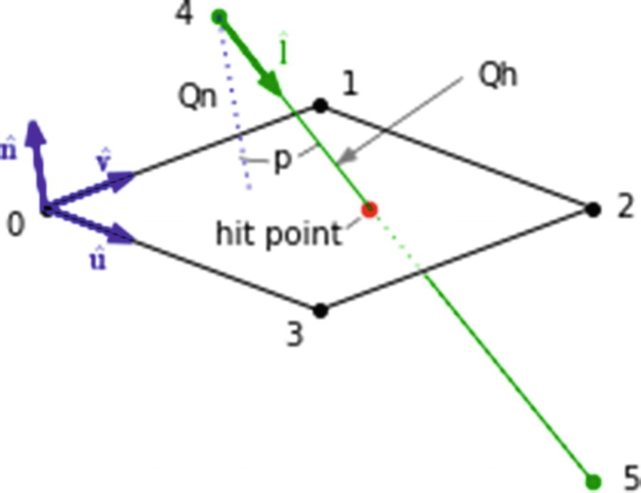
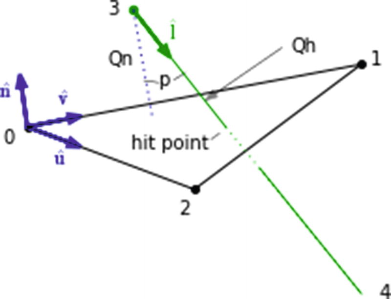
Geometry of a line intersecting a rectangular plane

The plane has corners at 0, 1, 2, and 3. These have local coordinates of (x0,y0,z0) - (x3,y3,z3) relative to the center of rotation at (xc,yc,zc). The line starts at x[4],y[4],z[4] and ends at x[5],y[5],z[5]. It intersects the plane at the hit point.

There are three unit vectors at corner 0; û,$$ widehat{mathbf{v}} $$, and $$ widehat{mathbf{n}} $$. Unit vector $$ widehat{mathbf{v}} $$ points from corner 0 to 1; û from 0 to 3. $$ widehat{mathbf{n}} $$ is normal to the plane. $$ widehat{mathbf{l}} $$ is a unit vector pointing along the line from 4 to 5. Q45 is the distance from 4 to 5. Q h is the distance from 4 to the hit point. Q n is the perpendicular distance from 4 to the plane. Your quest is to determine the location of the hit point (xh,yh,zh). Using vector geometry, you can write the following relations:

Distance 4 → 5:
$$ a=xleft[5
ight]-xleft[4
ight] $$
(5-1)
$$ b=yleft[5
ight]-yleft[4
ight] $$
(5-2)
$$ c=zleft[5
ight]-zleft[4
ight] $$
(5-3)
$$ {Q}_{45}=sqrt{a^2+{b}^2+{c}^2} $$
(5-4)
Unit vector 4 → 5:
$$ lx=frac{a}{Q_{45}} $$
(5-5)
$$ ly=frac{b}{Q_{45}} $$
(5-6)
$$ lz=frac{c}{Q_{45}} $$
(5-7)
$$ widehat{mathbf{I}}= lxwidehat{mathbf{i}}+ lywidehat{mathbf{j}}+ lzwidehat{mathbf{k}} $$
(5-8)
Distance 0 → 3:
$$ a=xleft[3
ight]-xleft[0
ight] $$
(5-9)
$$ b=yleft[3
ight]-yleft[0
ight] $$
(5-10)
$$ c=zleft[3
ight]-zleft[0
ight] $$
(5-11)
$$ {Q}_{03}=sqrt{a^2+{b}^2+{c}^2} $$
(5-12)
Unit vector 0 → 3:
$$ ux=frac{a}{Q_{03}} $$
(5-13)
$$ uy=frac{b}{Q_{03}} $$
(5-14)
$$ uz=frac{c}{Q_{03}} $$
(5-15)
$$ widehat{mathbf{u}}= uxwidehat{mathbf{i}}+ uywidehat{mathbf{j}}+ uzwidehat{mathbf{k}} $$
(5-16)
Distance 0 → 1:
$$ a=xleft[1
ight]-xleft[0
ight] $$
(5-17)
$$ b=yleft[1
ight]-yleft[0
ight] $$
(5-18)
$$ c=zleft[1
ight]-zleft[0
ight] $$
(5-19)
$$ {Q}_{01}=sqrt{a^2+{b}^2+{c}^2} $$
(5-20)
Unit vector 0 → 1:
$$ vx=frac{a}{Q_{01}} $$
(5-21)
$$ vy=frac{b}{Q_{01}} $$
(5-22)
$$ vz=frac{c}{Q_{01}} $$
(5-23)
$$ widehat{mathbf{v}}= vxwidehat{mathbf{i}}+ vywidehat{mathbf{j}}+ vzwidehat{mathbf{k}} $$
(5-24)
Unit vector $$ widehat{mathbf{n}} $$:
$$ widehat{mathbf{n}}=widehat{mathbf{u}}	imes widehat{mathbf{v}} $$
(5-25)
$$ =left[egin{array}{ccc}widehat{mathbf{i}}& widehat{mathbf{j}}& widehat{mathbf{k}}\ {} ux& uy& uz\ {} vx& vy& vzend{array}
ight] $$
(5-26)
$$ widehat{mathrm{n}}=widehat{mathbf{i}}underset{nx}{underbrace{left( uycdotp vz- uzcdotp vy
ight)}}+widehat{mathbf{j}}underset{ny}{underbrace{left( uzcdotp vx- uxcdotp vz
ight)}}+widehat{mathbf{k}}underset{nz}{underbrace{left( uxcdotp vy- uycdotp vx
ight)}} $$
(5-27)
$$ widehat{mathbf{n}}= nxwidehat{mathbf{i}}+ nywidehat{mathbf{j}}+ nzwidehat{mathbf{k}} $$
(5-28)
$$ nx= uycdotp vz- uzcdotp vy $$
(5-29)
$$ ny= uzcdotp vx- uxcdotp vz $$
(5-30)
$$ nz= uxcdotp vy- uycdotp vx $$
(5-31)
Vector 0 → 4:
$$ {mathbf{V}}_{04}=v{x}_{04}widehat{mathbf{i}}+v{y}_{04}widehat{mathbf{j}}+v{z}_{04}widehat{mathbf{k}} $$
(5-32)
$$ v{x}_{04}=xleft[4
ight]-xleft[0
ight] $$
(5-33)
$$ v{y}_{04}=yleft[4
ight]-yleft[0
ight] $$
(5-34)
$$ v{z}_{04}=zleft[4
ight]-zleft[0
ight] $$
(5-35)
Perpendicular distance 4 to plane:
$$ {Q}_n=left|{mathbf{V}}_{04}cdotp widehat{mathbf{n}}
ight| $$
(5-36)
Hit point:
$$ {Q}_n={Q}_hkern0.1em mathit{cos}(p) $$
(5-37)
$$ {Q}_h=frac{Q_n}{mathit{cos}(p)} $$
(5-38)
$$ mathit{cos}(p)=widehat{mathbf{l}}cdotp widehat{mathbf{n}} $$
(5-39)
$$ = lxcdotp nx+ lycdotp ny+ lzcdotp nz $$
(5-40)
$$ xh=xleft[4
ight]+{Q}_h lx $$
(5-41)
$$ yh=yleft[4
ight]+{Q}_h ly $$
(5-42)
$$ zh=zleft[4
ight]+{Q}_h lz $$
(5-43)

You can test to see if the hit point lies within the boundaries of the plane. Figure 5-2 shows the geometry. Vector V0h runs from corner 0 to the hit point h. up and vp are the projections of V0h on the 03 and 01 directions, respectively. To test for an in-bound or out-of-bound hit,

if up < 0 or up > Q03    hit is out of bounds

if vp < 0 or vp > Q01     hit is out of bounds

With xh,yh, and zh being the coordinates of the hit point h, you can calculate up and vp as follows:
$$ a= xh-xleft[0
ight] $$
(5-44)
$$ b= yh-yleft[0
ight] $$
(5-45)
$$ c= zh-zleft[0
ight] $$
(5-46)
$$ mathbf{V}mathbf{0}mathbf{h}=awidehat{mathbf{i}}+bwidehat{mathbf{j}}+cwidehat{mathbf{k}} $$
(5-47)
../images/456962_1_En_5_Chapter/456962_1_En_5_Fig2_HTML.jpg
Figure 5-2

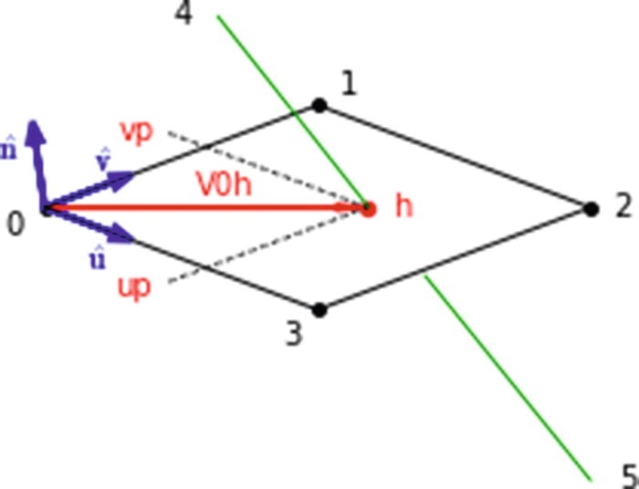
Out-of-bounds geometry

To find up, you project V0h onto the 03 direction. To do that, you take the dot product of V0h with û:
$$ up=acdotp ux+bcdotp uy+ccdotp uz $$
(5-48)
To find vp, you take the dot product of V0h with $$ widehat{mathbf{v}} $$:
$$ vp=acdotp vx+bcdotp vy+ccdotp vz $$
(5-49)
If you regard the line from 4 to 5 as being finite, you can test to see if it is long enough to reach the plane. From Figure 5-1,
$$ a= xh-xleft[4
ight] $$
(5-50)
$$ b= yh-yleft[4
ight] $$
(5-51)
$$ c= zh-zleft[4
ight] $$
(5-52)
$$ Q4h=sqrt{a^2+{b}^2+{c}^2} $$
(5-53)
if Q45 < Qh    LINE TOO SHORT, NO HIT

All of this has been incorporated in Listing 5-1, which has the same structure as Listing 3-5 in Chapter 3, although some of the functions and operations have been altered. As in that program, rotation directions and amounts are entered through the keyboard. Rotations are additive; for example, if the system is rotated first by Rx=40 degrees, followed by Rx=10, the total angle will be 50 degrees. Ry and Rz operate similarly.

Some data is hard-wired in Listing 5-1, such as definitions of the rectangular plane and the line intersecting it. They are shown in the lists in lines 18–20. There are six elements in each list numbered [0]-[5]: [0]-[3] are the four corners of the plane while [4] and [5] are the beginning and end of the line. They are coordinated with the diagrams in Figures 5-1 and 5-2. To modify the plane and line, just put new numbers in the lists. For example, item [5] is the end of the line. To drop it down in the +y direction, increase y[5]. The numbers in the lists are in local coordinates relative to the center of rotation (xc,yc,zc), which is at the center of the plane. The values are shown in Lines 14-16.

It takes only three points to define a plane. Here you have a four-corner rectangular plane. If you alter the plane’s corner coordinates, be sure they lie in the same plane. The easiest way to do so is to start off with a plane that lies in or is parallel to one of the coordinate planes. It can be rotated out of that coordinate plane later. In line 19, the first four elements of the y list are all zero. That describes a flat plane parallel to the x,z plane at y=0. Also, if altering the [x] or [z] lists, be sure the plane remains rectangular since the calculations of the hit point in this analysis assume that is the case.

Rotation functions rotx, roty, and rotz, which rotate coordinates around the coordinate directions, are included in lines 28-35. They are the same as used in prior programs so they have not been listed.

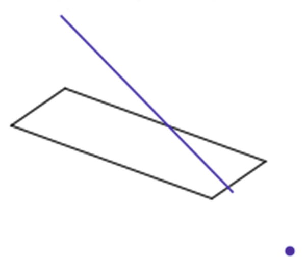
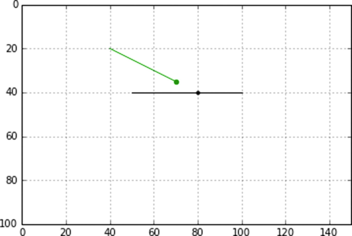
Line 45 plots a dot at the hit point (xhg,yhg) where the line intersects the plane. If the hit point lies within the plane’s boundaries, the color of the dot is red; if it’s outside, it is blue. If the line from [4] to [5] is too short and never reaches the plane, the color is changed to green and a dot is placed at [5], the end of the line. This is illustrated in Figure 5-5. The calculation of the hit point is carried out by function hitpoint(x,y,z), which begins in line 53. The program follows the analysis above in Equations 5-1 through 5-49 and should be self-explanatory.

Data input takes place in lines 154-166. This is similar to Listing 3-5. Samples of the output are shown in Figures 5-3, 5-4, and 5-5. Parameters are included in the captions.
../images/456962_1_En_5_Chapter/456962_1_En_5_Fig3_HTML.jpg
Figure 5-3

Line intersecting the plane defined by a rectangle. The hit point lies within the plane’s boundaries: y[5]=+5, Rx=45°, Ry=45°, Rz°=20

../images/456962_1_En_5_Chapter/456962_1_En_5_Fig4_HTML.jpg
Figure 5-4

Line intersecting the plane defined by a rectangle. The hit point lies outside the rectangle’s boundaries: y[5]=-5, Rx=45°, Ry=45°, Rz°=20.

../images/456962_1_En_5_Chapter/456962_1_En_5_Fig5_HTML.jpg
Figure 5-5

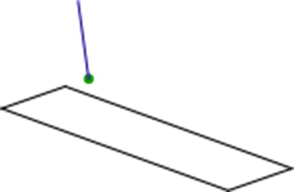
Example of a line too short, in which case a green dot appears at coordinate [5]: x[4]=-40, y[4]=-20, z[4]=15, x[5]=-20, y[5]=-10, z[5]=0, Rx=30°, Ry=45°, Rz°=20

1   """
2   LRP
3   """
4
5   import numpy as np
6   import matplotlib.pyplot as plt
7   from math import sin, cos, radians,sqrt
8
9   #——————————————fill lists with starting coordinates
10  xg=[ ]
11  yg=[ ]
12  zg=[ ]
13
14  xc=80 #————————center coordinates
15  yc=40
16  zc=40
17
18  x=[-40,-40,40,40,-40,50] #—system (plane and line geometry)
19  y=[0,0,0,0,-20,3]
20  z=[-10,10,10,-10,15,-10]
21
22  for i in range(len(x)):
23        xg.append(x[i]+xc)
24        yg.append(y[i]+yc)
25        zg.append(z[i]+zc)
26
27  #——————————————————define  rotation  functions
28  def rotx(xc,yc,zc,xp,yp,zp,Rx):
29       (same as in prior programs)
30
31  def  roty(xc,yc,zc,xp,yp,zp,Ry):
32        (same as in prior programs)
33
34  def rotz(xc,yc,zc,xp,yp,zp,Rz):
35       (same as in prior programs)
36
37  #———————————————-plot  plane, line and hit point
38  def plotsystem(xg,yg,zg,xh,yh,xhg,yhg,hitcolor):
39       plt.plot([xg[0],xg[1]],[yg[0],yg[1]],color='k')  #—————plot plane
40       plt.plot([xg[1],xg[2]],[yg[1],yg[2]],color='k')
41       plt.plot([xg[2],xg[3]],[yg[2],yg[3]],color='k')
42       plt.plot([xg[3],xg[0]],[yg[3],yg[0]],color='k')
43       plt.plot([xg[4],xg[5]],[yg[4],yg[5]],color='b') #———plot line
44
45       if hitcolor="g": #——————plot hit point at [5]
46             plot.scatter(xg[5],yg[5],s=20,color=hitcolor)
47       else: #——————plot hit point at h
48             plt.scatter(xhg,yhg,s=20,color=hitcolor)
49
50       plt.axis([0,150,100,0]) #———replot axes and grid
51       plt.axis('on')
52       plt.grid(False)
53       plt.show() #———plot latest rotation
54
55  #—————————————find hit point coordinates and color
56  def hitpoint(x,y,z):
57       a=x[5]-x[4]
58       b=y[5]-y[4]
59       c=z[5]-z[4]
60       Q45=sqrt(a*a+b*b+c*c)  #———distance  point  4  to  5
61
62       lx=a/Q45 #———unit vector components point 4 to 5
63       ly=b/Q45
64       lz=c/Q45
65
66       a=x[3]-x[0]
67       b=y[3]-y[0]
68       c=z[3]-z[0]
69       Q03=sqrt(a*a+b*b+c*c) #———distance 0 to 3
70
71       ux=a/Q03 #———unit vector 0 to 3
72       uy=b/Q03
73       uz=c/Q03
74
75       a=x[1]-x[0]
76       b=y[1]-y[0]
77       c=z[1]-z[0]
78       Q01=sqrt(a*a+b*b+c*c) #———distance 0 to 1
79
80       vx=a/Q01 #———unit vector 0 to 1
81       vy=b/Q01
82       vz=c/Q01
83
84       nx=uy*vz-uz*vy #———normal unit vector
85       ny=uz*vx-ux*vz
86       nz=ux*vy-uy*vx
87
88       vx1b=x[4]-x[0] #———vector components 0 to 4
89       vy1b=y[4]-y[0]
90       vz1b=z[4]-z[0]
91
92       Qn=(vx1b*nx+vy1b*ny+vz1b*nz) #———perpendicular distance 4 to plane
93
94       cosp=lx*nx+ly*ny+lz*nz #——cos of angle p
95       Qh=abs(Qn/cosp) #———distance 4 to hit point
96
97       xh=x[4]+Qh*lx  #———hit  point  coordinates
98       yh=y[4]+Qh*ly
99       zh=z[4]+Qh*lz
100
101      xhg=xh+xc #———global hit point coordinates
102      yhg=yh+yc
103      zhg=zh+zc
104
105  #————————————————————out of bounds check
106      a=xh-x[0] #——components of vector V0h
107      b=yh-y[0]
108      c=zh-z[0]
109
110      up=a*ux+b*uy+c*uz #———dot products
111      vp=a*vx+b*vy+c*vz
112
113      hitcolor='r' #———if inbounds plot red hit point
114      if up<0: #———change color to blue if hit point out of bounds
115           hitcolor='b'
116
117      if up>Q03:
118           hitcolor='b'
119
120      if vp<0:
121           hitcolor='b'
122
123      if vp>Q01:
124           hitcolor='b'
125
126      a=x[5]-x[4]
127      b=y[5]-y[4]
128      c=z[5]-z[4]
129      Q45=sqrt(a*a+b*b+c*c)
130
131      if Q45 < Qh:
132           hitcolor='g'
133
134      return xh,yh,xhg,yhg,hitcolor
135
136 #————————————————transform  coordinates  and  plot
137 def  plotx(xc,yc,zc,Rx):   #———transform  &  plot  Rx  system
138       for i in range(len(x)):
139             [xg[i],yg[i],zg[i]]=rotx(xc,yc,zc,x[i],y[i],z[i],Rx)
140             [x[i],y[i],z[i]]=[xg[i]-xc,yg[i]-yc,zg[i]-zc]
141
142       xh,yh,xhg,yhg,hitcolor=hitpoint(x,y,z) #———returns xh,yh,xhg,yhg
143
144       plotsystem(xg,yg,zg,xh,yh,xhg,yhg,hitcolor) #———plot
145
146 def ploty(xc,yc,zc,Ry):  #———transform & plot Ry system
147      for i in range(len(x)):
148            [xg[i],yg[i],zg[i]]=roty(xc,yc,zc,x[i],y[i],z[i],Ry)
149            [x[i],y[i],z[i]]=[xg[i]-xc,yg[i]-yc,zg[i]-zc]
150
151      xh,yh,xhg,yhg,hitcolor=hitpoint(x,y,z)
152
153      plotsystem(xg,yg,zg,xh,yh,xhg,yhg,hitcolor)
154
155 def plotz(xc,yc,zc,Rz):   #———transform  &  plot  Rz  system
156      for i in range(len(x)):
157            [xg[i],yg[i],zg[i]]=rotz(xc,yc,zc,x[i],y[i],z[i],Rz)
158            [x[i],y[i],z[i]]=[xg[i]-xc,yg[i]-yc,zg[i]-zc]
159
160      xh,yh,xhg,yhg,hitcolor=hitpoint(x,y,z)
161
162      plotsystem(xg,yg,zg,xh,yh,xhg,yhg,hitcolor)
163
164 #—————————————————-input data and plot system
165 while True:
166      axis=input('x, y or z?: ') #———input axis of rotation (lower case)
167      if axis == 'x': #—if x axis
168            Rx=radians(float(input('Rx Degrees?: '))) #———input degrees
169            plotx(xc,yc,zc,Rx) #–call function plotx
170      if axis == 'y':
171            Ry=radians(float(input('Ry Degrees?: '))) #———input degrees
172            ploty(xc,yc,zc,Ry)
173      if axis == 'z':
174            Rz=radians(float(input('Rz Degrees?: '))) #———input degrees
175            plotz(xc,yc,zc,Rz)
176      if axis == ":
177            break #—quit the program
Listing 5-1

Program LRP

5.2 Line Intersecting a Triangular Plane

Almost any flat surface can be formed by an array of triangular planes and a curved surface can be approximated by triangles, hence our interest in triangular planes .

Figure 5-6 shows the geometry for a line intersecting a triangular plane. The algorithms used in Listing 5-3 are mostly the same as in Listing 5-1. One difference is that the lengths of the list are, of course, shorter since the triangle has one less corner. Another is that the check on whether the hit point lies within the triangle or is out of bounds is different.

Before going on to Listing 5-3, you will develop a simple way to determine if a hit point lies within a triangle or outside of it. Figure 5-7 shows the geometry used for the out-of-bounds calculation. Listing 5-2 produces the output shown in Figure 5-8 and, with modification to the lists defining the coordinates of point 3, in Figure 5-9. In Figure 5-8, the hit is out of bounds; in Figure 5-9, it is within the triangle.
../images/456962_1_En_5_Chapter/456962_1_En_5_Fig6_HTML.jpg
Figure 5-6

Geometry of a line intersecting a triangular plane

Figure 5-7 shows three triangles: the black one, defined by points 0, 1, and 2, is the base triangle, the one you are concerned with. It has area A. The triangle defined by points 0, 1, and 3 (the hit point) has area A1. The third triangle between point 0, 3, and 2 has area A2. It is easy to see that if A1+A2>A, the hit point is out of bounds; if A1+A2<A, it is in bounds. If you can calculate the areas of the three triangles, you will have an easy way to determine if the hit point is within or outside of the base triangle. To do so, you rely on a simple expression for determining the area of a triangle:
$$ s=left(a+b+c
ight)/2 $$
(5-54)
$$ A=sqrt{sleft(s-a
ight)kern0.1em left(s-b
ight)kern0.1em left(s-c
ight)} $$
(5-55)
where a, b, and c are the lengths of the three sides of the triangle and A is its area. This is known as Heron’s formula, named after Hero of Alexandria, a Greek engineer and mathematician circa 10 AD - 70 AD.

This relation is put to use in Listing 5-2 and later in Listing 5-3. In Listing 5-2, most of the program is concerned with evaluating the lengths of the lines shown in Figure 5-7. Heron’s formula is then used to calculate the three areas: A, A1, and A2. The decision whether the hit point is inside or outside of the base triangle is made in lines 114-117 of Listing 5-2. It produces Figure 5-8. Program THT2 (not shown) is the same as THT1 (Listing 5-2) but has the lists adjusted to put the hit point within the triangle. It produces Figure 5-9. The adjusted lists are

x=[40,30,80,55]

y=[60,10,60,45]

z=[0,0,0,0]

As you can see from these lists, the hit point has been moved to (55,45,0).
../images/456962_1_En_5_Chapter/456962_1_En_5_Fig7_HTML.jpg
Figure 5-7

Model for out-of-bounds test

../images/456962_1_En_5_Chapter/456962_1_En_5_Fig8_HTML.jpg
Figure 5-8

Out of bounds, no hit produced by Listing 5-2

../images/456962_1_En_5_Chapter/456962_1_En_5_Fig9_HTML.jpg
Figure 5-9

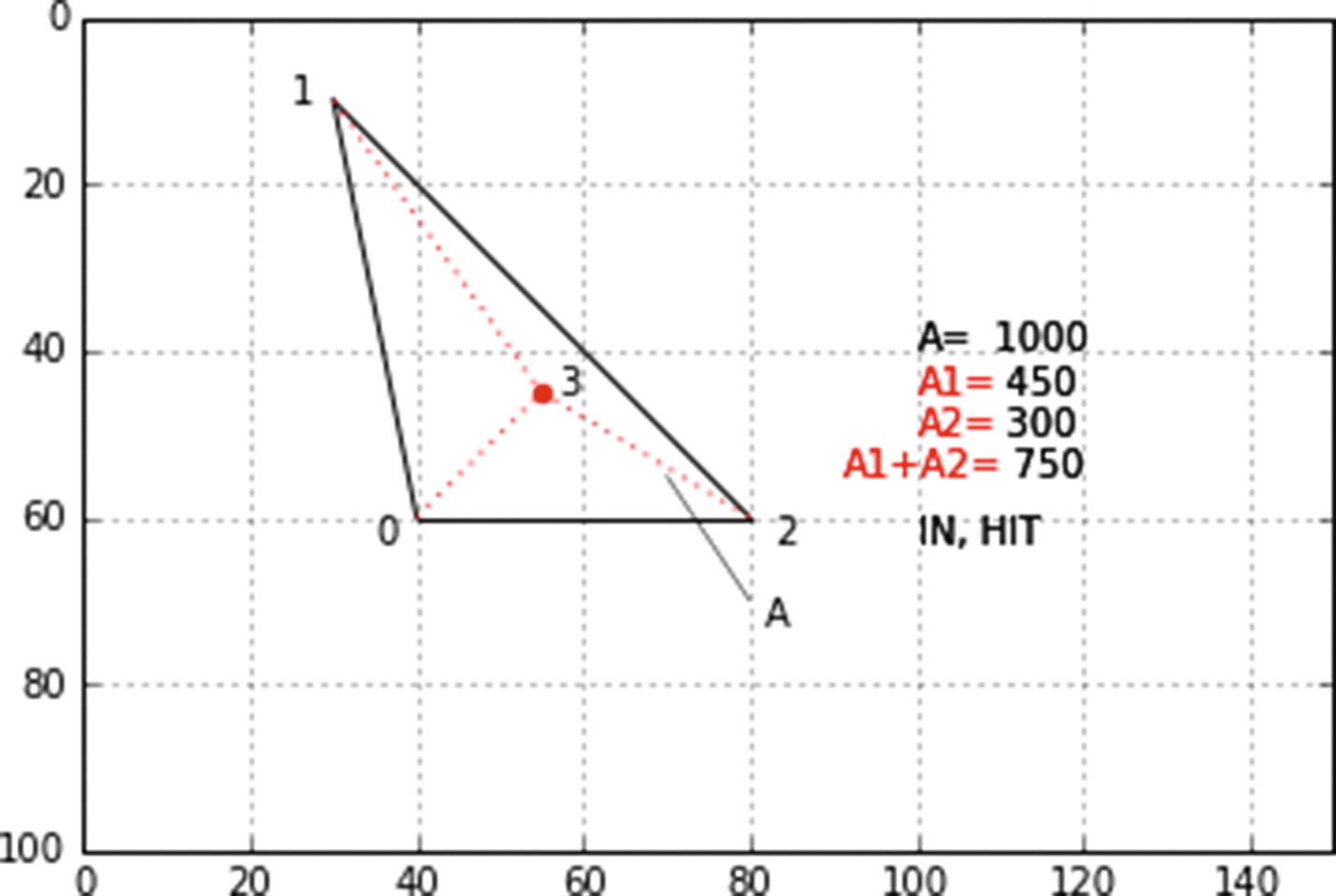
In bounds, hit produced by modified Listing 5-2

1   """
2   THT1
3   """
4
5   import matplotlib.pyplot as plt
6   import numpy as np
7   from math import sin, cos, radians, sqrt
8
9   plt.axis([0,150,100,0])
10
11  plt.axis('on')
12  plt.grid(True)
13
14  x=[40,30,80,75] #———plane
15  y=[60,10,60,40]
16  z=[0,0,0,0]
17
18  plt.plot([x[0],x[1]],[y[0],y[1]],color='k') #——plot plane A
19  plt.plot([x[1],x[2]],[y[1],y[2]],color='k')
20  plt.plot([x[2],x[0]],[y[2],y[0]],color='k')
21  plt.scatter(x[3],y[3],s=20,color='r')
22
23  plt.plot([x[0],x[3]],[y[0],y[3]],linestyle=':',color='r') #plot planes
24  plt.plot([x[1],x[3]],[y[1],y[3]],linestyle=':',color='r')
25  plt.plot([x[2],x[3]],[y[2],y[3]],linestyle=':',color='r')
26
27  plt.text(35,63,'0') #——label corners
28  plt.text(25,10,'1')
29  plt.text(83,63,'2')
30  plt.text(x[3]+2,y[3],'3')
31
32  a=x[1]-x[0] #——calculate dimensions
33  b=y[1]-y[0]
34  c=z[1]-z[0]
35  Q01=sqrt(a*a+b*b+c*c)
36
37  a=x[2]-x[1]
38  b=y[2]-y[1]
39  c=z[2]-z[1]
40  Q12=sqrt(a*a+b*b+c*c)
41
42  a=x[2]-x[0]
43  b=y[2]-y[0]
44  c=z[2]-z[0]
45  Q02=sqrt(a*a+b*b+c*c)
46
47  a=x[1]-x[3]
48  b=y[1]-y[3]
49  c=z[1]=z[3]
50  Q13=sqrt(a*a+b*b+c*c)
51
52  a=x[2]-x[3]
53  b=y[2]-y[3]
54  c=z[2]-z[3]
55  Q23=sqrt(a*a+b*b+c*c)
56
57  a=x[0]-x[3]
58  b=y[0]-y[3]
59  c=z[0]-z[3]
60  Q03=sqrt(a*a+b*b+c*c)
61
62  s=(Q01+Q12+Q02)/2 #——calculate areas A, A1 and A2
63  A=sqrt(s*(s-Q01)*(s-Q12)*(s-Q02))
64
65  s1=(Q01+Q03+Q13)/2
66  A1=sqrt(s1*(s1-Q01)*(s1-Q03)*(s1-Q13))
67
68  s2=(Q02+Q23+Q03)/2
69  A2=sqrt(s2*(s2-Q02 )*(s2-Q23)*(s2-Q03))
70
71  plt.arrow(70,55,10,15,linewidth=.5,color='grey') #——label area A
72  plt.text(82,73,'A',color='k')
73
74  plt.text(100,40,'A=') #——plot output
75  dle='%7.0f'%  (A)
76  dls=str(dle)
77  plt.text(105,40,dls)
78
79  plt.text(100,45,'A1=',color='r')
80  dle='%7.0f'% (A1)
81  dls=str(dle)
82  plt.text(105,45,dls)
83
84  plt.text(100,50,'A2=',color='r')
85  dle='%7.0f'% (A2)
86  dls=str(dle)
87  plt.text(105,50,dls)
88
89  plt.text(91,55,'A1+A2=',color='r')
90  dle='%7.0f'%  (A1+A2)
91  dls=str(dle)
92  plt.text(106,55,dls)
93
94  plt.text(100,40,'A=')
95  dle='%7.0f'%  (A)
96  dls=str(dle)
97  plt.text(105,40,dls)
98
99  plt.text(100,45,'A1=',color='r')
100 dle='%7.0f'% (A1)
101 dls=str(dle)
102 plt.text(105,45,dls)
103
104 plt.text(100,50,'A2=',color='r')
105 dle='%7.0f'% (A2)
106 dls=str(dle)
107 plt.text(105,50,dls)
108
109 plt.text(91,55,'A1+A2=',color='r')
110 dle="%7.0f'% (A1+A2)
111 dls=str(dle)
112 plt.text(106,55,dls)
113
114 if A1+A2 > A:
115      plt.text(100,63,'OUT, NO HIT')
116 else:
117      plt.text(100,63,'IN, HIT')
118
119 plt.show()
Listing 5-2

Program THT1

Listing 5-3 plots the hit point between a line and a triangle. It is similar to Listing 5-1 except it uses the inside or outside test developed above. Examples of output are shown in Figures 5-10, 5-11, and 5-12. One difference worth noting is in the calculation of the unit vector $$ widehat{mathbf{n}} $$, which is perpendicular to the plane of the triangle. In Listing 5-1, this was found by taking the cross product of û with vˆ. Since the angle between û and $$ widehat{mathbf{v}} $$ was 90 ° , this produced a unit vector that was normal to both of them, which implies normal to the plane, and of magnitude 1. This is because $$ left|widehat{mathbf{u}}	imes widehat{mathbf{v}}
ight|=left|widehat{mathbf{u}}
ight|kern0.1em left|widehat{mathbf{v}}
ight|kern0.1em sin left(alpha 
ight) $$ where α is the angle between û and $$ widehat{mathbf{v}} $$. When α equals 90 ° , $$ left|widehat{mathbf{u}}	imes widehat{mathbf{v}}
ight|=(1)(1)(1)=1 $$.
../images/456962_1_En_5_Chapter/456962_1_En_5_Fig10_HTML.jpg
Figure 5-10

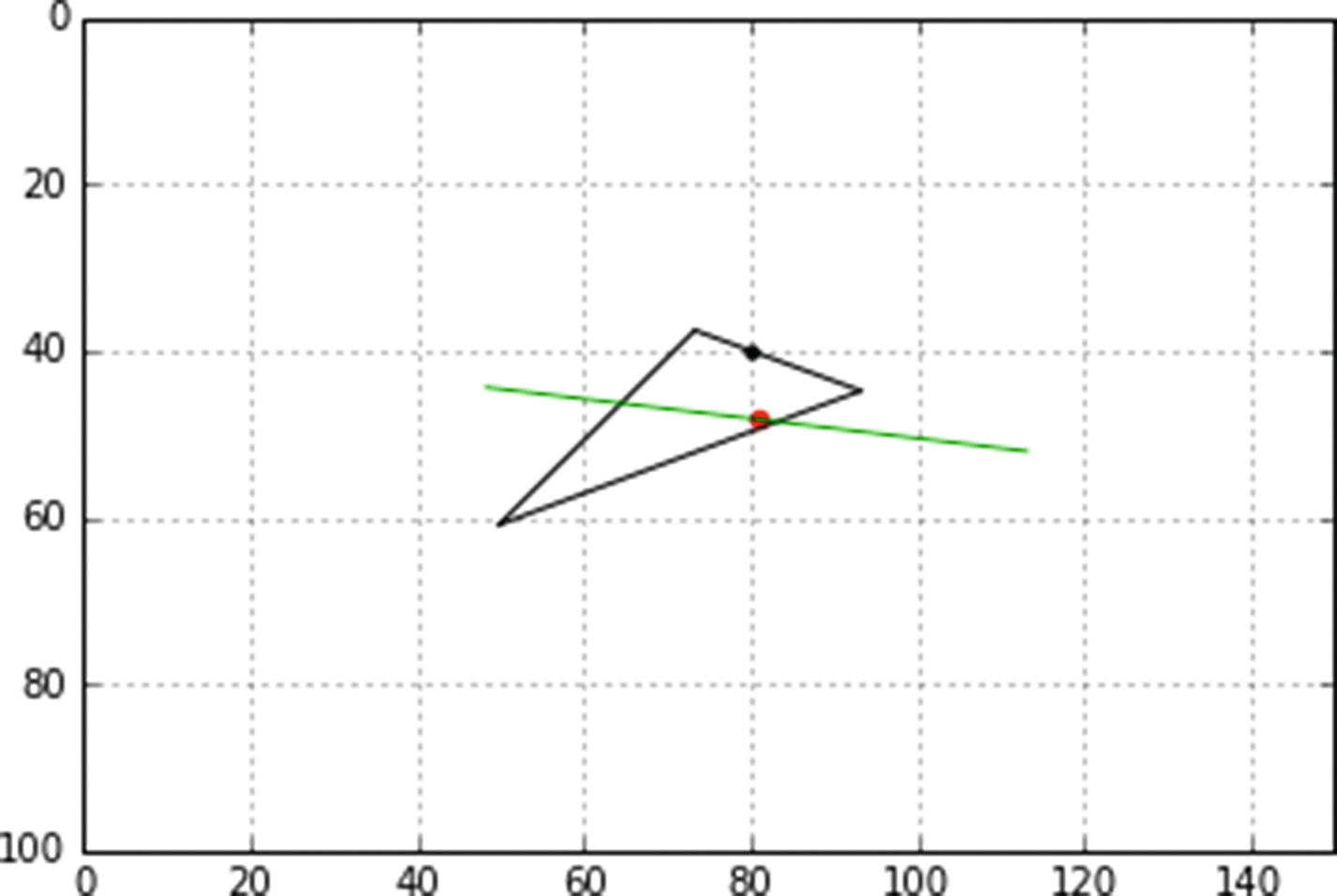
In-bounds hit. x[3]=-60, x[4]=70, y[3]=-20, y[4]=20, z[3]=15, z[4]=0, Rx=-90, Ry=45, Rz=20 (produced by Listing 5-3)

../images/456962_1_En_5_Chapter/456962_1_En_5_Fig11_HTML.jpg
Figure 5-11

Out-of-bounds hit. x[3]=-60, x[4]=40, y[3]=-20, y[4]=5, z[3]=15, z[4]=0, Rx=-90, Ry=45, Rz=20 (produced by Listing 5-3)

../images/456962_1_En_5_Chapter/456962_1_En_5_Fig12_HTML.jpg
Figure 5-12

Line too short, no hit. x[3]=-40, x[4]=-10, y[3]=-20, y[4]=-5, z[3]=15, z[4]=0, Rx=0, Ry=0, Rz=0 (produced by Listing 5-3)

However, with a general non-right triangle, the angle is not 90 ° so the vector resulting from the cross product, while normal to the plane, does not have a value of 1; in other words, it is not a unit vector. The algorithm between lines 88 and 91 makes the correction by normalizing $$ widehat{mathbf{n}} $$’s components. It does this by dividing each of them by the magnitude of $$ widehat{mathbf{n}} $$. In line 88, magn is the magnitude of $$ widehat{mathbf{n}} $$ before normalization of the vector’s components. Depending on the angle α, its value will be somewhere between 0 and 1. Dividing each component of $$ widehat{mathbf{n}} $$ by magn makes $$ widehat{mathbf{n}} $$ a unit vector.

1   """
2   LTP
3   """
4
5   import numpy as np
6   import matplotlib.pyplot as plt
7   from math import sin, cos, radians,sqrt
8
9   #——————————————fill lists with starting coordinates
10  xg=[ ]
11  yg=[ ]
12  zg=[ ]
13
14  xc=80 #————————center coordinates
15  yc=40
16  zc=40
17
18  x=[-10,-30,20,-40,-10]
19  y=[0,0,0,-20,-5]
20  z=[0,30,0,15,0]
21
22  for i in range(len(x)):
23        xg.append(x[i]+xc)
24        yg.append(y[i]+yc)
25        zg.append(z[i]+zc)
26
27  #—————————————————–define  rotation  functions
28  def rotx(xc,yc,zc,xp,yp,zp,Rx):
29       (same as in prior programs)
30
31  def  roty(xc,yc,zc,xp,yp,zp,Ry):
32       (same as in prior programs)
33
34  def rotz(xc,yc,zc,xp,yp,zp,Rz):
35       (same as in prior programs)
36
37  #———————————————-define  system  plotting  functions
38  def plotsystem(xg,yg,zg,xh,yh,xhg,yhg,hitcolor):
39       plt.plot([xg[0],xg[1]],[yg[0],yg[1]],color='k')  #—————plot plane
40       plt.plot([xg[1],xg[2]],[yg[1],yg[2]],color='k')
41       plt.plot([xg[2],xg[0]],[yg[2],yg[0]],color='k')
42       plt.plot([xg[3],xg[4]],[yg[3],yg[4]],color='g') #———plot line
43       plt.scatter(xc,yc,s=10,color='k') #———plot center of rotation
44
45       if hitcolor=='g':
46            plt.scatter(xg[4],yg[4],s=20,color=hitcolor)
47       else:
48            plt.scatter(xhg,yhg,s=20,color=hitcolor) #——————plot hit point
49
50       plt.axis([0,150,100,0]) #———replot axes and grid
51       plt.axis('on')
52       plt.grid(True)
53       plt.show() #———plot latest rotation
54
55  #————————————-calculate hit point coordinates and color
56  def hitpoint(x,y,z):
57       a=x[4]-x[3]
58       b=y[4]-y[3]
59       c=z[4]-z[3]
60       Q34=sqrt(a*a+b*b+c*c)  #———distance point 3 to 4
61
62       lx=a/Q34 #———unit vector components point 3 to 4
63       ly=b/Q34
64       lz=c/Q34
65
66       a=x[2]-x[0]
67       b=y[2]-y[0]
68       c=z[2]-z[0]
69       Q02=sqrt(a*a+b*b+c*c) #———distance 0 to 3
70
71       ux=a/Q02 #———unit vector 0 to 3
72       uy=b/Q02
73       uz=c/Q02
74
75       a=x[1]-x[0]
76       b=y[1]-y[0]
77       c=z[1]-z[0]
78       Q01=sqrt(a*a+b*b+c*c) #———distance 0 to 1
79
80       vx=a/Q01 #———unit vector 0 to 1
81       vy=b/Q01
82       vz=c/Q01
83
84       nx=uy*vz-uz*vy #———normal unit vector
85       ny=uz*vx-ux*vz
86       nz=ux*vy-uy*vx
87  #——————————–correct magnitude of unit vector ^n
88       magn=sqrt(nx*nx+ny*ny+nz*nz)
89       nx=nx/magn
90       ny=ny/magn
91       nz=nz/magn
92  #——————————————————————
93       a=x[3]-x[0] #———vector components 0 to 3
94       b=y[3]-y[0]
95       c=z[3]-z[0]
96
97       Qn=(a*nx+b*ny+c*nz) #———perpendicular distance 3 to plane
98
99       cosp=lx*nx+ly*ny+lz*nz #———cos of angle p
100      Qh=abs(Qn/cosp) #———distance 4 to hit point
101
102      xh=x[3]+Qh*lx #———hit point coordinates
103      yh=y[3]+Qh*ly
104      zh=z[3]+Qh*lz
105
106      xhg=xh+xc #———global hit point coordinates
107      yhg=yh+yc
108      zhg=zh+zc
109
110 #————————————————————out of bounds check
111      a=x[1]-x[2]
112      b=y[1]-y[2]
113      c=z[1]-z[2]
114      Q12=sqrt(a*a+b*b+c*c)
115
116      a=x[1]-xh
117      b=y[1]-yh
118      c=z[1]-zh
119      Q1h=sqrt(a*a+b*b+c*c)
120
121      a=x[2]-xh
122      b=y[2]-yh
123      c=z[2]-zh
124      Q2h=sqrt(a*a+b*b+c*c)
125
126      a=x[0]-xh
127      b=y[0]-yh
128      c=z[0]-zh
129      Q0h=sqrt(a*a+b*b+c*c)
130
131      s=(Q01+Q12+Q02)/2 #—area A
132      A=sqrt(s*(s-Q01)*(s-Q12)*(s-Q02))
133
134      s1=(Q01+Q0h+Q1h)/2 #———area A1
135      A1=sqrt(s1*(s1-Q01)*(s1-Q0h)*(s1-Q1h))
136
137      s2=(Q02+Q2h+Q0h)/2 #—area A2
138      A2=sqrt(s2*(s2-Q02)*(s2-Q2h)*(s2-Q0h))
139
140      hitcolor='r' #———if within bounds plot red hit point
141
142      if A1+A2 > A: #———if out of bounds plot blue hit point
143           hitcolor='b'
144
145      a=x[4]-x[3]
146      b=y[4]-y[3]
147      c=z[4]-z[3]
148      Q34=sqrt(a*a+b*b+c*c)
149
150      if Q34 < Qh: #———if line too short plot green at end of line
151           hitcolor='g'
152
153      return xh,yh,xhg,yhg,hitcolor
154
155 #————————————————transform coordinates and plot
156 def plotx(xc,yc,zc,Rx):   #———transform & plot Rx system
157      for i in range(len(x)):
158            [xg[i],yg[i],zg[i]]=rotx(xc,yc,zc,x[i],y[i],z[i],Rx)   
159            [x[i],y[i],z[i]]=[xg[i]-xc,yg[i]-yc,zg[i]-zc]
160
161      xh,yh,xhg,yhg,hitcolor=hitpoint(x,y,z) #———returns xh,yh,xhg,yhg
162
163      plotsystem(xg,yg,zg,xh,yh,xhg,yhg,hitcolor) #———plot plane, line, hit point
164
165      def ploty(xc,yc,zc,Ry):  #———transform & plot Ry system
166      for i in range(len(x)):
167           [xg[i],yg[i],zg[i]]=roty(xc,yc,zc,x[i],y[i],z[i],Ry)
168           [x[i],y[i],z[i]]=[xg[i]-xc,yg[i]-yc,zg[i]-zc]
169
170      xh,yh,xhg,yhg,hitcolor=hitpoint(x,y,z)
171
172      plotsystem(xg,yg,zg,xh,yh,xhg,yhg,hitcolor)
173
174 def plotz(xc,yc,zc,Rz):   #———transform  &  plot  Rz  system
175      for i in range(len(x)):
176            [xg[i],yg[i],zg[i]]=rotz(xc,yc,zc,x[i],y[i],z[i],Rz)
177            [x[i],y[i],z[i]]=[xg[i]-xc,yg[i]-yc,zg[i]-zc]
178
179      xh,yh,xhg,yhg,hitcolor=hitpoint(x,y,z)
180
181      plotsystem(xg,yg,zg,xh,yh,xhg,yhg,hitcolor)
182
183 #——————————————————input data and plot system
184      while True:
185           axis=input('x, y or z?: ') #———input axis of rotation (lower case)
186           if axis == 'x': #—if x axis
187                     Rx=radians(float(input('Rx Degrees?: '))) #———input degrees of rotation
188                     plotx(xc,yc,zc,Rx) #–call function plotx
189           if axis == 'y':
190                     Ry=radians(float(input('Ry Degrees?: '))) #———input degrees of rotation
191                     ploty(xc,yc,zc,Ry)
192           if axis == 'z':
193                     Rz=radians(float(input('Rz Degrees?: '))) #———input degrees of rotation
194                     plotz(xc,yc,zc,Rz)
195           if axis == ":
196                     break #———quit the program
Listing 5-3

Program LTP

5.3 Line Intersecting a Circle

The determination of whether the hit point of a line intersecting the plane of a circle is within the circle is trivial. As shown in Figure 5-13, if the distance from the circle’s center to the hit point is greater than the circle’s radius, it lies outside the circle:

if rh > r    NO HIT
../images/456962_1_En_5_Chapter/456962_1_En_5_Fig13_HTML.jpg
Figure 5-13

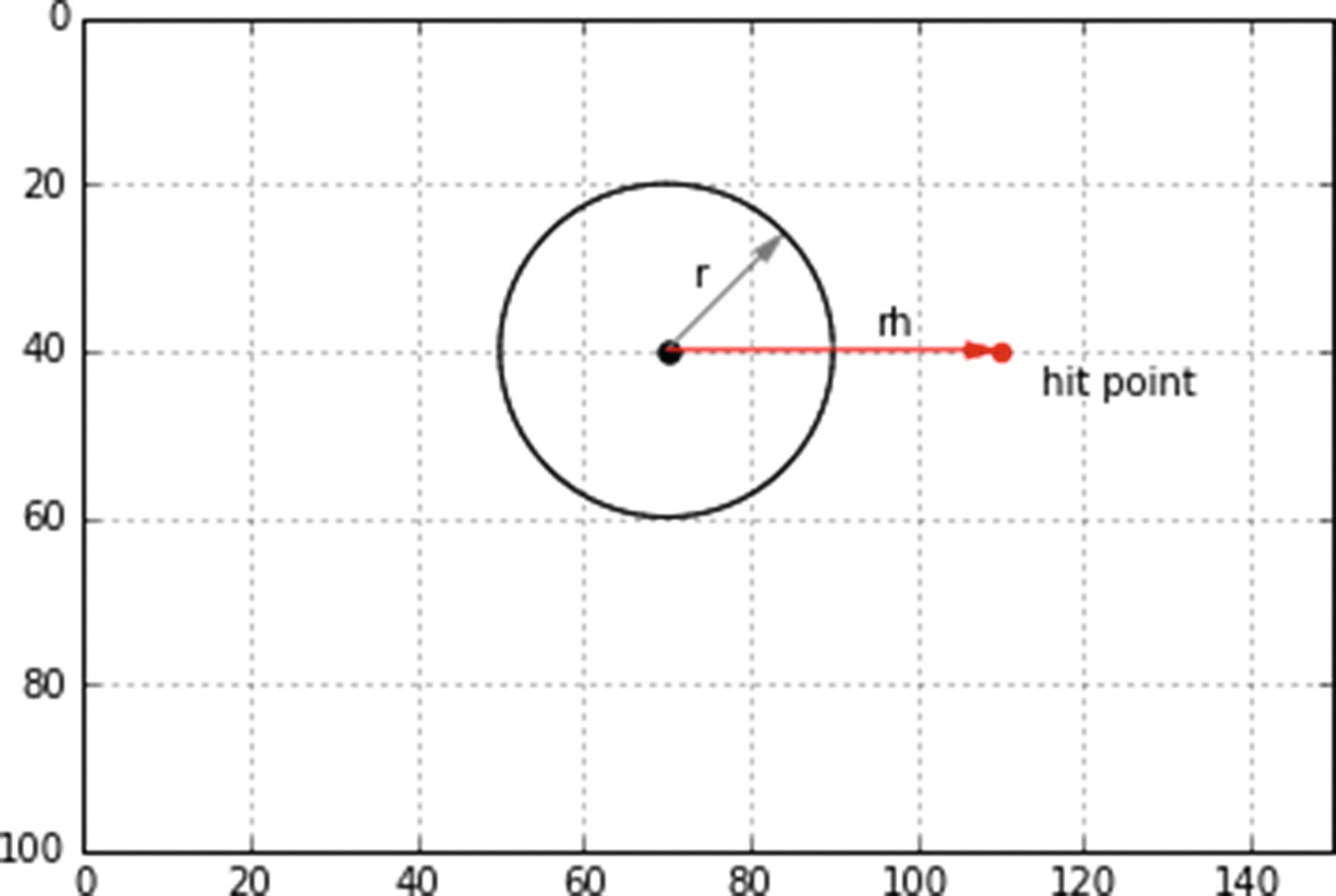
Model for out-of-bounds test for a circle

We won’t bother writing a separate program to demonstrate this. You should be able to do that yourself by modifying Listing 5-1 or Listing 5-3. Simply fill the x[ ],y[ ], and z[ ] lists with the points defining the circle’s perimeter and the line coordinates and modify the functions plotsystem and hitpoint.

5.4 Line Intersecting a Circular Sector

In this section, you develop a procedure to determine if the hit point of a line intersecting the plane of a sector of a circle is inside or outside the sector. Figure 5-14 shows the sector. It has a center at point 0 and a radius r. The hit point is at 3. rh is the distance from 0 to the hit point. Your goal is to determine if the hit point lies inside or outside the sector. (We will not be developing a full three-dimensional program here; you’ll just see how the inside or outside algorithm works.) It could be easily incorporated into any of the preceding programs, such as Listing 5-3.
../images/456962_1_En_5_Chapter/456962_1_En_5_Fig14_HTML.jpg
Figure 5-14

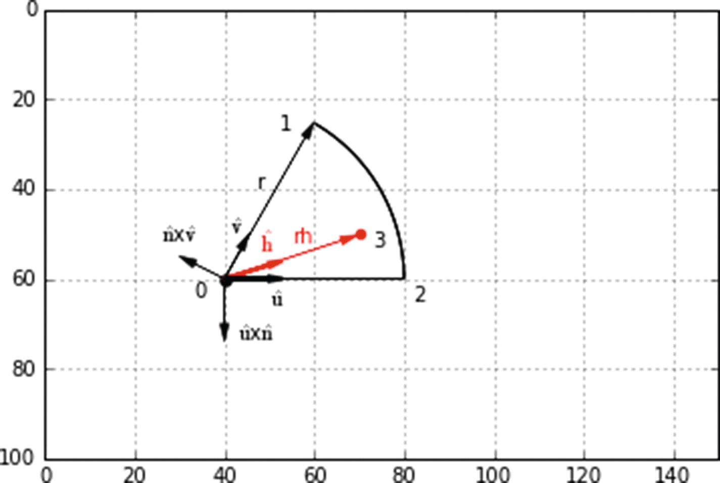
Model for determining whether a line intersecting a circular sector is in or out of bounds. 3=hit point.

There are five unit vectors at point 0: û points from 0 to 2; $$ widehat{mathbf{v}} $$ points from 0 to 1; and ĥ from 0 to the hit point at 3. $$ widehat{mathbf{n}} $$ is a unit vector normal to the plane of the sector. It is not shown since it points up and out of the plane. $$ widehat{mathbf{u}}	imes widehat{mathbf{n}} $$ is the result of the cross product of û with $$ widehat{mathbf{n}} $$; $$ widehat{mathbf{n}}	imes widehat{mathbf{v}} $$ is from the cross product of $$ widehat{mathbf{n}} $$ with $$ widehat{mathbf{v}} $$.

Your strategy is to first determine if Rh>r, in which case the hit point is outside the sector in the radial direction. Then you take the dot product of ĥ with $$ widehat{mathbf{u}}	imes widehat{mathbf{n}} $$. If the result is positive, the hit point is outside the sector on the 0-2 side. Then you take the dot product of ĥ with $$ widehat{mathbf{n}}	imes widehat{mathbf{v}} $$. If it is positive, the hit point is out of bounds on the 0-1 side.

In Listing 5-4, the local coordinates (relative to point 0) are defined in the lists in lines 14-16. The last element in the lists defines the coordinates of the hit point, point 3. xc,yc, and zc in lines 18-20 are the global coordinates of point 0. The hit test algorithm begins in line 23. Most of it should be self-explanatory based on the previous discussion. Attention is called to lines 52-58. This is where the normal vector $$ widehat{mathbf{n}} $$ is evaluated by taking the cross product of û with $$ widehat{mathbf{v}} $$. As explained earlier, this produces a unit vector (magnitude 1) only if û and $$ widehat{mathbf{v}} $$ are perpendicular to one another. Since the angle between them in a general sector will not necessarily be 90 degrees, the vector must be normalized. That takes place in lines 55-58. The dot product of $$ widehat{mathbf{u}}	imes widehat{mathbf{n}} $$ with ĥ takes place in line 64, $$ widehat{mathbf{n}}	imes widehat{mathbf{v}} $$ with ĥ in line 70. Line 72 assumes the hit color is red, which means the hit is within the sector. If A is positive, it lies outside the sector, in which case the hit color is changed to blue in line 74. Lines 76 and 77 perform the same test for the other side of the sector. Lines 79 and 80 check for the hit point lying outside the sector in the radial direction. Figures 5-15 and 5-16 show two sample runs. You can move the hit point around yourself by changing the coordinates of point 3 in the lists in lines 14-15. You change only the x and y coordinates of the hit point since it is assumed to lie in the z=0 plane, as does the sector.
../images/456962_1_En_5_Chapter/456962_1_En_5_Fig15_HTML.jpg
Figure 5-15

In-bounds or out-of-bounds test produced by Listing 5-4: red=in, blue=out

../images/456962_1_En_5_Chapter/456962_1_En_5_Fig16_HTML.jpg
Figure 5-16

In-bounds or out-of-bounds test produced by Listing 5-4: red=in, blue=out

1   """
2    LCSTEST
3   """
4
5   import matplotlib.pyplot as plt
6   import numpy as np
7   from math import sin, cos, radians, degrees, sqrt, acos
8
9   plt.axis([0,150,100,0])
10
11  plt.axis('on')
12  plt.grid(True)
13
14  x=[0,20,40,5]
15  y=[0,-35,0,-25]
16  z=[0,0,0,0]
17
18  xc=40
19  yc=60
20  zc=0
21
22  #——————————————hit test
23  a=x[3]-x[0]
24  b=y[3]-y[0]
25  c=z[3]-z[0]
26  rh=sqrt(a*a+b*b+c*c)
27
28  a=x[3]-x[0]
29  b=y[3]-y[0]
30  c=z[3]-z[0]
31  Q0h=sqrt(a*a+b*b+c*c)
32  hx=a/Q0h #———unit vector 0 to hit point
33  hy=b/Q0h
34  hz=c/Q0h
35
36  a=x[2]-x[0]
37  b=y[2]-y[0]
38  c=z[2]-z[0]
39  Q02=sqrt(a*a+b*b+c*c)
40  ux=a/Q02 #———unit vector 0 to 3
41  uy=b/Q02
42  uz=c/Q02
43
44  a=x[1]-x[0]
45  b=y[1]-y[0]
46  c=z[1]-z[0]
47  Q01=sqrt(a*a+b*b+c*c)
48  vx=a/Q01 #———unit vector 0 to 1
49  vy=b/Q01
50  vz=c/Q01
51
52  a=uy*vz-uz*vy #———vector uˆxvˆ normal to plane
53  b=uz*vx-ux*vz
54  c=ux*vy-uy*vx
55  Quxv=sqrt(a*a*b*b+c*c) #———normalize uˆxvˆ
56  nx=a/Quxv
57  ny=b/Quxv
58  nz=c/Quxv
59
60  uxnx=uy*nz-uz*ny #———unit vector uˆxvˆ
61  uxny=uz*nx-ux*nz
62  uxnz=ux*ny-uy*nx
63
64  A=uxnx*hx+uxny*hy+uxnz*hz #———dot product uˆxvˆ with hˆ
65
66  nxvx=ny*vz-nz*vy #———unit vector uˆxvˆ
67  nxvy=nz*vx-nx*vz
68  nxvz=nx*vy-ny*vx
69
70  B=nxvx*hx+nxvy*hy+nxvz*hz #———dot product uˆxvˆ with hˆ
71
72  hitcolor='r'
73  if A>0:  #—out
74       hitcolor='b'
75
76  if B>0: #—out
77       hitcolor='b'
78
79  if rh>r: #—out
80      hitcolor='b'
81
82  plt.scatter(x[3]+xc,y[3]+yc,s=20,color=hitcolor)
83
84  #————————————-plot   arc
85  r=40
86  phi1=0
87  phi2=-radians(60)
88  dphi=(phi2-phi1)/180
89  xlast=xc+r
90  ylast=yc+0
91  for phi in np.arange(phi1,phi2,dphi):
92      x=xc+r*cos(phi)
93      y=yc+r*sin(phi)
94      plt.plot([xlast,x],[ylast,y],color='k')
95      xlast=x
96      ylast=y
97
98
99  #————————————-labels
100 print('rh=',rh)
101 print('r=',r)
102 plt.arrow(xc,yc,40,0)
103 plt.arrow(xc,yc,20,-35,linewidth=.5,color='k')
103 plt.text(33,61,'0')
104 plt.text(52,27,'1')
105 plt.text(82,65,'2')
106
107  plt.show()
Listing 5-4

Program LCSTEST

5.5 Line Intersecting a Sphere

Figure 5-17, output from Listing 5-5, shows a line intersecting a sphere . The entrance and exit points are shown in red. Figure 5-18 shows the model used by Listing 5-5. The line begins at B and ends at E.
../images/456962_1_En_5_Chapter/456962_1_En_5_Fig17_HTML.jpg
Figure 5-17

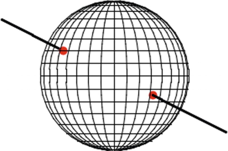
Line intersecting a sphere, produced by Listing 5-5

../images/456962_1_En_5_Chapter/456962_1_En_5_Fig18_HTML.jpg
Figure 5-18

Model for a line intersecting a sphere

To find the entrance hit point, you start at B and move a point p incrementally along the line toward E. At each step, you calculate Qpc, the distance between p and c. If it is less than or equal to the sphere’s radius rs, you have made contact with the sphere and a red dot is plotted. You continue moving p along the line inside the sphere without plotting anything (you could plot a dotted line), calculating Qpc as you go, until Qpc becomes equal to or greater than rs. At that point, p leaves the sphere and another red dot is plotted. p continues moving along the line to E, plotting black dots along the way. Instead of plotting the line with dots, you could have used short line segments as was done in prior programs.

To move p along the line, you use parameter t, which is the distance from B to p. To get the coordinates of p, you construct unit vector û, which points along the line
$$ a= xe- xb $$
(5-56)
$$ b= ye- yb $$
(5-57)
$$ c= ze- zb $$
(5-58)
$$ Qbe=sqrt{a^2+{b}^2+{c}^2} $$
(5-59)
$$ ux=a/ Qbe $$
(5-60)
$$ uy=b/ Qbe $$
(5-61)
$$ uz=c/ Qbe $$
(5-62)
where Qbe is the distance along the line from B to E and ux,uy, and uz are the components of û. The coordinates of p are thus
$$ xp= xb+ uxt $$
(5-63)
$$ yp= yb+ uyt $$
(5-64)
$$ zp= zb+ uzt $$
(5-65)
Qpc is easy to determine:
$$ a= xc- xp $$
(5-66)
$$ b= yc- yp $$
(5-67)
$$ c= zc- zp $$
(5-68)
$$ Qpc=sqrt{a^2+{b}^2+{c}^2} $$
(5-69)
In Listing 5-5, the sphere’s center coordinates are set in lines 18-20. The sphere is composed of longitude (vertical) lines and latitude (horizontal) lines. The lists in lines 10-16 contain the local and global coordinates of the longitudes. The initial filling of these lists takes place in lines 25-38, which create a half circle in the z=0 plane. As shown in Figure 5-19, point p lies on the circumference at coordinates xp,yp,zp where
$$ xp= rskern0.1em mathit{cos}left(phi 
ight) $$
(5-70)
$$ yp= rskern0.1em mathit{sin}left(phi 
ight) $$
(5-71)
$$ zp=0 $$
(5-72)

They are set in lines 30-32. ϕ is the angle around the z direction. It runs from -90 ° to +90 ° . You don’t need the back half of the longitudes so they are not plotted. This half circle will be rotated around the y direction to create the oval longitudes. They are 10 ° apart as set in line 74. Since they are rotated around the y direction only, the program contains just the rotation function roty: rotx and rotz are not needed in this model. Plotting of the longitudes takes place in lines 72-77.

The latitudes are plotted in lines 80-97. Figure 5-21 shows a front view of the sphere looking into the x,y plane. Each latitude is essentially a circle having radius rl where
$$ xl= rskern0.1em mathit{cos}left(phi 
ight) $$
(5-73)

This is calculated in line 89 of the program. When viewed from the front, the latitude appears as a straight line since you are not rotating the sphere in this program.

The ϕ loop beginning at line 88 ranges ϕ from -90 ° to + 90 ° in 10 ° increments. At each increment a new latitude is plotted. It will have a radius given by Equation 5-73 above. The α loop beginning at line 92 sweeps across the front of the circular latitude from α=0 ° to 180 ° in 10 ° increments. This is illustrated in Figure 5-22, which shows the top view looking down on the x,z plane.
../images/456962_1_En_5_Chapter/456962_1_En_5_Fig19_HTML.jpg
Figure 5-19

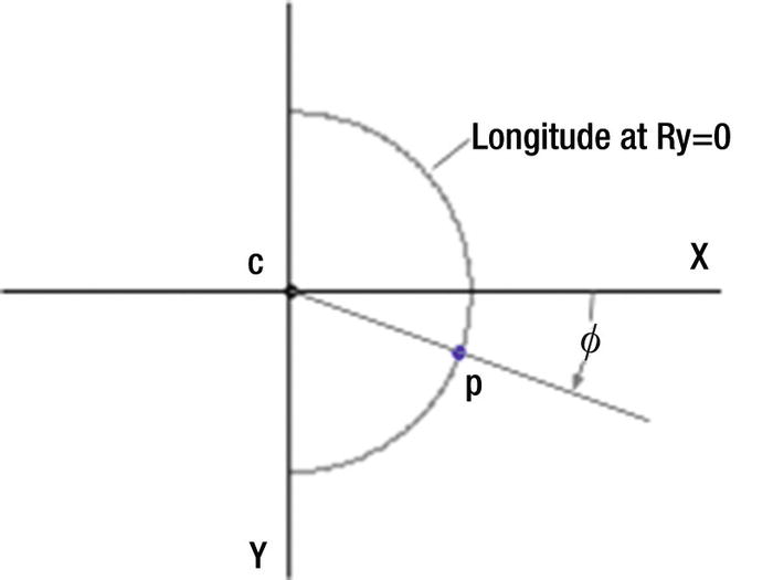
x,y view of sphere longitude shown at starting position Ry=0. Rotation around the y direction in 10° increments will produce longitudes.

../images/456962_1_En_5_Chapter/456962_1_En_5_Fig20_HTML.jpg
Figure 5-20

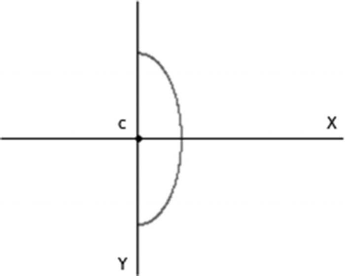
x,y view of sphere longitude rotated by Ry=60°

../images/456962_1_En_5_Chapter/456962_1_En_5_Fig21_HTML.jpg
Figure 5-21

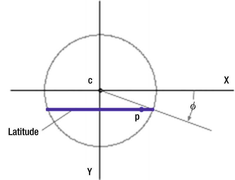
Sphere latitude - x,y view

../images/456962_1_En_5_Chapter/456962_1_En_5_Fig22_HTML.jpg
Figure 5-22

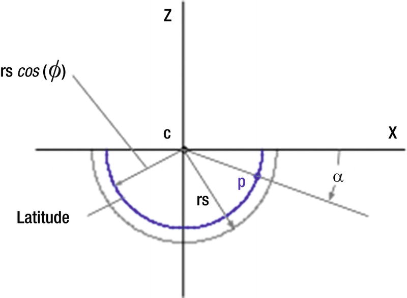
Sphere latitude - x,z view

1   """
2   LS
3   """
4
5   import numpy as np
6   import matplotlib.pyplot as plt
7   from math import sin, cos, radians, sqrt
8
9   #—————————————————————————lists
10  x=[ ]
11  y=[ ]
12  z=[ ]
13
14  xg=[ ]
15  yg=[ ]
16  zg=[ ]
17
18  xc=80 #——sphere center
19  yc=50
20  zc=0
21
22  rs=40 #———sphere radius
23
24  #————————————————————fill longitude lists
25  phi1=radians(-90)
26  phi2=radians(90)
27  dphi=radians(10)
28
29  for phi in np.arange(phi1,phi2,dphi):
30       xp=rs*cos(phi)
31       yp=rs*sin(phi)
32       zp=0
33       x.append(xp)
34       y.append(yp)
35       z.append(zp)
36       xg.append(xp)
37       yg.append(yp)
38       zg.append(zp)
39
40  #==============================================define rotation function
41  def roty(xc,yc,zc,xp,yp,zp,Ry):
42       a=[xp,yp,zp]
43       b=[cos(Ry),0,sin(Ry)] #———————[cx11,cx12,cx13]
44       xpp=np.inner(a, b)
45       b=[0,1,0] #—————[cx21,cx22,cx23]
46       ypp=np.inner(a,b) #——————–scalar product of a,b
47       b=[-sin(Ry),0,cos(Ry)] #—————[cx31,cx32,cx33]
48       zpp=np.inner(a,b)
49       [xg,yg,zg]=[xpp+xc,ypp+yc,zpp+zc]
50       return[xg,yg,zg]
51
52  #=========================================================
53  def plotsphere(xg,yg,zg):
54       lastxg=xg[0]
55       lastyg=yg[0]
56       for i in range(len(x)):
57             if i < len(x)/2:
58                   plt.plot([lastxg,xg[i]],[lastyg,yg[i]],linewidth=1,color='k')
59             else:
60                   plt.plot([lastxg,xg[i]],[lastyg,yg[i]],linewidth=1,color='k')
61       lastxg=xg[i]
62       lastyg=yg[i]
63
64  #================================================transform coordinates
65  def plotspherey(xc,yc,zc,Ry):
66       for i in range(len(x)): #—————transform and plot Ry sphere
67             [xg[i],yg[i],zg[i]]=roty(xc,yc,zc,x[i],y[i],z[i],Ry)
68
69  plotsphere(xg,yg,zg)  #———plot rotated coordinates
70
71  #—————————————————plot longitudes
72  Ry1=radians(0)
73  Ry2=radians(180)
74  dRy=radians(10)
75
76  for Ry in np.arange(Ry1,Ry2,dRy):
77       plotspherey(xc,yc,zc,Ry)
78
79  #————————————————–plot latitudes
80  alpha1=radians(0)
81  alpha2=radians(180)
82  dalpha=radians(10)
83
84  phi1=radians(-90)
85  phi2=radians(90)
86  dphi=radians(10)
87
88  for phi in np.arange(phi1,phi2,dphi):
89       r=rs*cos(phi) #————————latitude radius
90       xplast=xc+r
91       yplast=yc+rs*sin(phi)
92       for  alpha  in  np.arange(alpha1,alpha2,dalpha):
93            xp=xc+r*cos(alpha)
94            yp=yplast
95            plt.plot([xplast,xp],[yplast,yp],color='k')
96            xplast=xp
97            yplast=yp
98
99  #—————————————————line and hit points
100 xb=-60 #—line beginning
101 yb=-30
102 zb=-20
103
104 xe=60 #——line end
105 ye=30
106 ze=-40
107
108 a=xe-xb
109 b=ye-yb
110 c=ze-zb
111 Qbe=sqrt(a*a+b*b+c*c)  #———line length
112 ux=a/Qbe #—unit vector uˆ
113 uy=b/Qbe
114 uz=c/Qbe
115
116 dt=1
117 for t in np.arange(0,Qbe,dt):
118       xp=xb+ux*t
119       yp=yb+uy*t
120       zp=zb+uz*t
121       Qpc=sqrt(xp*xp+yp*yp+zp*zp)
122       if Qpc > rs:
123            plt.scatter(xp+xc,yp+yc,s=5,color='k')
124       if Qpc <= rs:
125            plt.scatter(xp+xc,yp+yc,s=80,color='r')
126       tlast=t
127       break
128
129 for t in np.arange(tlast,Qbe,dt):
130       xp=xb+ux*t
131       yp=yb+uy*t
132       zp=zb+uz*t
133       Qpc=sqrt(xp*xp+yp*yp+zp*zp)
134       if Qpc >= rs:
135            plt.scatter(xp+xc,yp+yc,s=80,color='r')
136       tlast=t
137       break
138
139 for t in np.arange(tlast,Qbe,dt):
140       xp=xb+ux*t
141       yp=yb+uy*t
142       zp=zb+uz*t
143       Qpc=sqrt(xp*xp+yp*yp+zp*zp)
144       if Qpc >= rs:
145            plt.scatter(xp+xc,yp+yc,s=5,color='k')
146
147 plt.axis([0,150,100,0]) #–plot axes and grid
148 plt.axis('off')
149 plt.grid(False)
150
151  plt.show()
Listing 5-5

Program LS

5.6 Plane Intersecting a Sphere

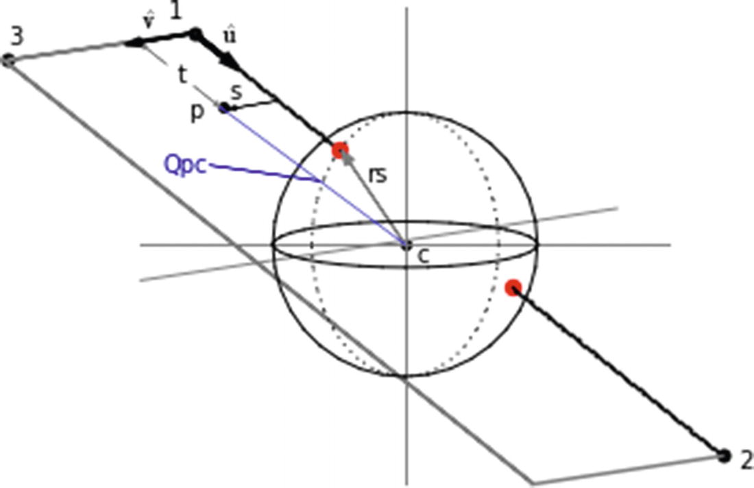
In this section, you will work out a technique for plotting a flat rectangular plane intersecting a sphere. Figure 5-23 shows the output of Listing 5-6; Figure 5-24 shows the model used by that listing.

The strategy here is to use the algorithms developed in the previous section for a line intersecting a sphere as your basic element. By representing the plane as a series of parallel lines, you can easily find the intersection of a plane with a sphere. Figure 5-23 shows unit vector û at corner 1. As before, this points from the beginning to end of the first line. There is also unit vector $$ widehat{mathbf{v}} $$ at corner 1. This points to corner 3. By advancing along the line from 1 to 3 in small steps, you can construct lines running parallel to the first one from 1 to 2. Advancing down each of these lines in small increments of t, you can find the coordinates of points across the plane. To advance in the $$ widehat{mathbf{v}} $$ direction, you introduce parameter s, which is the distance from corner 1 to the beginning of the new line. To get the coordinates of the end of that line, you perform the same operation starting at point 2 using vˆ and s, as in
$$ xe=x2+ vxcdotp s $$
(5-74)
$$ ye= yr+ vycdotp s $$
(5-75)
$$ ze=z2+ vzcdotp s $$
(5-76)
where xe, ye, and ze are the coordinates of the end of the line; x2,y2, and z2 are the coordinates of point 2; and vx,vy, and vz are the components of unit vector $$ widehat{mathbf{v}} $$.

Incrementing down and across the plane with parameters t and s allows you to sweep across the surface of the plane. At each point p you calculate the distance from p to the center of the sphere. If it is equal to or less than the sphere’s radius, you have a hit.

I won’t list the entire program that produced Figure 5-23 since it is mostly similar to Listing 5-5, except for the addition of an s loop that sweeps in the $$ widehat{mathbf{v}} $$ direction. Control of the program begins at line 27. Lines 27-37 define the coordinates of plane corners 1, 2, and 3. The unit vectors û and $$ widehat{mathbf{v}} $$ are established in lines 39-53. Lines 55 and 56 set the scan increments in dt and ds. The loop 57-64 scans in the $$ widehat{mathbf{v}} $$ direction, establishing the beginning and end coordinates of each line. Function plane, which begins at line 1, determines if there is a hit with each line and the sphere. For each s, the loop beginning at line 3 advances down the line in the û direction, calculating the coordinates xp,yp,zp of each point p along the line. Line 10 calculates the distance of p from the sphere’s center. Line 11 says, if the distance is greater than the sphere’s radius, plot a black dot. If it is less than or equal to the radius, line 18 plots a colorless dot. The rest of the logic up to line 24 determines if the line has emerged from the sphere, in which case plotting of black dots resumes. Results are shown in Figure 5-23.
../images/456962_1_En_5_Chapter/456962_1_En_5_Fig23_HTML.jpg
Figure 5-23

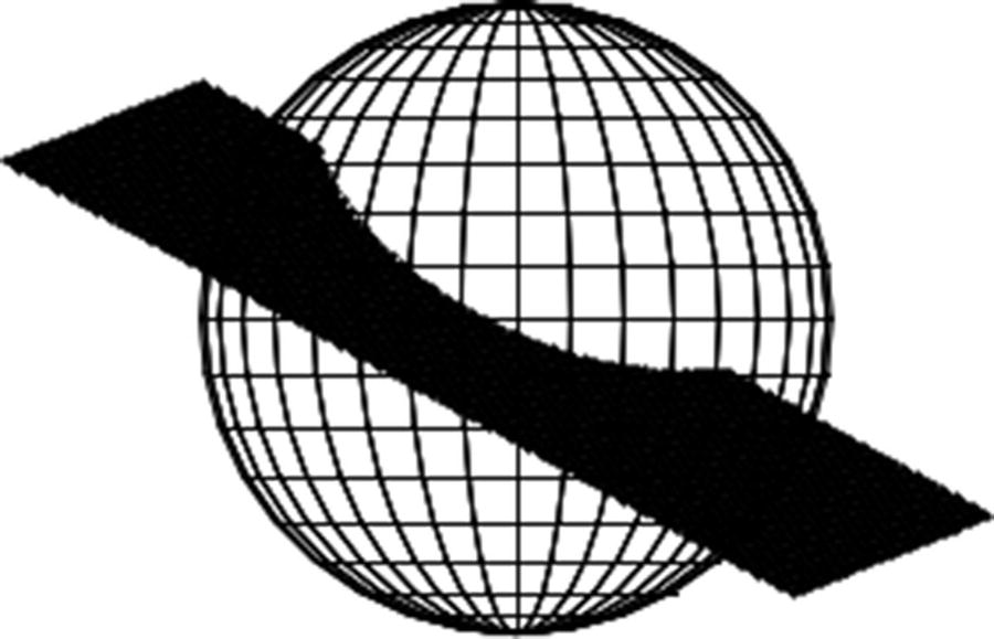
Plane intersecting a sphere produced by Listing 5-6

../images/456962_1_En_5_Chapter/456962_1_En_5_Fig24_HTML.jpg
Figure 5-24

Model for Listing 5-6

"""
PS
"""
import numpy as np
import matplotlib.pyplot as plt
from math import sin, cos, radians, sqrt
.
(similar to Program LS)
.
    #===================================================plane
1   def plane(xb,yb,zb,xe,ye,ze,Q12,dt):
2        hit='off'
3        for t in np.arange(0,Q12,dt): #———B to hit
4             xp=xb+ux*t
5             yp=yb+uy*t
6             zp=zb+uz*t
7             xpg=xc+xp
8             ypg=yc+yp
9             zpg=zc+zp
10            Qpc=sqrt(xp*xp+yp*yp+zp*zp)
11            if Qpc>=rs:
12                 plt.scatter(xpg,ypg,s=.5,color='k')
13            if Qpc<=rs:
14                 if hit=='off':
15                       hit='on'
16            if Qpc<rs:
17                 if hit=='on':
18                       plt.scatter(xpg,ypg,s=10,color=")
19            if Qpc>=rs:
20                 if hit=='on':
21                      hit='off'
22            if Qpc>rs:
23                 if hit=='off':
24                      plt.scatter(xpg,ypg,s=.5,color='k')
25
26  #———————————————————scan  across  plane
27  x1=-40
28  y1=-30
29  z1=-20
30
31  x2=60
32  y2=25
33  z2=-35
34
35  x3=-65
36  y3=-20
37  z3=-50
38
39  a=x2-x1
40  b=y2-y1
41  c=z2-z1
42  Q12=sqrt(a*a+b*b+c*c)
43  ux=a/Q12
44  uy=b/Q12
45  uz=c/Q12
46
47  a=x3-x1
48  b=y3-y1
49  c=z3-z1
50  Q13=sqrt(a*a+b*b+c*c)
51  vx=a/Q13
52  vy=b/Q13
53  vz=c/Q13
54
55  dt=.7 #————————————scan increment
56  ds=.7
57  for s in np.arange(0,Q13,ds):
58       sbx=x1+s*vx
59       sby=y1+s*vy
60       sbz=z1+s*vz
61       sex=x2+s*vx
62       sey=y2+s*vy
63       sez=z2+s*vz
64       plane(sbx,sby,sbz,sex,sey,sez,Q12,dt)
65
66  plt.axis([0,150,100,0]) #–replot axes and grid
67  plt.axis('off')
68  plt.grid(False)
69
70  plt.show() #–plot latest rotation
Listing 5-6

Program PS

5.7 Summary

In this chapter, you learned how to predict whether a three-dimensional line or plane will intersect a three-dimensional surface or solid object. Why bother with this? Because it is fundamental to removing hidden lines, you will see in Chapter 6. When plotting surface A, which may be behind another surface or object B, you do so in small steps, plotting a scatter dot (or a short line segment) at each step. If the point on A is hidden by B, you do not plot it. To determine if it is hidden from view by an observer, you draw an imaginary line from the point on A to the observer (i.e. in the -z direction). If you can determine if that line from A intersects a surface or object B in front of it, then you will know whether or not it is hidden. While you cannot develop hidden line algorithms for every conceivable situation (you did rectangular planes, triangular planes, circular sectors, circles, and spheres here), by understanding how it is done for these objects you should, with a bit of creativity, be able to develop your own hidden line algorithms for other surfaces and objects. Perhaps the line-triangular plane is most useful since complex surfaces and objects can often by approximated by an assembly of triangles. You will see more about this in Chapter 6.

..................Content has been hidden....................

You can't read the all page of ebook, please click here login for view all page.
Reset
18.117.183.172