Pandas is a remarkable tool for data analysis that aims to be the most powerful and flexible open source data analysis/manipulation tool available in any language. And, as you will soon see, if it doesn't already live up to this claim, it can't be too far off. Let's now take a look:

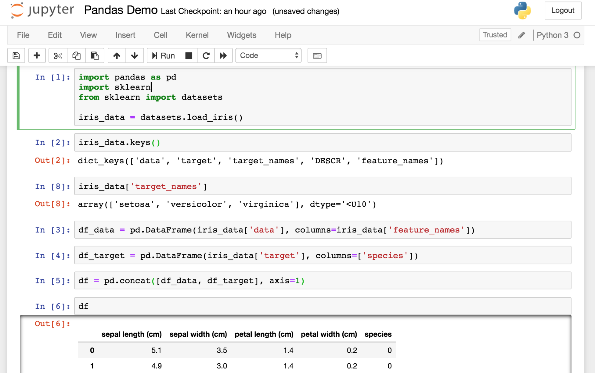
You can see from the preceding screenshot that I have imported a classic machine learning dataset, the iris dataset (also available at https://archive.ics.uci.edu/ml/datasets/Iris), using scikit-learn, a library we'll examine in detail later. I then passed the data into a pandas DataFrame, making sure to assign the column headers. One DataFrame contains flower measurement data, and the other DataFrame contains a number that represents the iris species. This is coded 0, 1, and 2 for setosa, versicolor, and virginica respectively. I then concatenated the two DataFrames.

For working with datasets that will fit on a single machine, pandas is the ultimate tool; you can think of it a bit like Excel on steroids. And, like the popular spreadsheet program, the basic units of operation are columns and rows of data that form tables. In the terminology of pandas, columns of data are series and the table is a DataFrame.

Using the same iris DataFrame we loaded previously, let's now take a look at a few common operations, including the following:

The first action was just to use the .head() command to get the first five rows. The second command was to select a single column from the DataFrame by referencing it by its column name. Another way we perform this data slicing is to use the .iloc[row,column] or .loc[row,column] notation. The former slices data using a numeric index for the columns and rows (positional indexing), while the latter uses a numeric index for the rows, but allows for using named columns (label-based indexing).

Let's select the first two columns and the first four rows using the .iloc notation. We'll then look at the .loc notation:

Using the .iloc notation and the Python list slicing syntax, we were able to select a slice of this DataFrame.

Now, let's try something more advanced. We'll use a list iterator to select just the width feature columns:

What we have done here is create a list that is a subset of all columns. df.columns returns a list of all columns, and our iteration uses a conditional statement to select only those with width in the title. Obviously, in this situation, we could have just as easily typed out the columns we wanted into a list, but this gives you a sense of the power available when dealing with much larger datasets.

We've seen how to select slices based on their position within the DataFrame, but let's now look at another method to select data. This time, we will select a subset of the data based upon satisfying conditions that we specify:

1. Let's now see the unique list of species available, and select just one of those:

2. In the far-right column, you will notice that our DataFrame only contains data for the Iris-virginica species (represented by the 2) now. In fact, the size of the DataFrame is now 50 rows, down from the original 150 rows:

3. You can also see that the index on the left retains the original row numbers. If we wanted to save just this data, we could save it as a new DataFrame, and reset the index as shown in the following diagram:

4. We have selected data by placing a condition on one column; let's now add more conditions. We'll go back to our original DataFrame and add two conditions:

The DataFrame now only includes data from the virginica species with a petal width greater than 2.2.

Let's now move on to using pandas to get some quick descriptive statistics from our iris dataset:

With a call to the .describe() function, I have received a breakdown of the descriptive statistics for each of the relevant columns. (Notice that species was automatically removed as it is not relevant for this.) I could also pass in my own percentiles if I wanted more granular information:

Next, let's check whether there is any correlation between these features. That can be done by calling .corr() on our DataFrame:

The default returns the Pearson correlation coefficient for each row-column pair. This can be switched to Kendall's Tau or Spearman's rank correlation coefficient by passing in a method argument (for example, .corr(method="spearman") or .corr(method="kendall")).