The Wolfram Language and Mathematica are exclusive tools and libraries of the Raspbian OS on the Raspberry Pi board. In this chapter, we explore the Wolfram Language and Mathematica from a programming view.
The following is a list of topics covered in this chapter:
Understand the Wolfram Language and Mathematica
Set up Wolfram and Mathematica
Develop a Hello World program
Learn basic programming for Wolfram and Mathematica
Learn computational mathematics with Wolfram and Mathematica
4.1 Introducing Wolfram Language and Mathematica
Wolfram Language and Mathematica are available for the Raspberry Pi board and come bundled with the Raspbian operating system. Programs can be run from a Pi command line or as a background process, as well as through a notebook interface on the Pi or on a remote computer. On the Pi, the Wolfram Language supports direct programmatic access to standard Pi ports and devices. For further information about this project, you can visit http://www.wolfram.com/raspberry-pi/.
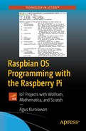
After you have deployed Raspbian on Raspberry Pi, you can run Raspbian in GUI mode and then you should see the Wolfram and Mathematica icons. You can see these icons in Figure 4-1.
Figure 4-1
The Wolfram and Mathematica icons on the Raspbian bar
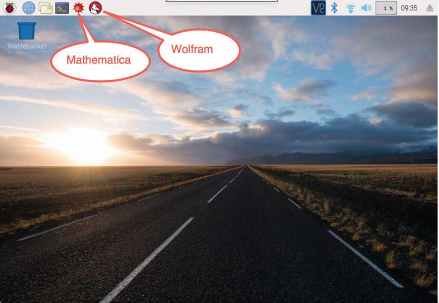
You also find these application icons in the main menu, as shown in Figure 4-2.
Figure 4-2
The Wolfram and Mathematica menu options on the Raspbian main menu
The Wolfram application has a Terminal form to run programs. If you execute the Wolfram application, you should see the Terminal application, as shown in Figure 4-3.
Figure 4-3
Running the Wolfram application from the Terminal
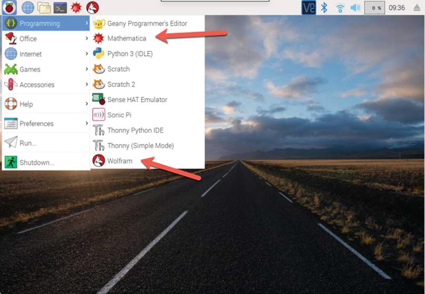
Otherwise, you can execute the Mathematica application. Then, you get the form shown in Figure 4-4.
Figure 4-4
Running the Mathematica application
Next, we learn how these tools work with computation mathematics.
4.2 Setting Up Wolfram and Mathematica
Technically, we don’t discuss setting up Wolfram and Mathematica in any more detail. If you download and deploy the latest Raspbian on the Raspberry Pi boards, you will get free licenses for Wolfram and Mathematica.
In the next section, we create a simple program on Wolfram and Mathematica.
4.3 Developing a Hello World Program
To get experience creating programs using Wolfram and Mathematica, we will build a simple program, using a simple mathematics operation. For demo purposes, you can click the Wolfram Mathematica icon. Then, you get the Wolfram Mathematica Editor, shown in Figure 4-5.
Now type these scripts:
a = 3
b = 5
c = a * b
Figure 4-5
Running programs on Mathematica
To run these scripts, press Shift+Enter (press the Shift and Enter keys together) and you’ll obtain the resulting output. Sample output can be seen in Figure 4-5.
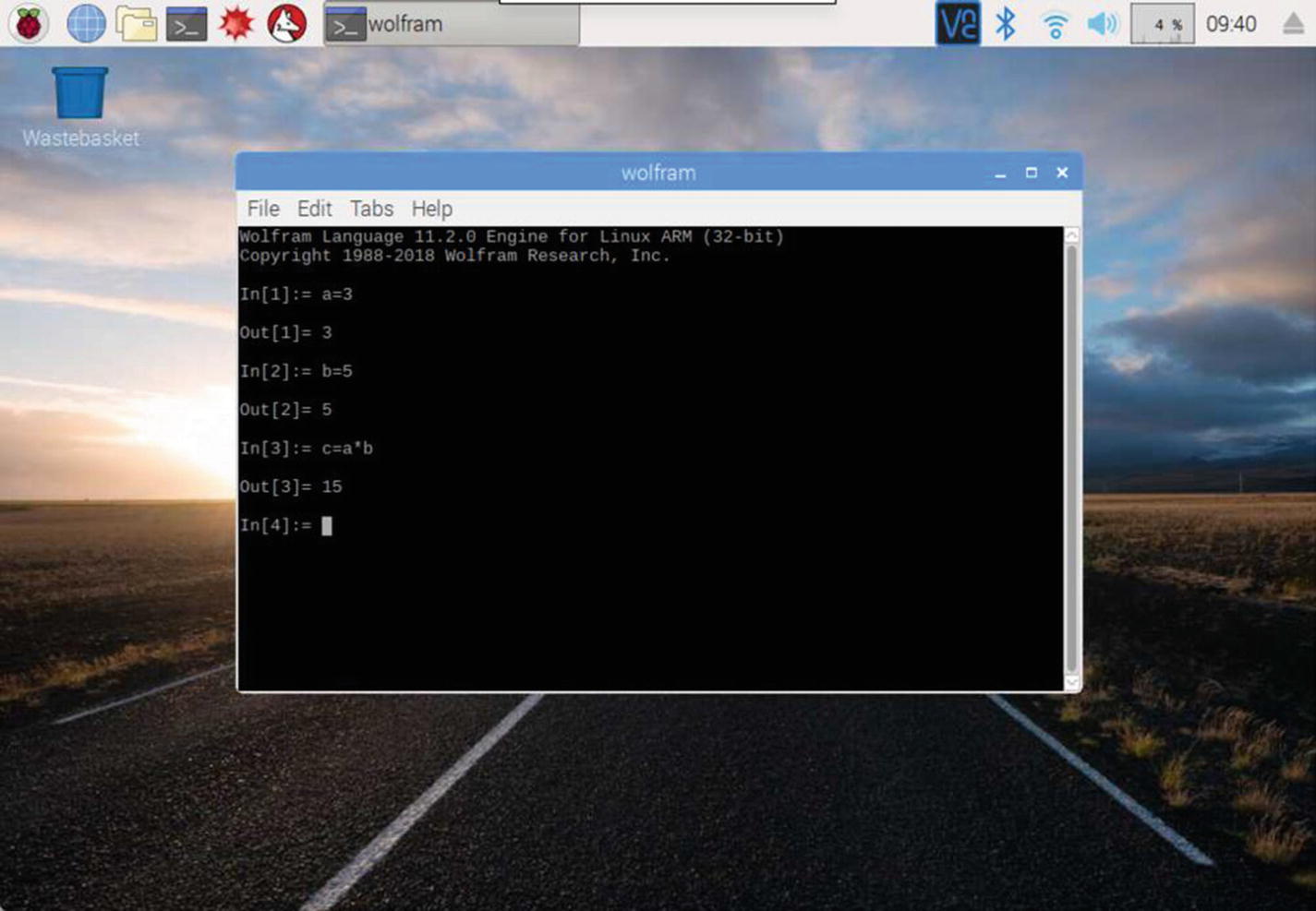
You also can run the same scripts in the Wolfram Terminal. You can type the script line-by-line. Then, you will get response directly. Sample program output from the Wolfram Terminal can be seen in Figure 4-6.
Figure 4-6
Running programs from the Wolfram Terminal
4.4 Basic Programming
In this section, you learn how to write programs for Wolfram and the Mathematica language. You learn the essential programming language steps from Wolfram and Mathematica.
You can follow the guidelines in the next sections.
4.4.1 Data Types and Declaring Variables
You can declare a variable and assign a value using the = syntax. If you don’t want to assign a value to a variable, you can set . as the value. You also can use := to delay assignment.
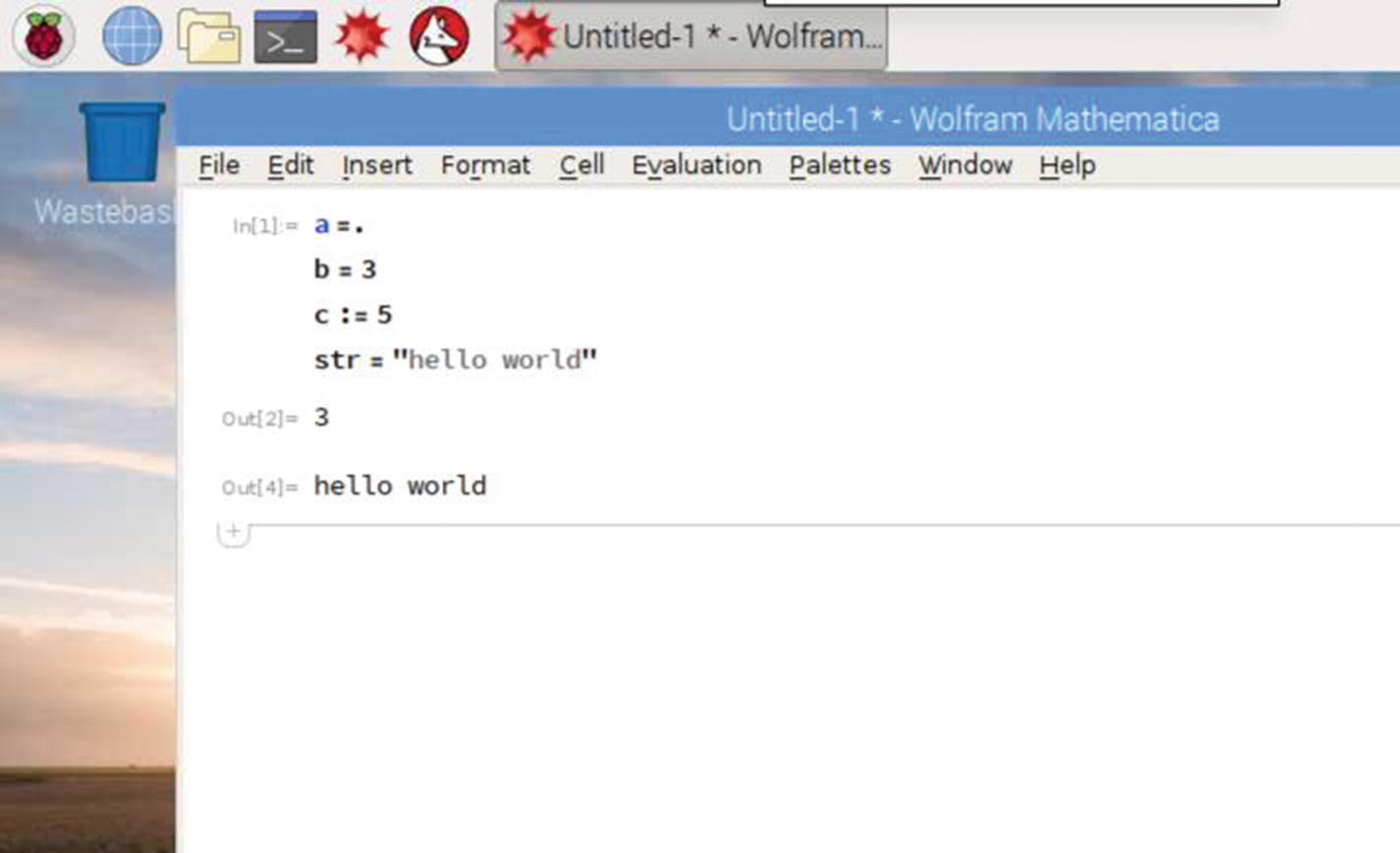
On a notebook from the Mathematica Editor, you can type these scripts:
a =.
b = 3
c := 5
str = "hello world"
Run these scripts by pressing the Shift+Enter keys. You can see the program output in Figure 4-7.
Figure 4-7
Declaring variables
4.4.2 Arithmetic Operators
Mathematica has arithmetic operators that you can use to manipulate numbers. The following is a list of its arithmetic operators:
Sometimes we want to manipulate data with a conditional. In Mathematica, we can use the if and switch statements. We explore these statements in the next sections.
4.4.4.1 if
We can write a Mathematica script for conditional statements, using the If[] statement. The following is general statement of if[].
If[statement,do if true, do if false]
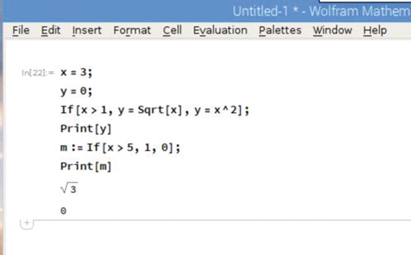
Let’s write this example:
x = 3;
y = 0;
If[x > 1, y = Sqrt[x], y = x^2];
Print[y]
m := If[x > 5, 1, 0];
Print[m]
You can type this program into Mathematica and you will get the program output shown in Figure 4-10.
Figure 4-10
Program output from an if application
4.4.4.2 switch
You can select one of several options in Mathematica. You can use the Switch[] statement. Switch[] can be defined as follows:
Switch[statement, case 1, do case 1 ...., case n,do case n, _ , do default case]
A sample Switch[] script can be written as follows:
k = 2;
n = 0;
Switch[k, 1, n = k + 10, 2, n = k^2 + 3, _, n = -1];
Print[n]
k = 5;
n := Switch[k, 1, k + 10, 2, k^2 + 3, _, -1];
Print[n]
Note
Print[] is used to print a message on the Terminal.
Run the program. You will get the program output that is shown in Figure 4-11.
Figure 4-11
Program output sample for Switch[]
4.4.5 Looping
If you perform continuous tasks, it’s wise to use a looping scenario to get those tasks done. In Mathematica, you can perform looping using the following statements:
do statements
for statements
while statements
Each type of looping statement will be reviewed in the next sections.
4.4.5.1 Do
The first looping statement is the Do[] statement. The Do[] statement can be defined as follows:
Do[do_something, {index}]
index is the amount of looping.
For instance, if you want to print “Hello Mathematica” five times, you would write this script.
Do[Print["Hello Mathematica"], {5}]
Run the program in Mathematica. If you do so, you’ll get the response shown in Figure 4-12.
Figure 4-12
Program output for a do statement
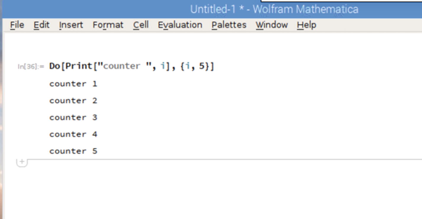
You also can include an index number in the looping statement. You can write this script for example:
Do[Print["counter ", i], {i, 5}]
After it’s executed, you’ll see the output shown in Figure 4-13.
Figure 4-13
Displaying an index on a looping program
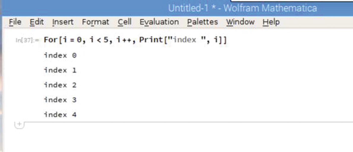
4.4.5.2 For
If you have experience with C/C++, you can use a for statement in the same way. The For[] statement in Mathematica is defined as follows:
For testing purposes, you can print a message five times. Write this script.
For[i = 0, i < 5, i++, Print["index ", i]]
Run the script and you’ll see the program output shown in Figure 4-14.
Figure 4-14
A looping program with For[]
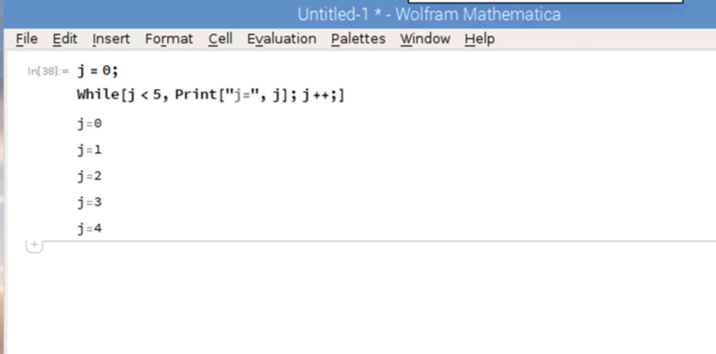
4.4.5.3 While
The last looping statement that we can use in Mathematica is While[]. This statement can be defined as follows:
While[conditional, do_something]
For demo purposes, write this script:
j = 0;
While[j < 5, Print["j=", j]; j++;]
This will print value 0 through value 4. You can see the program output in Figure 4-15.
Figure 4-15
Looping program written with While[]
4.4.5.4 Break and Continue
Break[] is used to exit the nearest enclosing loop. Continue[] is used to go to the next step in the current loop. Try writing these scripts for demo purposes:
For[i = 0, i < 10, i++,
Print[i];
If[i == 2, Continue[]];
If[i == 5, Break[]]
]
The program will stop a moment when the value of i is 2. The program also stops on value i = 5. You can see the program output in Figure 4-16.
Figure 4-16
Program demo using Break[] and Continue[]
4.4.6 Adding Comments
To add comments to your code, which is a very good idea, you can use the (* *) characters. You should use comments in your scripts, which the application will not run, to explain what certain lines of code and scripts are meant to do. Figure 4-17 shows comments added to scripts.
Figure 4-17
Adding comments to scripts
4.4.7 Functions
If you have scripts that are called continuously, consider using functions to avoid redundant scripts. You can wrap them into a function. A function in Mathematica can be defined as follows:
function[params_] := do_something
For testing purposes, we define a simple Mathematics function as follows:
Clear[f, x, y];
f[x_] := (x - 2) * Sqrt[x];
Print[f[15]];
Print[f[8]];
You should get the program output shown in Figure 4-18 when you execute these scripts.
Figure 4-18
A function in Mathematica
In a function, you can define parameters as input. You can also add two parameters or more. For instance, you can write these scripts.
Clear[f, x, y];
f[x_, y_] := x^2 + y;
Print[f[5, 8]];
Print[f[2, 3]];
The program output of these scripts can be seen in Figure 4-19.
Figure 4-19
A function with parameters
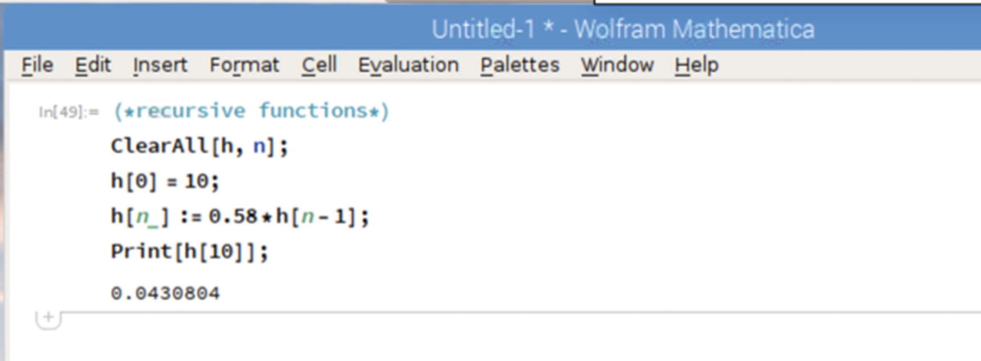
You can implement a recursive function in Mathematica as well. For instance, you can write these scripts:
(* recursive functions *)
ClearAll[h, n];
h[0] = 10;
h[n_] := 0.58 * h[n - 1];
Print[h[10]];
Now you can run this program. Figure 4-20 shows the program output sample.
Figure 4-20
A sample of a recursive function
4.5 Computational Mathematics
This chapter explains how to work with computational mathematics using Mathematica. We will discuss several mathematics problems as follows:
Calculus
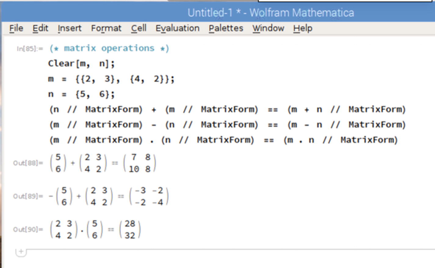
Matrix
Quadratic equations
Linear equations
Let’s go.
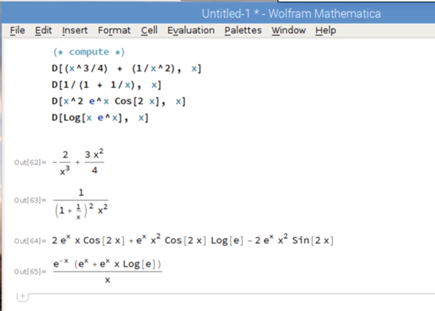
4.5.1 Calculus
There are many topics in calculus. In this section, we focus on plotting an equation, defining limits, performing differentiation, performing integration, and summing.
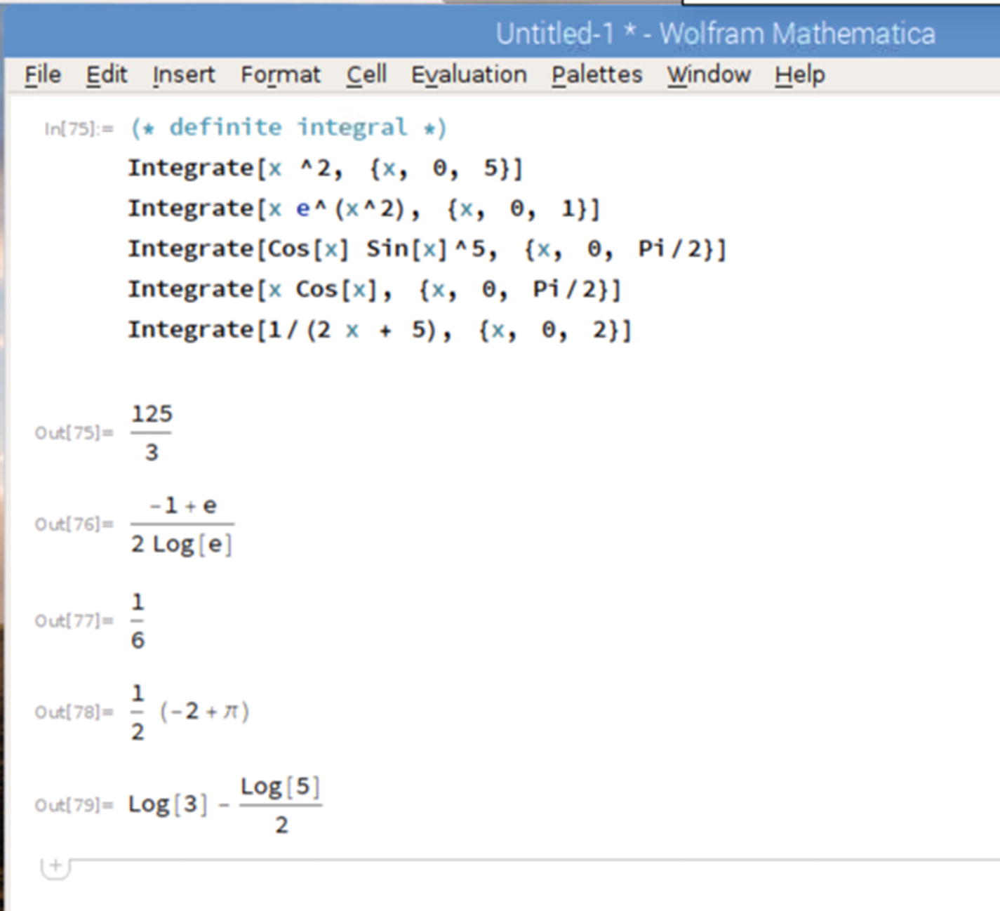
To implement a definite integral, you set the starting and ending values of the Integrate[] statement. Consider the following definite integral problems, for example.
You can solve those problems in Mathematica as follows.
In mathematics, there are many math problems related to summation. You can use Sum[] to calculate sums. For further information about Sum[], you can visit https://reference.wolfram.com/language/ref/Sum.html.
For instance, we have a formula as follows.
You can calculate that problem using Mathematica. Write scripts in Mathematica as follows.
Let’s look at some other examples. The following are quadratic equation problems. Find the x values.
Those problems can be solved in Mathematica. You can write these scripts to solve for x.
Solve[x^2 - 4 == 0, x]
Solve[6 x^2 + 11 x - 35 == 0, x]
Solve[x^2 - 7 x == 0, x]
The program output from Mathematica can be seen in Figure 4-37.
Figure 4-37
Quadratic equation solutions in Mathematica
4.5.4 Linear Equations
In linear equations, we solve to find values from a set of parameters. We can use the Solve[] statement in Mathematica to do this. For more information about this statement, visit https://reference.wolfram.com/language/ref/Solve.html.
For instance, we have three equations:
We can find the x, y, and z values in Mathematica.
Solve[{x + y + z, x + 2 y + 3 z, x - y + z} == {0, 1, 2}]
Another problem you can solve is as follows.
The solutions from these problems in Mathematica are as follows.
Solve[{3 x - y, y + 2 z, x + y + z} == {0, 1, 3}]
Run all these scripts. You’ll see the program output in Figure 4-38.
Figure 4-38
Solving linear equations using Mathematica
You can see the x, y, and z values.
Now we have another problem. The w parameter shown here is a constant value.
The solutions are written in Mathematica, as shown in the following script.
Solve[{2 x + 3 y - 7 z + w, 4 x - 2 y + z + 2 w, 5 x + y - 4 z + 3 w} == {8, 4, 6}]
In this chapter, you learned about the Wolfram and Mathematica programs in Raspbian OS that run on Raspberry Pi boards. You also played math games such as computational mathematics to see how to work with Mathematica.
In the next chapter, we focus on visual programming using Scratch on the Raspbian OS and Raspberry Pi boards.