
Chapter 2. A 3D/Math Primer
This chapter is an introduction to the mathematics behind 3D graphics. And in the immortal words of Douglas Adams (of Hitchhiker’s Guide to the Galaxy), “DON’T PANIC!” We discuss vectors, matrices, coordinate systems, transformations, and the DirectX Math library. Even if linear algebra is old hat to you, we encourage you to review the material specific to DirectX. Otherwise, take a deep breath, hold on, and don’t forget your towel.
Vectors
You might recall the definitions of scalars and vectors from your high school physics class. Scalars are quantities with just a magnitude (a numerical value); vectors are quantities described by both magnitude and direction. Vectors wear multiple hats in 3D graphics—they describe velocities, forces, directions, or simply positions in 3D space.
Geometrically, you can designate a vector as an arrow; the vector’s magnitude is its length and the line segment points along the direction of the vector. Under this definition, the tail of a vector has no fixed location. Thus, two vectors are equal if merely their lengths and their directions are the same. However, if you fix the tail at the origin of a coordinate system, the vector can describe a position specified by the number of components matching the dimensions of the coordinate system. In 3D space, you describe a vector by x, y, and z components. A position of (2, 5, 8) describes a vector whose head is located 2 units from the origin along the x-axis, 5 units along the y-axis, and 8 units along the z-axis. Figure 2.1 illustrates these concepts in 2D.
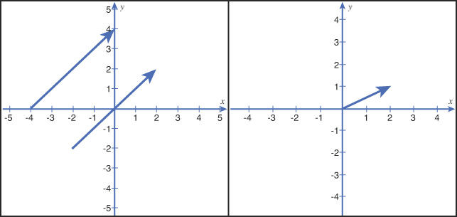
Figure 2.1 An illustration of vectors. To the left, the two vectors are equivalent, although their tails are drawn at different locations. To the right, a vector is rooted at the origin of a 2D coordinate system and describes a position.
Left-Handed and Right-Handed Coordinate Systems
The illustration in Figure 2.1 shows a 2D Cartesian coordinate system, where the x-axis runs horizontally and the y-axis runs vertically, with positive numbers to the right and up, respectively. In 3D space, the z-axis is orthogonal (perpendicular) to the x- and y-axes, with positive numbers running into or out of the screen, depending on the handedness of the coordinate system. In a left-handed coordinate system, positive z-values move into the screen, and they move out of the screen for a right-handed system. A useful mnemonic for handedness is to hold your right hand in front of you, pointing your thumb toward the positive x-axis and your index finger toward the positive y-axis. The direction of your middle finger (toward you) indicates the positive z-values headed out of the screen; conversely, the opposite is true for your left hand. Figure 2.2 illustrates this technique.
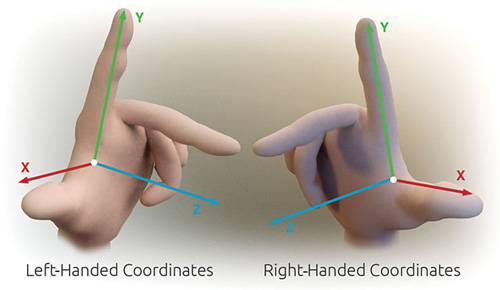
Figure 2.2 A mnemonic for 3D coordinate system handedness. (By Primalshell [CC-BY-SA-3.0 (http://creativecommons.org/licenses/by-sa/3.0)] via Wikimedia Commons.)
Basic Vector Operations
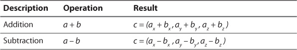
Two vectors are added and subtracted component wise—that is, the operands are drawn from matching components of the two vectors. For example, if you define two vectors a = (ax, ay, az) and b = (bx, by, bz), and perform addition or subtraction between them to produce vector c, then these operations are performed according to Table 2.1.
Likewise, multiplication and division are performed component wise as are basic operations between a scalar and a vector. The following is an example of scalar multiplication:
4 * a = (4ax, 4ay, 4az)
Vector Length
The length (or magnitude) of a vector is calculated using the Pythagorean Theorem. Specifically, you use the following equation (for a three-dimensional vector):
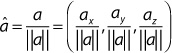
A vector whose length is exactly 1 is called a unit vector. Such vectors are useful for situations that require only the direction of the vector, not its magnitude. When you force a vector to have a length of 1, it’s called normalizing the vector; it is accomplished by dividing the vector by its magnitude. In equation form:
Dot Product
The dot product between two vectors is the sum of the products of the matching components. In equation form:
a • b = (ax * bx) + (ay * by) + (az * bz)
This produces a scalar value, hence the dot product is also referred to as the scalar product (or inner product). Considering the definition of vector length, you can use the square root of the vector dotted with itself to compute the vector’s magnitude.
Geometrically, the dot product describes an angle between two vectors. In equation form:
a • b = ||a||*||b|| * cos(θ)
Where θ is the angle between vectors a and b. If both vectors are unit length, the dot product reduces to:
a • b = cos(θ)
From this equation, you can observe the following:
![]() If a • b > 0, then the angle between the vectors is less than 90 degrees.
If a • b > 0, then the angle between the vectors is less than 90 degrees.
![]() If a • b < 0, then the angle between the vectors is greater than 90 degrees.
If a • b < 0, then the angle between the vectors is greater than 90 degrees.
![]() If a • b = 0, then the vectors are orthogonal.
If a • b = 0, then the vectors are orthogonal.
As you’ll see in coming chapters, the dot product has a variety of applications in computer graphics. For instance, the dot product is useful in lighting calculations to determine the angle between the surface and a light source. We discuss such applications in detail in Part II, “Shader Authoring with HLSL.”
Cross Product
Another useful vector operation is the cross product. The cross product of two vectors produces a third vector that is orthogonal to the two other vectors. The equation for cross product is:
a × b = (ay * bz – az * by, az * bx – ax * bz, ax * by – ay * bx)
You can use the cross product, for example, to compute the surface normal of a triangle (which describes the direction the triangle faces).
Matrices
An m×n matrix is a two-dimensional array of numbers with m rows and n columns. A 4×1 matrix, for example, has four rows and one column. A 2×3 matrix has two rows and three columns. Such matrices are notated as follows:
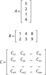
Note the matrix C, which depicts the subscript notation for identifying an element within the matrix.
Matrices with only a single row or column are sometimes referred to as row vectors or column vectors. Matrices with the same number of rows and columns are known as square matrices. In 3D graphics, 4×4 square matrices are used extensively.
Basic Matrix Operations
You can perform a number of basic arithmetic operations on matrices. As with vectors, addition and subtraction are performed component wise. Thus, the two matrices must have the same number of rows and columns. Scalar multiplication is also performed component wise, with the scalar multiplied with each element of the matrix. However, matrix-to-matrix multiplication is a bit different.
Matrix Multiplication
For matrix multiplication, a matrix with n columns can be multiplied only by a matrix with n rows. Each element in the resulting matrix is computed as the dot product between the rows in the first matrix and the corresponding columns in the second matrix. In equation form, if you consider each row of matrix A as a row vector and each column of matrix B as a column vector, you can define the elements of the product C as follows:
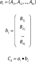
Figure 2.3 illustrates this process.
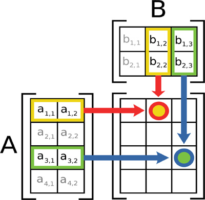
Figure 2.3 Matrix multiplication. (By Bilou [GFDL (http://www.gnu.org/copyleft/fdl.html), CC-BY-SA-3.0 (http://creativecommons.org/licenses/by-sa/3.0/)], via Wikimedia Commons.)
By way of example, consider the following matrices:
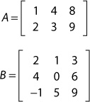
Matrix A has two rows and three columns (a 2×3 matrix). Matrix B has three rows and three columns (a 3×3 matrix). The number of rows in B is equal to the number of columns in A, so multiplication is permitted. The resulting product is a 2×3 matrix and is computed as:

Note that matrix multiplication is not commutative (you can’t reverse the operands and yield the same value). Indeed, it’s common that multiplication defined for A * B is undefined for B * A, as is the case for a 3×3 matrix multiplied by a 2×3 matrix.
Transposition
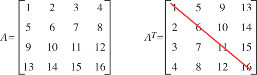
The transpose of a matrix is found by reflecting its elements over its main diagonal. For a square matrix, this is easy to envision, as the following example demonstrates:
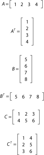
Another way to think of transposing a matrix is swapping the rows and columns. This approach might be simpler to imagine, particularly for row vectors and column vectors, or nonsquare matrices. For example:
Row-Major and Column-Major Order
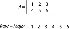
When dealing with matrices, you must consider how they are stored in a computer’s memory. Direct3D stores matrices in row-major order—that is, if stored in contiguous memory, the rows are laid out one after another. This is also the format of multidimensional arrays in the C programming language. The following example shows a 2×3 matrix stored contiguously in row-major order.
Conversely, the same matrix, written in column-major order, would appear in memory as:
Column − Major: 1 4 2 5 3 6
Converting a row-major matrix to a column-major matrix (or vice versa) involves transposing it. How a matrix is stored in memory can have performance implications, and various library methods depend on a particular order. We discuss this further in Chapter 4, “Hello, Shaders!”
The Identity Matrix
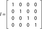
The identity matrix is a special square matrix that has ones along the main diagonal and zeroes everywhere else. For example, a 4×4 identity matrix is defined as:
The identity matrix is essentially the number one, with respect to matrix multiplication. In other words, multiplying a matrix by the identity matrix results in the original matrix.
Transformations
As mentioned previously, vectors describe (among other things) directions and positions in 3D space. For instance, the positions of the vertices of your 3D triangles are stored in vectors, as are their surface normals. However, these vectors are unlikely to remain static throughout their lives inside your graphics applications. Your 3D objects will move, grow, shrink, and turn within a scene. More formally, displacement is known as translation, growing and shrinking is scaling, and turning is rotation. Such operations are known as transformations. Furthermore, to display your objects to the screen, they will be considered from multiple frames of reference—coordinate systems. You’ll use matrices to transform positions and directions from one coordinate system to another, as well as to apply translation, scaling, and rotation.
Homogeneous Coordinates
Before diving into the specific transformation matrices, it’s important to note that we’ll be using homogeneous coordinates. This coordinate system enables you to incorporate translation into a 4×4 matrix along with scaling and rotation. Matrix multiplication is associative, so a single 4×4 matrix can encapsulate all these transformations. With homogeneous coordinates, each position has four components: x, y, z, and w. The xyz coordinates are the normal 3D coordinates, and the w component is the value 1 for positions and 0 for directions. As you’ll see, the w = 0 for direction vectors nullifies translation, which makes sense because direction vectors have no location in 3D space.
Scaling
To transform a vector, you perform a vector-to-matrix multiplication, which is just a matrix multiplication against a row vector or column vector. By way of example, the 3D scaling matrix is defined as:
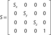
The values along the main diagonal represent the scaling factors for the x-, y-, and z-axes. If these values are the same, the vector will be scaled uniformly. Note the similarity to the identity matrix, which is merely a scaling matrix with ones along the diagonal.
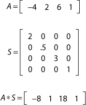
Following is an example of transforming a position vector by a nonuniform scaling matrix. The position stored in A is (–4, 2, 6). The fourth column (the w component with the value 1) is necessary because the scaling matrix has four rows.
Translation
The act of translation moves an object along the x-, y-, and z-axes. The translation matrix is defined as:

Next is an example of translating a position vector 10 units along the x-axis, 5 units along the y-axis, and 6 units along the negative z-axis.
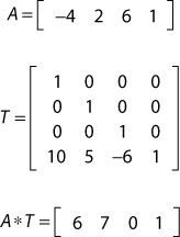
Notice that if the w component of the vector was 0 (as if the vector represented a direction), the transformation would have no impact.
Rotation
Rotation is a bit more complicated because each axis has a different rotation matrix.
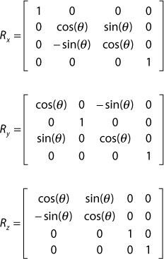
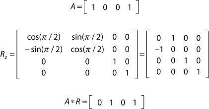
Following is an example of rotating the position (1, 0, 0) 90 degrees (π/2 radians) counterclockwise around the z-axis.
Matrix Concatenation
Instead of applying each of these transforms individually, they can be concatenated into a single transformation matrix. For example, a scale, rotation, and translation matrix can be combined as:
W = S * R * T
Transforming a position vector by this concatenated matrix scales, rotates, and translates the vector in a single operation. However, the order of concatenation is important. Concatenation is performed from left to right, and matrix multiplication is not commutative. For example, suppose you were rendering Earth orbiting the sun. It has both a translation away from the sun and a rotation around it, and the concatenation should be performed in that order. However, if you also wanted to simulate Earth’s axial rotation, you’d want to perform that rotation before the “orbit” transformations. In such a scenario, the complete concatenated matrix would appear as:
W = Raxial * T * Rorbit
You can concatenate any number of individual transforms; just be aware of the left-to-right ordering.
Changing Coordinate Systems
In addition to scaling, translation, and rotation, you can use transformation matrices to move a vector from one coordinate system to another.
Object Space and World Space
Typically, you will create your 3D models in a digital content creation package, such as Autodesk Maya or 3D Studio Max. You also will author a model in its own coordinate system, called object space (or model space). Your scenes might contain hundreds of individual models, but these objects are rarely authored as a whole. Instead, each object is stored in a separate file, and its vertices are relative to its own origin, with no relationship to another 3D model. For these objects to interact, they must share a common coordinate system—they must exist in the same world. Therefore, they must be transformed from object space to world space.
A world transformation matrix (or world matrix) is made from concatenated scale, translation, and rotation matrices. To apply the world matrix to a 3D model is to multiply each vertex in the object by the matrix.
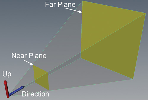
View Space
From world space, the object is then transformed into view space (or camera space), a coordinate system relative to a virtual camera. The properties of the camera define a volume within which objects are visible. This volume is known as the view frustum (see Figure 2.4). A view matrix is used to transform vectors from world space to view space and is commonly created through a combination of the camera’s position (in world space), a vector describing where the camera is looking, and a vector describing which way is “up.” You use the DirectX API to create a view matrix in Part III, “Rendering with DirectX.”
Projection Space
Object space, world space, and view space are all three-dimensional coordinate systems. However, computer screens are two-dimensional, and the projection matrix projects this 3D geometry onto a 2D display. In this stage, the illusion of depth is created—for example, objects that are closer to the screen appear larger than those farther away. This is known as perspective projection, as opposed to orthographic projection, in which all objects appear to be the same distance away from the camera, regardless of their actual positions.
The properties of the projection matrix help define the view frustum and include a near plane and far plane, a vertical field of view, and an aspect ratio. Objects between the camera’s position and the near plane are not rendered, nor are objects past the far plane. A good analogy is the tip of your nose (near plane) and the horizon (far plane). The field of view defines the extent of the frustum, and the aspect ratio is typically the width of the display (or window) divided by the height. As with the view matrix, the projection matrix is commonly constructed through DirectX API calls.
The transformations for world, view, and projection space are typically performed within the vertex shader, and you are responsible for them. You can apply each transformation individually, or you can concatenate the three matrices into what’s commonly referred to as the world-view-projection matrix, or WVP. After they’re multiplied by the projection matrix, the coordinates are in projection space (or homogeneous clip space).
DirectXMath
DirectXMath is a SIMD-friendly C++ API from Microsoft that supports the mathematics common to graphics applications. SIMD stands for Single Instruction Multiple Data and provides for multiple data points to be operated on through a single CPU instruction. For example, on the Windows platform, SIMD instructions can operate on four 32-bit floats simultaneously. This offers significant performance gains. For example, if you added two vectors together, each with four components, you would ordinarily perform four add instructions. But with SIMD, the same addition can be performed with a single instruction.
DirectXMath is distributed as part of the Windows SDK (we discuss this further in Chapter 3, “Tools of the Trade”). To use the library, simply include the DirectXMath.h file in your applications. All the implementation is included in the header file; it has no libraries to link against.
Vectors
Vectors are supported through XMVECTOR, a 16-byte aligned data type mapped to SIMD registers. For best performance, all vector operations (for example, addition or subtraction) should be performed through XMVECTOR instances. However, this is an opaque data type, so individual vector components are inaccessible as structure members. Additionally, because this data type is 16-byte aligned, it’s not a good candidate for class member storage. For class storage, the types XMFLOAT2, XMFLOAT3, and XMFLOAT4 are recommended instead. These types have accessible members for two, three, and four components (x, y, z, and w), respectively.
Loading and Storing
To take advantage of SIMD instructions, you need to copy data out of XMFLOAT* instances and into XMVECTOR objects. You accomplish this with the following load methods:
XMVECTOR XMLoadFloat2(const XMFLOAT2* pSource);
XMVECTOR XMLoadFloat3(const XMFLOAT3* pSource);
XMVECTOR XMLoadFloat4(const XMFLOAT4* pSource);
Conversely, you copy data out of XMVECTOR instances and into XMFLOAT* objects through the following store methods:
void XMStoreFloat2(XMFLOAT2* pDestination, FXMVECTOR V);
void XMStoreFloat3(XMFLOAT3* pDestination, FXMVECTOR V);
void XMStoreFloat4(XMFLOAT4* pDestination, FXMVECTOR V);
Thus, the pattern for using vectors in DirectXMath is to store XMFLOAT* instances as class members and load them into local XMVECTOR objects for SIMD vector operations. If you need to save the output of a vector operation, you store the resulting XMVECTOR object back into an XMFLOAT* class member.
Note
DirectXMath supports vectors with many other underlying data types, including byte, int, short, and half-float (16-bit floats). They all follow the same naming and calling conventions. For example, XMBYTE4 stores four 8-bit signed values and has matching load and store methods: XMLoadByte4() and XMStoreByte4().
Calling Conventions
Note the FXMVECTOR type in the parameter lists of the store functions. This is one of four aliases used for XMVECTOR—the others are GXMVECTOR, HXMVECTOR, and CXMVECTOR. These aliases are used for optimal data layout and portability between platforms. On the x86 and Xbox 360 platforms, these are simply synonyms for XMVECTOR. For the x64 platform, these types are XMVECTOR references. The rules for passing XMVECTOR arguments follow:
![]() Use
Use FXMVECTOR for the first three XMVECTOR input parameters.
![]() Use
Use GXMVECTOR for the fourth XMVECTOR input parameter.
![]() Use
Use HXMVECTOR for the fifth and sixth XMVECTOR input parameters.
![]() Use
Use CXMVECTOR for any additional XMVECTOR input parameters.
![]() Use
Use XMVECTOR* or XMVECTOR& for all output parameters.
You can find more details concerning DirectXMath calling conventions in the online documentation at http://msdn.microsoft.com/en-us/library/windows/desktop/hh437833(v=vs.85).aspx.
Accessors and Mutators
Although XMVECTOR objects are opaque, you need not store or load the object if you need to read or write only a single component. Instead, you can use the following accessor and mutator methods:
float XMVectorGetX(XMVECTOR V);
float XMVectorGetY(XMVECTOR V);
float XMVectorGetZ(XMVECTOR V);
float XMVectorGetW(XMVECTOR V);
void XMVectorSetX(XMVECTOR V, float X);
void XMVectorSetY(XMVECTOR V, float Y);
void XMVectorSetZ(XMVECTOR V, float Z);
void XMVectorSetW(XMVECTOR V, float W);
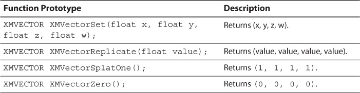
Initialization Functions
You can also initialize XMVECTOR objects in a variety of ways. Table 2.2 lists some common initialization functions.
Operators
XMVECTOR has a series of overloaded operators for vector-to-vector addition, subtraction, multiplication, and division, as well as scalar-to-vector multiplication. These operators are listed here:
XMVECTOR operator+ (FXMVECTOR V);
XMVECTOR operator- (FXMVECTOR V);
XMVECTOR& operator+= (XMVECTOR& V1, FXMVECTOR V2);
XMVECTOR& operator-= (XMVECTOR& V1, FXMVECTOR V2);
XMVECTOR& operator*= (XMVECTOR& V1, FXMVECTOR V2);
XMVECTOR& operator/= (XMVECTOR& V1, FXMVECTOR V2);
XMVECTOR& operator*= (XMVECTOR& V, float S);
XMVECTOR& operator/= (XMVECTOR& V, float S);
XMVECTOR operator+ (FXMVECTOR V1, FXMVECTOR V2);
XMVECTOR operator- (FXMVECTOR V1, FXMVECTOR V2);
XMVECTOR operator* (FXMVECTOR V1, FXMVECTOR V2);
XMVECTOR operator/ (FXMVECTOR V1, FXMVECTOR V2);
XMVECTOR operator* (FXMVECTOR V, float S);
XMVECTOR operator* (float S, FXMVECTOR V);
XMVECTOR operator/ (FXMVECTOR V, float S);
Vector Functions
DirectXMath has a variety of vector functions that support the operations discussed in this chapter. Table 2.3 lists commonly used functions for 3D vectors. Note that most of these functions also exist in 2D and 4D form.
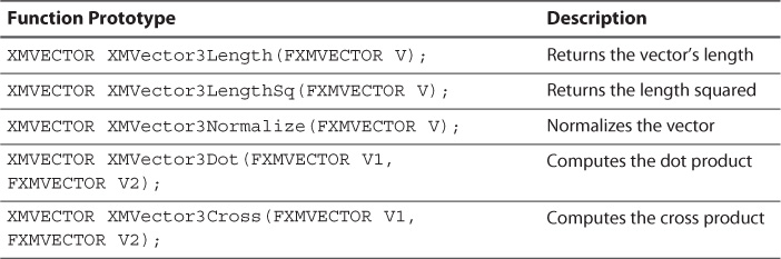
Note
For the vector functions in Table 2.3, the operations that return a scalar replicate the value across each of the XMVECTOR components.
Matrices
Matrices are supported through the XMMATRIX type—an array of four XMVECTOR objects. Just as with XMVECTOR, XMMATRIX objects aren’t good candidates for class storage. Types such as XMFLOAT3X3 and XMFLOAT4X4 should be used instead. XMFLOAT4X4 has the following structure:
struct XMFLOAT4X4
{
union
{
struct
{
float _11, _12, _13, _14;
float _21, _22, _23, _24;
float _31, _32, _33, _34;
float _41, _42, _43, _44;
};
float m[4][4];
};
Thus, you can access elements in traditional matrix subscript form or through zero-based [row, column] array access.
Loading and Storing
XMMATRIX objects have load and store functions similar to XMVECTOR objects. For example:
XMVECTOR XMLoadFloat4×4(const XMFLOAT4X4* pSource);
void XMStoreFloat4×4(XMFLOAT4X4* pDestination, FXMMATRIX M);
Notice the type FXMMATRIX in the store method. Similar to the vector object, this is one of two aliases for XMMATRIX; the other is CXMMATRIX. Essentially, the calling conventions for XMMATRIX are to use FXMMATRIX for the first argument and use CXMMATRIX for everything else. A few exceptions to this rule apply; see the online documentation for details.
Accessors, Mutators, and Initialization
XMMATRIX has an accessible member r for the array of XMVECTOR objects it contains. You can use it in conjunction with the XMVECTOR accessor, mutator, and initialization functions. An XMMATRIX can also be initialized through two constructors that accept either 4 XMVECTOR objects or 16 individual floats. In addition, you can initialize an identity matrix through this function:
XMMATRIX XMMatrixIdentity();
Operators
XMMATRIX has a set of overloaded operators for matrix-to-matrix addition, subtraction, and multiplication, as well as scalar-to-matrix multiplication and division. These operators are listed here:
XMMATRIX& operator+= (FXMMATRIX M);
XMMATRIX& operator-= (FXMMATRIX M);
XMMATRIX& operator*= (FXMMATRIX M);
XMMATRIX& operator*= (float S);
XMMATRIX& operator/= (float S);
XMMATRIX operator+ (FXMMATRIX M) const;
XMMATRIX operator- (FXMMATRIX M) const;
XMMATRIX operator* (FXMMATRIX M) const;
XMMATRIX operator* (float S) const;
XMMATRIX operator/ (float S) const;
Matrix Functions
DirectXMath includes a number of functions for performing matrix operations (such as the ones discussed in this chapter). Table 2.4 lists some of the more commonly used functions.
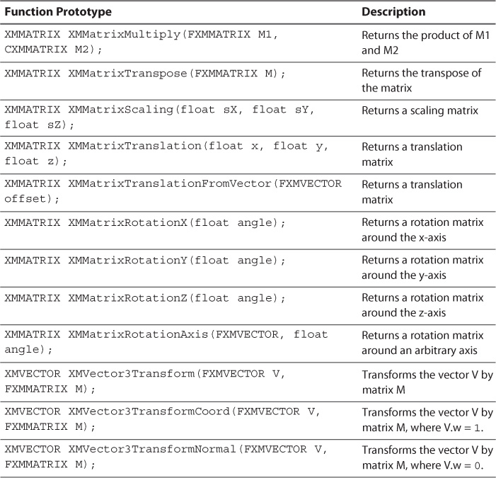
The last three functions in Table 2.4 perform vector-to-matrix multiplication using three-dimensional vectors. Note that you need not explicitly set the w component of the input vector for any of these functions. In XMVector3Transform() and XMVector3TransformCoord(), the value 1.0 is used for the w component. For XMVector3TransformNormal(), the fourth row (the translation row) is ignored. For XMVector3Transform(), the w component of the returned vector may be nonhomogeneous (not 1.0); for XMVector3TransformCoord(), the w component of the returned vector is guaranteed to be 1.0.
Summary
This chapter provided an introduction to the mathematics behind 3D graphics. You’ve learned about vectors, matrices, coordinate systems, and transformations, and you’ve seen some of their use in graphics programming. You’ve also discovered the DirectXMath library, a cross-platform, SIMD-friendly C++ API for graphics applications.
This introduction focused on concepts central to graphics programming, but it just scratched the surface of a much larger topic. Indeed, entire books are dedicated to graphics-related mathematics, to which we’ve devoted only this single chapter. Likewise, the DirectXMath library has much more functionality than we’ve covered here. If you are interested in exploring these subjects further, many printed and online resources are available.