2 Your first NLP application

This chapter covers

• Building a sentiment analyzer using AllenNLP
• Applying basic machine learning concepts (datasets, classification, and regression)
• Employing neural network concepts (word embeddings, recurrent neural networks, linear layers)
• Training the model through reducing loss
• Evaluating and deploying your model

In section 1.1.2, we saw how not to do NLP. In this chapter, we are going to discuss how to do NLP in a more principled, modern way. Specifically, we’d like to build a sentiment analyzer using a neural network. Even though the sentiment analyzer we are going to build is a simple application and the library (AllenNLP) takes care of most heavy lifting, it is a full-fledged NLP application that covers a lot of basic components of modern NLP and machine learning. I’ll introduce important terms and concepts along the way. Don’t worry if you don’t understand some concepts at first. We will revisit most of the concepts introduced here in later chapters.

2.1 Introducing sentiment analysis

In the scenario described in section 1.1.2, you wanted to extract users’ subjective opinions from online survey results. You have a collection of textual data in response to a free-response question, but you are missing the answers to the “How do you like our product?” question, which you’d like to recover from the text. This task is called sentiment analysis, which is a text analytic technique used in the automatic identification and categorization of subjective information within text. The technique is widely used in quantifying opinions, emotions, and so on that are written in an unstructured way and, thus, hard to quantify otherwise. Sentiment analysis is applied to a wide variety of textual resources such as survey, reviews, and social media posts.

In machine learning, classification means categorizing something into a set of predefined, discrete categories. One of the most basic tasks in sentiment analysis is the classification of polarity, that is, to classify whether the expressed opinion is positive, negative, or neutral. You could use more than three classes, for example, strongly positive, positive, neutral, negative, or strongly negative. This may sound familiar to you if you have used a website (such as Amazon) where people can review things using a five-point scale expressed by the number of stars.

Classification of polarity is one type of sentence classification task. Another type of sentence classification task is spam filtering, where each sentence is categorized into two classes—spam or not spam. It’s called binary classification if there are only two classes. If there are more than two classes (the five-star classification system mentioned earlier, for example), it’s called multiclass classification.

In contrast, when the prediction is a continuous value instead of discrete categories, it’s called regression. If you’d like to predict the price of a house based on its properties, such as its neighborhood, numbers of bedrooms and bathrooms, and square footage, it’s a regression problem. If you attempt to predict stock prices based on the information collected from news articles and social media posts, it’s also a regression problem. (Disclaimer: I’m not suggesting this is an appropriate approach to stock price prediction. I’m not even sure if it works.) As I mentioned earlier, most linguistic units such as characters, words, and part-of-speech tags are discrete. For this reason, most uses of machine learning in NLP are classification, not regression.

NOTE Logistic regression, a widely used statistical model, is usually used for classification, even though it has “regression” in its name. Yes, I know it’s confusing!

Many modern NLP applications, including the sentiment analyzer we are going to build in this chapter (shown in figure 2.1), are built based on the supervised machine learning paradigm. Supervised machine learning is one type of machine learning where the algorithm is trained with data that has supervision signals—the desired outcome for individual input. The algorithm is trained in such a way that it reproduces the signals as closely as possible. For sentiment analysis, this means that the system is trained on data that contains the desired labels for each input sentence.

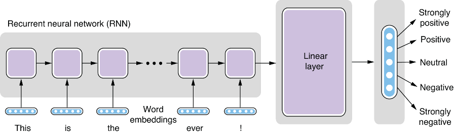
Figure 2.1 Sentiment analysis pipeline

2.2 Working with NLP datasets

As we discussed in the previous section, many modern NLP applications are developed using supervised machine learning, where algorithms are trained from data annotated with desired outcomes, instead of using handwritten rules. Almost by definition, data is a critical part for machine learning, and it is important to understand how it is structured and used with machine learning algorithms.

2.2.1 What is a dataset?

A dataset simply means a collection of data. If you are familiar with relational databases, you can think of a dataset as a dump of one table. It consists of pieces of data that follow the same format. In database terms, each piece of the data corresponds to a record, or a row in a table. A record can have any number of fields, which correspond to columns in a database.

In NLP, records in a dataset are usually some type of linguistic units, such as words, sentences, or documents. A dataset of natural language texts is called a corpus (plural: corpora). As an example, let’s think of a (hypothetical) dataset for spam filtering. Each record in this dataset is a pair of a piece of text and a label, where the text is a sentence or a paragraph (e.g., from an email) and the label specifies whether the text is spam. Both the text and the label are the fields of a record.

Some NLP datasets and corpora have more complex structures. For example, a dataset may contain a collection of sentences, where each sentence is annotated with detailed linguistic information, such as part-of-speech tags, parse trees, dependency structures, and semantic roles. If a dataset contains a collection of sentences annotated with their parse trees, the dataset is called a treebank. The most famous example of this is Penn Treebank (PTB) (http://realworldnlpbook.com/ch2.html#ptb), which has been serving as the de facto standard dataset for training and evaluating NLP tasks such as part-of-speech (POS) tagging and parsing.

A closely related term to a record is an instance. In machine learning, an instance is a basic unit for which the prediction is made. For example, in the spam-filtering task mentioned earlier, an instance is one piece of text, because predictions (spam or not spam) are made for individual texts. An instance is usually created from a record in a dataset, as is the case for the spam-filtering task, but this is not always the case—for example, if you take a treebank and use it to train an NLP task that detects all nouns in a sentence, then each word, not a sentence, becomes an instance, because prediction (noun or not noun) is made for each word. Finally, a label is a piece of information attached to some linguistic unit in a dataset. A spam-filtering dataset has labels that correspond to whether each text is a spam. A treebank may have one label per word for its part of speech. Labels are usually used as training signals (i.e., answers for the training algorithm) in a supervised machine learning setting. See figure 2.2 for a depiction of these parts of a dataset.

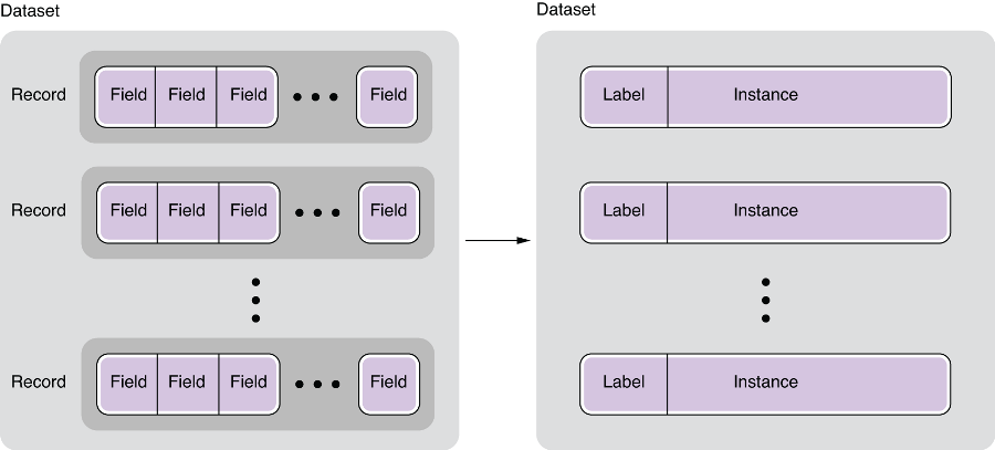
Figure 2.2 Datasets, records, fields, instances, and labels

2.2.2 Stanford Sentiment Treebank

To build a sentiment analyzer, we are going to use the Stanford Sentiment Treebank (SST; https://nlp.stanford.edu/sentiment/), one of the most widely used sentiment analysis datasets as of today. Go ahead and download the dataset from the Train, Dev, Test Splits in PTB Tree Format link. One feature that differentiates SST from other datasets is the fact that sentiment labels are assigned not only to sentences but also to every word and phrase in sentences. For example, some excerpts from the dataset follow:

(4
  (2 (2 Steven) (2 Spielberg))
    (4
      (2 (2 brings) (3 us))
      (4 (2 another) (4 masterpiece))))
 
(1
  (2 It)
  (1
    (1 (2 (2 's) (1 not))
      (4 (2 a) (4 (4 great) (2 (2 monster) (2 movie)))))
    (2 .)))

Don’t worry about the details for now—these trees are written in S-expressions that are painfully hard to read for humans (unless you are a Lisp programmer). Notice the following:

• Each sentence is annotated with sentiment labels (4 and 1).

• Each word is also annotated, for example, (4 masterpiece) and (1 not).

• Every single phrase is also annotated, for example, (4 (2 another) (4 masterpiece)).

This property of the dataset enables us to study the complex semantic interactions between words and phrases. For example, let’s consider the polarity of the following sentence as a whole:

The movie was actually neither that funny, nor super witty.

The above statement would definitely be a negative, although, if you focus on the individual words (such as funny, witty), you might be fooled into thinking it’s a positive. If you built a simple classifier that takes “votes” from individual words (e.g., the sentence is positive if a majority of its words are positive), such classifiers would have difficulties classifying this example correctly. To correctly classify the polarity of this sentence, you need to understand the semantic impact of the negation “neither . . . nor.” For this property, SST has been used as the standard benchmark for neural network models that can capture the syntactic structures of sentences (http://realworldnlpbook.com/ch2.html#socher13). However, in this chapter, we are going to ignore all the labels assigned to internal phrases and use only labels for sentences.

2.2.3 Train, validation, and test sets

Before we move on to show how to use SST datasets and start building our own sentiment analyzer, I’d like to touch upon some important concepts in machine learning. In NLP and ML, it is common to use a couple of different types of datasets to develop and evaluate models. A widely used best practice is to use three different types of dataset splits—train, validation, and test sets.

A train (or training) set is the main dataset used to train the NLP/ML models. Instances from the train set are usually fed to the ML training pipeline directly and used to learn parameters of the model. Train sets are usually the biggest among the three types of splits discussed here.

A validation set (also called a dev or development set) is used for model selection. Model selection is a process where appropriate NLP/ML models are selected among all possible models that can be trained using the train set, and here’s why it’s necessary. Let’s think of a situation where you have two machine learning algorithms, A and B, with which you want to train an NLP model. You use both algorithms and obtain models A and B. Now, how can you know which model is better?

“That’s easy,” you might say. “Evaluate them both on the train set.” At first glance, this may sound like a good idea. You run both models A and B on the train set and see how they perform in terms of metrics such as accuracy. Why do people bother to use a separate validation set for selecting models?

The answer is overfitting—another important concept in NLP and ML. Overfitting is a situation where a trained model fits the train set so well that it loses its generalizability. Let’s think of an extreme case to illustrate the point here. Assume algorithm B is a very, very powerful one that remembers everything as-is. Think of it as a big associative array (or dict in Python) that can store all the pairs of instances and labels it has ever encountered. For the spam-filtering task, this means that the model stores the exact texts and their labels as they are presented when the model is being trained. If the exact same text is presented when the model is evaluated, it just returns what’s stored as its label. On the other hand, if the presented text is even slightly different from any other texts it has in memory, the model has no clue, because it’s never seen it before.

How do you think this model would perform if it was evaluated on the train set? The answer is . . . yes, 100%! Because the model remembers all the instances from the train set, it can just “replay” the entire dataset and classify it perfectly. Now, would this algorithm make a good spam filter if you installed it on your email software? Absolutely not! Because countless spam emails look very similar to existing ones but are slightly different, or completely new, the model has no clue if the input email is even one character different from what’s stored in the memory, and the model would be useless when deployed in production. In other words, it has poor (in fact, zero) generalizability.

How could you prevent choosing such a model? By using a validation set! A validation set consists of separate instances that are collected in a similar way to the train set. Because they are independent from the train set, if you run your trained model on the validation set, you’ll get a good idea how the model would perform outside the train set. In other words, the validation set gives a proxy for the model’s generalizability. Imagine if the model trained by the earlier “remember all” algorithm was evaluated on a validation set. Because the instances in the validation set are similar to but independent from the ones in the train set, you’d get very low accuracy and know the model would perform poorly, even before deploying it.

The validation set is also used for tuning hyperparameters. A hyperparameter is a parameter about a machine learning algorithm or about a model that is being trained. For example, if you repeat the training loop (also called an epoch—see later for more explanation) for N times, this N is a hyperparameter. If you increase the number of layers of the neural network, you just changed one hyperparameter about the model. Machine learning algorithms and models usually have a number of hyperparameters, and it is crucial to tune them for them to perform optimally. You can do this by training multiple models with different hyperparameters and evaluating them on a validation set. In fact, you can think of models with different hyperparameters as separate models, even if they have the same structure, and hyperparameter tuning can be considered one type of model selection.

Finally, a test set is used to evaluate the model using a new, unseen set of data. It consists of instances that are independent from the train and validation sets. It gives you a good idea how the model would perform “in the wild.”

You might wonder why yet another separate dataset is necessary for evaluating the model’s generalizability. Can’t you just use the validation set for this? Again, you shouldn’t rely solely on a train set and a validation set to measure the generalizability of your model, because your model could also overfit to the validation set in a subtle way. This point is less intuitive, but let me give you an example. Imagine you are frantically experimenting with a ton of different spam-filtering models. You wrote a script that automatically trains a spam-filtering model. The script also automatically evaluates the trained models on the validation set. If you run this script 1,000 times with different combinations of algorithms and hyperparameters and pick one model with the highest validation set performance, would it also perform the best on the completely new, unseen instances? Probably not. If you try a large number of models, some of them happen to perform relatively well on the validation set purely by chance (because the predictions inherently have some noise, and/or because those models happen to have some characteristics that make them perform better on the validation set), but this is no guarantee that those models perform well outside of the validation set. In other words, it could be possible to overfit the model to the validation set.

In summary, when training NLP models, use a train set to train your model candidates, use a validation set to choose good ones, and use a test set to evaluate them. Many public datasets used for NLP and ML evaluation are already split into train/validation/test sets. If you just have a single dataset, you can split it into those three datasets by yourself. An 80:10:10 split is commonly used. Figure 2.3 depicts the train/validation/test split as well as the entire training pipeline.

Figure 2.3 Train/validation/test split and the training pipeline

2.2.4 Loading SST datasets using AllenNLP

Finally, let’s see how we can actually load datasets in code. In the remainder of this chapter, we assume that you have already installed AllenNLP (version 2.5.0) and the corresponding version of the allennlp-models package by running the following:

pip install allennlp==2.5.0
pip install allennlp-models==2.5.0

and imported necessary classes and modules as shown here:

from itertools import chain
from typing import Dict
 
import numpy as np
import torch
import torch.optim as optim
from allennlp.data.data_loaders import MultiProcessDataLoader
from allennlp.data.samplers import BucketBatchSampler
from allennlp.data.vocabulary import Vocabulary
from allennlp.models import Model
from allennlp.modules.seq2vec_encoders import Seq2VecEncoder, PytorchSeq2VecWrapper
from allennlp.modules.text_field_embedders import TextFieldEmbedder, BasicTextFieldEmbedder
from allennlp.modules.token_embedders import Embedding
from allennlp.nn.util import get_text_field_mask
from allennlp.training import GradientDescentTrainer
from allennlp.training.metrics import CategoricalAccuracy, F1Measure
from allennlp_models.classification.dataset_readers.stanford_sentiment_tree_bank import     StanfordSentimentTreeBankDatasetReader

Unfortunately, as of this writing, AllenNLP does not officially support Windows. But don’t worry—all the code in this chapter (and all the code in this book, for that matter) is available as Google Colab notebooks (http://www.realworldnlpbook.com/ch2.html#sst-nb), where you can run and modify the code and see the results.

You also need to define the following two constants used in the code snippets:

EMBEDDING_DIM = 128
HIDDEN_DIM = 128

AllenNLP already supports an abstraction called DatasetReader, which takes care of reading a dataset from the original format (be it raw text or some exotic XML-based format) and returns it as a collection of instances. We are going to use StanfordSentimentTreeBankDatasetReader(), which is a type of DatasetReader that specifically deals with SST datasets, as shown here:

reader = StanfordSentimentTreeBankDatasetReader()
train_path = 'https:/./s3.amazonaws.com/realworldnlpbook/data/stanfordSentimentTreebank/trees/train.txt'
dev_path = 'https:/./s3.amazonaws.com/realworldnlpbook/data/stanfordSentimentTreebank/trees/dev.txt'

This snippet will create a dataset reader for SST datasets and define the paths for the train and dev text files.

2.3 Using word embeddings

From this section on, we’ll start building the neural network architecture for the sentiment analyzer. Architecture is just another word for the structure of neural networks. Building neural networks is a lot like building structures such as houses. The first step is to figure out how to feed the input (e.g., sentences for sentiment analysis) into the network.

As we have seen previously, everything in NLP is discrete, meaning there is no predictable relationship between the forms and the meanings (remember “rat” and “sat”). On the other hand, neural networks are best at dealing with something numerical and continuous, meaning everything in neural networks needs to be float numbers. How can we “bridge” between these two worlds—discrete and continuous? The key is the use of word embeddings, which we are going to discuss in detail in this section.

2.3.1 What are word embeddings?

Word embeddings are one of the most important concepts in modern NLP. Technically, an embedding is a continuous vector representation of something that is usually discrete. A word embedding is a continuous vector representation of a word. If you are not familiar with the concept of vectors, vector is a mathematical name for single-dimensional arrays of numbers. In simpler terms, word embeddings are a way to represent each word with a 300-element array (or an array of any other size) filled with nonzero float numbers. It is conceptually very simple. Then, why has it been so important and prevalent in modern NLP?

As I mentioned in chapter 1, the history of NLP is actually the history of continuous battle against “discreteness” of language. In the eyes of computers, “cat” is no closer to “dog” than it is to “pizza.” One way to deal with discrete words programmatically is to assign indices to individual words as follows (here we simply assume that these indices are assigned alphabetically):

• index("cat") = 1

• index("dog") = 2

• index("pizza") = 3

• ...

These assignments are usually managed by a lookup table. The entire, finite set of words that one NLP application or task deals with is called vocabulary. But this method isn’t any better than dealing with raw words. Just because words are now represented by numbers doesn’t mean you can do arithmetic operations on them and conclude that “cat” is equally similar to “dog” (difference between 1 and 2), as “dog” is to “pizza” (difference between 2 and 3). Those indices are still discrete and arbitrary.

“What if we can represent them on a numerical scale?” some NLP researchers wondered decades ago. Can we think of some sort of numerical scale where words are

represented as points, so that semantically closer words (e.g., “dog” and “cat,” which are both animals) are also geometrically closer? Conceptually, the numerical scale would look like the one shown in figure 2.4.

Figure 2.4 Word embeddings in a 1-D space

This is a step forward. Now we can represent the fact that “cat” and “dog” are more similar to each other than “pizza” is to those words. But still, “pizza” is slightly closer to “dog” than it is to “cat.” What if you wanted to place it somewhere that is equally far from “cat” and “dog?” Maybe only one dimension is too limiting. How about adding another dimension to this, as shown in figure 2.5?

Figure 2.5 Word embeddings in a 2-D space

Much better! Because computers are really good at dealing with multidimensional spaces (because you can just represent points by arrays), you can simply keep doing this until you have a sufficient number of dimensions. Let’s have three dimensions. In this 3-D space, you can represent those three words as follows:

• vec("cat") = [0.7, 0.5, 0.1]

• vec("dog") = [0.8, 0.3, 0.1]

• vec("pizza") = [0.1, 0.2, 0.8]

Figure 2.6 illustrates this three-dimensional space.

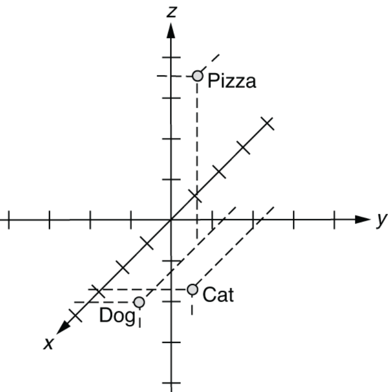
Figure 2.6 Word embeddings in a 3-D space

The x-axis (the first element) here represents some concept of “animal-ness” and the z-axis (the third dimension) corresponds to “food-ness.” (I’m making these numbers up, but you get the point.) This is essentially what word embeddings are. You just embedded those words in a three-dimensional space. By using those vectors, you already “know” how the basic building blocks of the language work. For example, if you wanted to identify animal names, then you would just look at the first element of each word vector and see if the value is high enough. This is a great jump start compared to the raw word indices!

You may be wondering where those numbers come from in practice. These numbers are actually “learned” using some machine learning algorithms and a large text dataset. We’ll discuss this further in chapter 3.

By the way, we have a much simpler method to “embed” words into a multidimensional space. Think of a multidimensional space that has as many dimensions as there are words. Then, give to each word a vector that is filled with zeros but just one 1, as shown next:

• vec("cat") = [1, 0, 0]

• vec("dog") = [0, 1, 0]

• vec("pizza") = [0, 0, 1]

Notice that each vector has only one 1 at the position corresponding to the word’s index. These special vectors are called one-hot vectors. These vectors are not very useful themselves in representing semantic relationship between those words—the three words are all at the equal distance from each other—but they are still (a very dumb kind of) embeddings. They are often used as the input to a machine learning algorithm when embeddings are not available.

2.3.2 Using word embeddings for sentiment analysis

First, we create dataset loaders that take care of loading data and passing it to the training pipeline, as shown next (more discussion on this data later in this chapter):

sampler = BucketBatchSampler(batch_size=32, sorting_keys=["tokens"])
train_data_loader = MultiProcessDataLoader(reader, train_path,
                                           batch_sampler=sampler)
dev_data_loader = MultiProcessDataLoader(reader, dev_path,
                                           batch_sampler=sampler)

AllenNLP provides a useful Vocabulary class that manages mappings from some linguistic units (such as characters, words, and labels) to their IDs. You can tell the class to create a Vocabulary instance from a set of instances as follows:

vocab = Vocabulary.from_instances(chain(train_data_loader.iter_instances(),
                                        dev_data_loader.iter_instances()),
                                  min_count={'tokens': 3})

Then, you need to initialize an Embedding instance, which takes care of converting IDs to embeddings, as shown in the next code snippet. The size (dimension) of the embeddings is determined by EMBEDDING_DIM:

token_embedding = Embedding(num_embeddings=vocab.get_vocab_size('tokens'),
                            embedding_dim=EMBEDDING_DIM)

Finally, you need to specify which index names correspond to which embeddings and pass it to BasicTextFieldEmbedder as follows:

word_embeddings = BasicTextFieldEmbedder({"tokens": token_embedding})

Now you can use word_embeddings to convert words (or more precisely, tokens, which I’ll talk more about in chapter 3) to their embeddings.

2.4 Neural networks

An increasingly large number of modern NLP applications are built using neural networks. You may have seen many amazing things that modern neural network models can achieve in the domain of computer vision and game playing (such as self-driving cars and Go-playing algorithms defeating human champions), and NLP is no exception. We are going to use neural networks for most of the NLP examples and applications we are going to build in this book. In this section, we discuss what neural networks are and why they are powerful.

2.4.1 What are neural networks?

Neural networks are at the core of modern NLP (and many other related AI fields, such as computer vision). It is such an important, vast research topic that it’d take a book (or maybe several books) to fully explain what it is and all the related models, algorithms, and so on. In this section, I’ll briefly explain the gist of it and will go into more details in later chapters as needed.

In short, a neural network (also called an artificial neural network) is a generic mathematical model that transforms a vector to another vector. That’s it. Contrary to what you may have read and heard in popular media, its essence is simple. If you are familiar with programming terms, think of it as a function that takes a vector, does some computation inside, and produces another vector as the return value. Then why is it such as big deal? How is it different from normal functions in programming?

The first difference is that neural networks are trainable. Think of it not just as a fixed function but more as a “template” for a set of related functions. If you use a programming language and write a function that includes several mathematical equations with some constants, you always get the same result if you feed the same input. On the contrary, neural networks can receive “feedback” (how close the output is to your desired output) and adjust their internal constants. Those “magic” constants are called weights or, more generally, parameters. Next time you run it, you expect that its answer is closer to what you want.

The second difference is its mathematical power. It’d be overly complicated if you were to use your favorite programming language and write a function that does, for example, sentiment analysis, if at all possible. (Remember the poor software engineer from chapter 1?) In theory, given enough model power and training data, neural networks are known to be able to approximate any continuous functions. This means that, whatever your problem is, neural networks can solve it if there’s a relationship between the input and the output and if you provide the model with enough computational power and training data.

Neural networks achieve this by learning functions that are not linear. What does it mean for a function to be linear? A linear function is a function where, if you change the input by x, the output will always change by c * x, where c is a constant number. For example, 2.0 * x is linear, because the return value always increases by 2.0 if you change x by 1.0. If you plot this on a graph, the relationship between the input and the output forms a straight line, which is why it’s called linear. On the other hand, 2.0 * x * x is not linear, because how much the return value changes depends not only on how much you change x but also on the value of x.

What this means is that a linear function cannot capture a more complex relationship between the input and the output and between the input variables. On the contrary, natural phenomena such as language are highly nonlinear. If you change the input by x (e.g., a word in a sentence), how much the output changes depends not only on how much x is changed but also on many other factors such as the value of x itself (e.g., what word you changed x to) and what other variables (e.g., the context of x) are. Neural networks, which are nonlinear mathematic models, have the potential to capture such complex interactions.

2.4.2 Recurrent neural networks (RNNs) and linear layers

Two special types of neural network components are important for sentiment analysis—recurrent neural networks (RNNs) and linear layers. I’ll explain them in detail in later chapters, but I’ll briefly describe what they are and their roles in sentiment analysis (or in general, sentence classification).

A recurrent neural network (RNN) is a neural network with loops, as shown in figure 2.7. It has an internal structure that is applied to the input again and again. Using the programming analogy, it’s like writing a function that contains for word in sentence: that loops over each word in the input sentence. It can either output the interim values of the internal variables of the loop, or the final values of the variables after the loop is finished, or both. If you just take the final values, you can use an RNN as a function that transforms a sentence to a vector with a fixed length. In many NLP tasks, you can use an RNN to transform a sentence to an embedding of the sentence. Remember word embeddings? They were fixed-length representation of words. Similarly, RNNs can produce fixed-length representation of sentences.

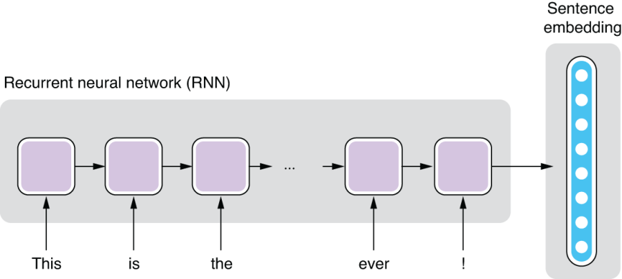
Figure 2.7 Recurrent neural network (RNN)

Another type of neural network component we’ll be using here is linear layers. A linear layer, also called a fully connected layer, transforms a vector to another vector in a linear fashion. As mentioned earlier, layer is just a fancier term for a substructure of neural networks, because you can stack them on top of each other to form a larger structure.

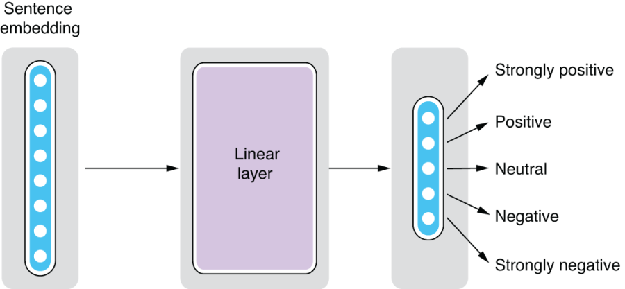
Remember, neural networks can learn nonlinear relationships between the input and the output. Why would we want something that is more constrained (linear) at all? Linear layers are used for compressing (or less often, expanding) vectors by reducing (or increasing) the dimensionality. For example, assume you receive a 64-dimensional vector (an array of 64 float numbers) from an RNN as a sentence embedding, but all you care about is a smaller number of values that are essential for your prediction. In sentiment analysis, you may care about only five values that correspond to five different sentiment labels, namely, strongly positive, positive, neutral, negative, and strongly negative. But you have no idea how to extract those five values from the embedded 64 values. This is exactly where a linear layer comes in handy—you can add a layer that transforms a 64-dimensional vector to a 5-dimensional one, and the neural networks figure out how to do that well, as shown in figure 2.8.

Figure 2.8 Linear layer

2.4.3 Architecture for sentiment analysis

Now you are ready to put the components together to build the neural network for the sentiment analyzer. First, you need to create the RNN as follows:

encoder = PytorchSeq2VecWrapper(
    torch.nn.LSTM(EMBEDDING_DIM, HIDDEN_DIM, batch_first=True))

Don’t worry too much about PytorchSeq2VecWrapper and batch_first=True. Here, you are creating an RNN (or more specifically, one type of RNN called LSTM, which stands for long short-term memory). The size of the input vector is EMBEDDING_DIM, which we saw earlier, and that of the output vector is HIDDEN_DIM.

Next, you need to create a linear layer, as shown here:

self.linear = torch.nn.Linear(in_features=encoder.get_output_dim(),
                              out_features=vocab.get_vocab_size('labels'))

The size of the input vector is defined by in_features, whereas out_features is that of the output vector. Because we are transforming the sentence embedding to a vector whose elements correspond to five sentiment labels, we need to specify the size of the encoder output and obtain the total number of labels from vocab.

Finally, we can connect those components and build a model as shown in the following code.

Listing 2.1 Building a sentiment analyzer model

class LstmClassifier(Model):
    def __init__(self,
                 word_embeddings: TextFieldEmbedder,
                 encoder: Seq2VecEncoder,
                 vocab: Vocabulary,
                 positive_label: str = '4') -> None:
        super().__init__(vocab)
        self.word_embeddings = word_embeddings
 
        self.encoder = encoder
 
        self.linear = torch.nn.Linear(in_features=encoder.get_output_dim(),
                                      out_features=vocab.get_vocab_size('labels'))
 
        self.loss_function = torch.nn.CrossEntropyLoss()         ❶
 
    def forward(self,                                            ❷
                tokens: Dict[str, torch.Tensor],
                label: torch.Tensor = None) -> torch.Tensor:
        mask = get_text_field_mask(tokens)
 
        embeddings = self.word_embeddings(tokens)
        encoder_out = self.encoder(embeddings, mask)
        logits = self.linear(encoder_out)
 
        output = {"logits": logits}
        if label is not None:
            self.accuracy(logits, label)
            self.f1_measure(logits, label)
            output["loss"] = self.loss_function(logits, label)   ❸
 
        return output

❶ Defines the loss function (cross entropy)

❷ The forward() function is where most of the computation happens in a model.

❸ Computes the loss and assigns it to the “loss” key of the returned dict

I want you to focus on the forward() function which is the most important function that every neural network model has. Its role is to take the input, pass it through subcomponents of the neural network, and produce the output. Although the function has some unfamiliar logics that we haven’t covered yet (such as mask and loss), what’s important here is the fact that you can chain the subcomponents of the model (word embeddings, RNN, and the linear layer) as if they were functions that transform the input (tokens), and you get something called logits at the end of the pipeline. Logit is a term in statistics that has a specific meaning, but here, you can think of it as something like a score for a class. The higher the score is for a specific label, the more confident that the label is the correct one.

2.5 Loss functions and optimization

Neural networks are trained using supervised learning. As mentioned earlier, supervised learning is a type of machine learning that learns a function that maps inputs to outputs based on a large amount of labeled data. So far, I covered only about how neural networks take an input and produce an output. How can we make it so that neural networks produce the output that we actually want?

Neural networks are not just like regular functions that you usually write in programming languages. They are trainable, meaning that they can receive some feedback and change their internal parameters so that they can produce more accurate outputs, even for the same inputs next time around. Notice there are two parts to this—receiving feedback and adjusting parameters, which are done through loss functions and optimization, respectively, which I’ll explain next.

A loss function is a function that measures how far an output of a machine learning model is from a desired one. The difference between an actual output and a desired one is called the loss. Loss is also called cost in some contexts. Either way, the bigger the loss, the worse it is, and you want it as close to zero as possible. Take sentiment analysis, for example. If the model thinks a sentence is 100% negative, but the training data says it’s strongly positive, the loss will be big. On the other hand, if the model thinks a sentence is maybe 80% negative and the training label is indeed negative, the loss will be small. It will be zero if both match exactly.

PyTorch provides a wide range of functions to compute losses. What we need here is called cross-entropy loss, which is often used for classification problems, as shown here:

self.loss_function = torch.nn.CrossEntropyLoss()

It can be used later by passing a prediction and labels from the training set as follows:

output["loss"] = self.loss_function(logits, label)

Then, this is where the magic happens. Neural networks, thanks to their mathematical properties, know how to change their internal parameters to make the loss smaller. Upon receiving some large loss, the neural network goes, “Oops, sorry, that was my mistake, but I’ll do better next round!” and changes its parameters. Remember I talked about a function that you write in a programming language that has some magic constants in it? Neural networks act like that function but know exactly how to change the magic constants to reduce the loss. They do this for each and every instance in the training data, so that they can produce more correct answers for as many instances as possible. Of course, they can’t reach the perfect answer after adjusting the parameters only once. It requires multiple passes, called epochs, over the training data. Figure 2.9 shows the overall training procedure for neural networks.

Figure 2.9 Overall training procedure for neural networks

The process where a neural network computes an output from an input using the current set of parameters is called the forward pass. This is why the main function in listing 2.1 is called forward(). The way the loss is fed back to the neural network is called backpropagation. An algorithm called stochastic gradient descent (SGD) is often used to minimize the loss. The process where the loss is minimized is called optimization, and the algorithm (such as SGD) used to achieve this is called the optimizer. You can initialize an optimizer using PyTorch as follows:

optimizer = optim.Adam(model.parameters())

Here, we are using one type of optimizer called Adam. There are many types of optimizers proposed in the neural network community, but the consensus is that there is no single optimization algorithm that works well for any problem, and you should be ready to experiment with multiple ones for your own problem.

OK, that was a lot of technical terms. You don’t need to know the details of those algorithms for now, but it’d be helpful if you learn just the terms and what they roughly mean. If you write the entire training process in Python pseudocode, it will appear as shown in listing 2.2. Note that there are two nested loops, one over epochs and another over instances.

Listing 2.2 Pseudocode for the neural network training loop

MAX_EPOCHS = 100
model = Model()
 
for epoch in range(MAX_EPOCHS):
    for instance, label in train_set:
        prediction = model.forward(instance)
        loss = loss_function(prediction, label)
        new_model = optimizer(model, loss)
        model = new_model

2.6 Training your own classifier

In this section, we are going to train our own classifier using AllenNLP’s training framework. I’ll also touch upon the concept of batching, an important practical concept that is used in training neural network models.

2.6.1 Batching

So far, I have left out one piece of detail—batching. We assumed that an optimization step happens for each and every instance, as you saw in the earlier pseudocode. In practice, however, we usually group a number of instances together and feed them to a neural network, updating model parameters per each group, not per each instance. We call this group of instances a batch.

Batching is a good idea for a couple of reasons. The first is stability. Any data is inherently noisy. Your dataset may contain sampling and labeling errors. If you update your model parameters for every instance, and if some instances contain errors, the update is influenced too much by the noise. But if you group instances into batches and compute the loss for the entire batch, not for individual instances, you can “average out” small errors and the feedback to your model stabilizes.

The second reason is speed. Training neural networks involves a huge number of arithmetic operations such as matrix additions and multiplications, and it is often done on GPUs (graphics processing units). Because GPUs are designed so that they can process a huge number of arithmetic operations in parallel, it is often efficient if you pass a large amount of data and process it at once instead of passing instances one by one. Think of a GPU as a factory overseas that manufactures products based on your specifications. Because factories are often optimized for manufacturing a small variety of products at a large quantity, and there is overhead in communicating and shipping products, it is more efficient if you make a small number of orders for manufacturing a large quantity of products instead of making a large number of orders for manufacturing a small quantity of products, even if you want the same quantity of products in total in either way.

It is easy to group instances into batches using AllenNLP. The framework uses PyTorch’s DataLoader abstraction, which takes care of receiving instances and returning batches. We’ll use a BucketBatchSampler that groups instances into buckets of similar lengths, as shown in the next code snippet. I’ll discuss why it’s important in later chapters:

sampler = BucketBatchSampler(batch_size=32, sorting_keys=["tokens"])
train_data_loader = MultiProcessDataLoader(reader, train_path, batch_sampler=sampler)
dev_data_loader = MultiProcessDataLoader(reader, dev_path, batch_sampler=sampler)

The parameter batch_size specifies the size of the batch (the number of instances in a batch). There is often a “sweet spot” in adjusting this parameter. It should be large enough to have any effect of the batching I mentioned earlier, but also small enough so that batches fit in the GPU memory, because factories have the maximum capacity of products they can manufacture at once.

2.6.2 Putting everything together

Now you are ready to train your sentiment analyzer. We assume that you already defined and initialized your model as follows:

model = LstmClassifier(word_embeddings, encoder, vocab)

See the full code listing (http://www.realworldnlpbook.com/ch2.html#sst-nb) for what the model looks like and how to use it.

AllenNLP provides the Trainer class, which acts as a framework for putting all the components together and managing the training pipeline, as shown here:

trainer = GradientDescentTrainer(
    model=model,
    optimizer=optimizer,
    data_loader=train_data_loader,
    validation_data_loader=dev_data_loader,
    patience=10,
    num_epochs=20,
    cuda_device=-1)
 
trainer.train()

You provide the model, optimizer, iterator, train set, dev set, and the number of epochs you want to the trainer and invoke the train method. The last parameter, cuda_device, tells the trainer which device (CPU or GPU) to use to use for training. Here, we are explicitly using the CPU. This will run the neural network training loop described in listing 2.2 and display the progress, including the evaluation metrics.

2.7 Evaluating your classifier

When training an NLP/ML model, you should always monitor how the loss changes over time. If the training is working as expected, you should see the loss decrease over time. It doesn’t always decrease each epoch, but it should decrease as a general trend, because this is exactly what you told the optimizer to do. If it’s increasing or showing weird values (such as NaN), it’s usually a sign that your model is too limiting or there’s a bug in your code.

In addition to the loss, it is important to monitor other evaluation metrics you care about in your task. Loss is a purely mathematical concept that measures the closeness between your model and the answer, but smaller losses do not always guarantee better performance in the NLP task.

You can use a number of evaluation metrics, depending on the nature of your NLP task, but some that you need to know no matter what task you are working on include accuracy, precision, recall, and F-measure. Roughly speaking, these metrics measure how precisely your model’s predictions match the expected answers defined by the dataset. For now, it suffices to know that they are used to measure how good your classifier is (more details coming in chapter 4).

To monitor and report evaluation metrics during training using AllenNLP, you need to implement the get_metrics() method in your model class, which returns a dict from metric names to their values, as shown next.

Listing 2.3 Defining evaluation metrics

   def get_metrics(self, reset: bool = False) -> Dict[str, float]:
        return {'accuracy': self.accuracy.get_metric(reset),
                **self.f1_measure.get_metric(reset)}

self.accuracy and self.f1_measure are defined in __init__() as follows:

    self.accuracy = CategoricalAccuracy()
    self.f1_measure = F1Measure(positive_index)

When you run trainer.train() with the metrics defined, you’ll see progress bars like these after every epoch:

accuracy: 0.7268, precision: 0.8206, recall: 0.8703, f1: 0.8448, batch_loss: 0.7609, loss: 0.7194 ||: 100%|##########| 267/267 [00:13<00:00, 19.28it/s]
accuracy: 0.3460, precision: 0.3476, recall: 0.3939, f1: 0.3693, batch_loss: 1.5834, loss: 1.9942 ||: 100%|##########| 35/35 [00:00<00:00, 119.53it/s]

You can see that the training framework reports these metrics both for the train and the validation sets. This is useful not only for evaluating your model but also for monitoring the progress of the training. If you see any unusual values, such as extremely low or high numbers, you’ll know that something is wrong, even before the training completes.

You may have noticed a large gap between the train and the validation metrics. Specifically, the metrics for the train set are a lot higher than those for the validation set. This is a common symptom of overfitting, which I mentioned earlier, where a model fits to a train set so well that it loses generalizability outside of it. This is why it’s important to monitor the metrics using a validation set as well, because you won’t know if it’s just doing well or overfitting only by looking at the training set metrics!

2.8 Deploying your application

The final step in making your own NLP application is deploying it. Training your model is only half the story. You need to set it up so that it can make predictions for new instances it has never seen. Making sure the model is serving predictions is critical in real-world NLP applications, and a lot of development efforts may go into this stage. In this section, I’m going to show what it’s like to deploy the model we just trained using AllenNLP. This topic is discussed in more detail in chapter 11.

2.8.1 Making predictions

To make predictions for new instances your model has never seen (called test instances), you need to pass them through the same neural network pipeline as you did for training. It has to be exactly the same—otherwise, you’ll risk skewing the result. This is called training-serving skew, which I’ll explain in chapter 11.

AllenNLP provides a convenient abstraction called predictors, whose job it is to receive an input in its raw form (e.g., raw string), pass it through the preprocessing and neural network pipeline, and give back the result. I wrote a specific predictor for SST called SentenceClassifierPredictor (http://realworldnlpbook.com/ch2 .html#predictor), which you can call as follows:

predictor = SentenceClassifierPredictor(model, dataset_reader=reader)
logits = predictor.predict('This is the best movie ever!')['logits']

Note that the predictor returns the raw output from the model, which is logits in this case. Remember, logits are some sort of scores corresponding to target labels, so if you want the predicted label itself, you need to convert it to the label. You don’t need to understand all the details for now, but this can be done by first taking the argmax of the logits, which returns the index of the logit with the maximum value, and then by looking up the label by the ID, as follows:

label_id = np.argmax(logits)
print(model.vocab.get_token_from_index(label_id, 'labels'))

If this prints out a “4,” congratulations! Label “4” corresponds to “very positive,” so your sentiment analyzer just predicted that the sentence “This is the best movie ever!” is very positive, which is indeed correct.

2.8.2 Serving predictions

Finally, you can easily deploy the trained model using AllenNLP. If you use a JSON configuration file (which I’ll explain in chapter 4), you can save your trained model onto disk and then quickly fire up a web-based interface where you can make requests to your model. To do this, you need to install allennlp-server, a plugin for AllenNLP that provides a web interface for prediction, as follows:

git clone https:/./github.com/allenai/allennlp-server
pip install —editable allennlp-server

Assuming your model is saved under examples/sentiment/model, you can run a Python-based web application using the following AllenNLP command:

$ allennlp serve  
    --archive-path examples/sentiment/model/model.tar.gz 
    --include-package examples.sentiment.sst_classifier 
    --predictor sentence_classifier_predictor 
    --field-name sentence

If you open http:/./localhost:8000/ using your browser, you’ll see the interface shown in figure 2.10.

Figure 2.10 Running the sentiment analyzer on a web browser

Try typing some sentences in the sentence text box, and click Predict. You should see the logits values on the right side of the screen. They are just a raw array of logits and hard to read, but you can see that the fourth value (which corresponds to the label “very positive”) is the largest and the model is working as expected.

You can also directly make POST requests to the backend from the command line as follows:

curl -d '{"sentence": "This is the best movie ever!"}'
    -H "Content-Type: application/json" 
    -X POST http:/./localhost:8000/predict

This should return the same JSON as you saw above:

{"logits":[-0.2549717128276825,-0.35388273000717163,
-0.0826418399810791,0.7183976173400879,0.23161858320236206]}

OK, that’s it for now. We covered a lot in this chapter, but don’t worry—I just wanted to show you that it is easy to build an NLP application that actually works. You may have found some books or online tutorials about neural networks and deep learning intimidating, or you may have even given up on learning before creating anything that works. Notice that I didn’t even mention any concepts such as neurons, activations, gradient, and partial derivatives, which other learning materials teach at the very beginning. These concepts are indeed important and helpful to know, but thanks to powerful frameworks such as AllenNLP, you are also able to build practical NLP applications without fully understanding their details. In later chapters, I’ll go into more details and discuss these concepts as needed.

Summary

• Sentiment analysis is a text analytic technique to automatically identify subjective information within text, such as its polarity (positive or negative).

• Train, dev, and test sets are used to train, choose, and evaluate machine learning models.

• Word embeddings represent the meaning of words using vectors of real numbers.

• Recurrent neural networks (RNNs) and linear layers are used to convert a vector to another vector of different size.

• Neural networks are trained using an optimizer so that the loss (discrepancy between the actual and the desired output) is minimized.

• It is important to monitor the metrics for the train and the dev sets during training to avoid overfitting.