
8 Attention and Transformer
- Using attention to produce summaries of the input and improve the quality of Seq2Seq models
- Replacing RNN-style loops with self-attention, a mechanism for the input to summarize itself
- Improving machine translation systems with the Transformer model
- Building a high-quality spell-checker using the Transformer model and publicly available datasets
Our focus so far in this book has been recurrent neural networks (RNNs), which are a powerful model that can be applied to various NLP tasks such as sentiment analysis, named entity recognition, and machine translation. In this chapter, we will introduce an even more powerful model—the Transformer1—a new type of encoder-decoder neural network architecture based on the concept of self-attention. It is without a doubt the most important NLP model since it appeared in 2017. Not only is it a powerful model itself (for machine translation and various Seq2Seq tasks, for example), but it is also used as the underlying architecture that powers numerous modern NLP pretrained models, including GPT-2 (section 8.4.3) and BERT (section 9.2). The developments in modern NLP since 2017 can be best summarized as “the era of the Transformer.”
In this chapter, we start with attention, a mechanism that made a breakthrough in machine translation, then move on to introducing self-attention, the concept that forms the foundation of the Transformer model. We will build two NLP applications—a Spanish-to-English machine translator and a high-quality spell-checker—and learn how to apply the Transformer model to your everyday applications. As we’ll see later, the Transformer models can improve the quality of NLP systems over RNNs by a large margin and achieve almost human-level performance in some tasks, such as translation and generation.
8.1 What is attention?
In chapter 6, we covered Seq2Seq models—NLP models that transform one sequence to another using an encoder and a decoder. Seq2Seq is a versatile and powerful paradigm with many applications, although the “vanilla” Seq2Seq models are not without limitation. In this section, we discuss the Seq2Seq models’ bottleneck and motivate the use of an attention mechanism.
8.1.1 Limitation of vanilla Seq2Seq models
Let’s remind ourselves how Seq2Seq models work. Seq2Seq models consist of an encoder and a decoder. The decoder takes a sequence of tokens in the source language and runs it through an RNN, which produces a fixed-length vector at the end. This fixed-length vector is a representation of the input sentence. The decoder, which is another RNN, takes this vector and produces a sequence in the target language, token by token. Figure 8.1 illustrates how Spanish sentences are translated into English with a vanilla Seq2Seq model.
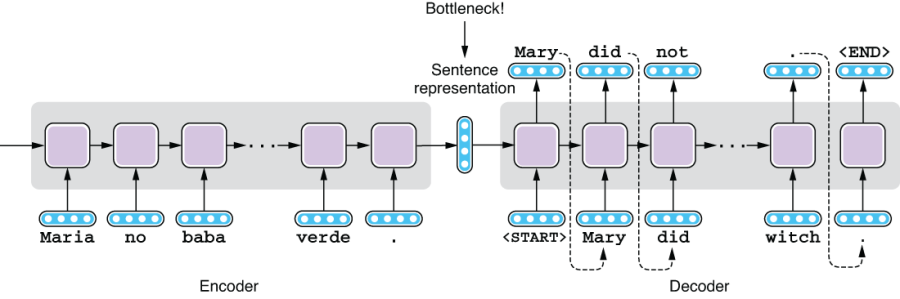
Figure 8.1 A bottleneck in a vanilla Seq2Seq model
This Seq2Seq architecture is quite simple and powerful, but it is known that its vanilla version (shown in figure 8.1) does not translate sentences as well as other traditional machine translation algorithms (such as phrase-based statistical machine translation models). You may be able to guess why this is the case if you look at its structure carefully—its encoder is trying to “compress” all the information in the source sentence into the sentence representation, which is a vector of some fixed length (e.g., 256 floating-point numbers), and the decoder is trying to restore the entire target sentence just from that vector. The size of the vector is fixed no matter how long (or how short) the source sentence is. The intermediate vector is a huge bottleneck. If you think of how humans actually translate between languages, this sounds quite difficult and somewhat unusual. Professional translators do not just read the source sentence and write down its translation in one breath. They refer to the source sentences as many times as necessary to translate the relevant parts in the target sentence.
Compressing all the information into one vector may (and does) work for short sentences, as we’ll see later in section 8.2.2, but it becomes increasingly difficult as the sentences get longer and longer. Studies have shown that the translation quality of a vanilla Seq2Seq model gets worse as the sentence gets longer.2
8.1.2 Attention mechanism
Instead of relying on a single, fixed-length vector to represent all the information in a sentence, the decoder would have a much easier time if there was a mechanism where it can refer to some specific part of the encoder as it generates the target tokens. This is similar to how human translators (the decoder) reference the source sentence (the encoder) as needed.
This can be achieved by using attention, which is a mechanism in neural networks that focuses on a specific part of the input and computes its context-dependent summary. It is like having some sort of key-value store that contains all of the input’s information and then looking it up with a query (the current context). The stored values are not just a single vector but usually a list of vectors, one for each token, associated with corresponding keys. This effectively increases the size of the “memory” the decoder can refer to when it’s making a prediction.
Before we discuss how the attention mechanism works for Seq2Seq models, let’s see it in action in a general form. Figure 8.2 illustrates a generic attention mechanism with the following features:
-
The inputs to an attention mechanism are the values and their associated keys. The input values can take many different forms, but in NLP, they are almost always lists of vectors. For Seq2Seq models, the keys and values here are the hidden states of the encoder, which represent token-by-token encoding of the input sentence.
-
Each key associated with a value is compared against the query using an attention function f. By applying f to the query and each one of the keys, you get a set of scores, one per key-value pair, which are then normalized to obtain a set of attention weights. The specific function f depends on the architecture (more on this later). For Seq2Seq models, this gives you a distribution over the input tokens. The more relevant an input token is, the larger the weight it gets.
-
The input values are weighted by their corresponding weights obtained in step 2 and summed up to compute the final summary vector. For Seq2Seq models, this summary vector is appended to the decoder hidden states to aid the translation process.

Figure 8.2 Using an attention mechanism to summarize the input
Because of step 3, the output of an attention mechanism is always a weighted sum of the input vectors, but how they are weighted is determined by the attention weights, which are in turn are calculated from the keys and the query. In other words, what an attention mechanism computes is a context (query)-dependent summary of the input. Downstream components of a neural network (e.g., the decoder of an RNN-based Seq2Seq model, or the upper layers of a Transformer model) use this summary to further process the input.
In the following sections, we will learn the two most commonly used types of attention mechanisms in NLP—encoder-decoder attention (also called cross-attention; used in both RNN-based Seq2Seq models and the Transformer) and self-attention (used in the Transformer).
8.2 Sequence-to-sequence with attention
In this section, we’ll learn how the attention mechanism is applied to an RNN-based Seq2Seq model for which the attention mechanism was first invented. We’ll study how it works with specific examples, and then we’ll experiment with Seq2Seq models with and without the attention mechanism using fairseq to observe how it affects the translation quality.
8.2.1 Encoder-decoder attention
As we saw earlier, attention is a mechanism for creating a summary of the input under a specific context. We used a key-value store and a query as an analogy for how it works. Let’s see how an attention mechanism is used with RNN-based Seq2Seq models using the concrete examples that follow.

Figure 8.3 Adding an attention mechanism to an RNN-based Seq2Seq model (the lightly shaded box)
Figure 8.3 illustrates a Seq2Seq model with attention. It looks complex at first, but it is just an RNN-based Seq2Seq model with some extra “things” added on top of the encoder (the lightly shaded box in top left corner of the figure). If you ignore what’s inside and see it as a black box, all it does is simply take a query and return some sort of summary created from the input. The way it computes this summary is just a variant of the generic form of attention we covered in section 8.1.2. It proceeds as follows:
-
The input to the attention mechanism is the list of hidden states computed by the encoder. These hidden states are used as both keys and values (i.e., the keys and the values are identical). The encoder hidden state at a certain token (e.g., at token “no”) reflects the information about that token and all the tokens leading up to it (if the RNN is unidirectional) or the entire sentence (if the RNN is bidirectional).
-
Let’s say you finished decoding up to “Mary did.” The hidden states of the decoder at that point are used as the query, which is compared against every key using function f. This produces a list of attention scores, one per each key-value pair. These scores determine which part of the input the decoder should attend to when it’s trying to generate a word that follows “Mary did.”
- These scores are converted to a probability distribution (a set of positive values that sum to one), which is used to determine which vectors should get the most attention. The return value from this attention mechanism is the sum of all values, weighted by the attention scores after normalizing with softmax.
You may be wondering what the attention function f looks like. A couple of variants of f are possible, depending on how it computes the attention scores between the key and the query, but these details do not matter much here. One thing to note is that in the original paper proposing the attention mechanism,3 the authors used a “mini” neural network to calculate attention scores from the key and the query.
This “mini” network-based attention function is not something you just plug in to an RNN model post hoc and expect it to work. It is optimized as part of the entire network—that is, as the entire network gets optimized by minimizing the loss function, the attention mechanism also gets better at generating summaries because doing so well also helps the decoder generate better translation and lower the loss function. In other words, the entire network, including the attention mechanism, is trained end to end. This usually means that, as the network is optimized, the attention mechanism starts to learn to focus only on the relevant part of the input, which is usually where the target tokens are aligned with the source tokens. In other words, attention is calculating some sort of “soft” word alignment between the source and the target tokens.
8.2.2 Building a Seq2Seq machine translation with attention
In section 6.3, we built our first machine translation (MT) system using fairseq, an NMT toolkit developed by Facebook. Using the parallel dataset from Tatoeba, we built an LSTM-based Seq2Seq model to translate Spanish sentences into English.
In this section, we are going to experiment with a Seq2Seq machine translation system and see how attention affects the translation quality. We assume that you’ve already gone through the steps we took when we built the MT system by downloading the dataset and running the fairseq-preprocess and fairseq-train commands (section 6.3). After that, you ran the fairseq-interactive command to interactively translate Spanish sentences into English. You might have noticed that the translation you get from this MT system that took you just 30 minutes to build was actually decent. In fact, the model architecture we used (—arch lstm) has an attention mechanism built in by default. Notice when you ran the following fairseq-train command
fairseq-train
    data/mt-bin
    --arch lstm
    --share-decoder-input-output-embed
    --optimizer adam
    --lr 1.0e-3
    --max-tokens 4096
    --save-dir data/mt-ckpt
you should have seen the dump of what your model looks like in your terminal as follows:
...
LSTMModel(
  (encoder): LSTMEncoder(
    (embed_tokens): Embedding(16832, 512, padding_idx=1)
    (lstm): LSTM(512, 512)
  )
  (decoder): LSTMDecoder(
    (embed_tokens): Embedding(11416, 512, padding_idx=1)
    (layers): ModuleList(
      (0): LSTMCell(1024, 512)
    )
    (attention): AttentionLayer(
      (input_proj): Linear(in_features=512, out_features=512, bias=False)
      (output_proj): Linear(in_features=1024, out_features=512, bias=False)
    )
  )
)
...
This tells you that your model has an encoder and a decoder, but the decoder also has a component called attention (which is of type AttentionLayer), shown in bold in the code snippet. This is exactly the “mini-network” that we covered in section 8.2.1.
Now let’s train the same model, but without attention. You can add —decoder-attention 0 to fairseq-train to disable the attention mechanism, while keeping everything else the same, as shown here:
$ fairseq-train
      data/mt-bin
      --arch lstm
      --decoder-attention 0
      --share-decoder-input-output-embed
      --optimizer adam
      --lr 1.0e-3
      --max-tokens 4096
      --save-dir data/mt-ckpt-no-attn
When you run this, you’ll see a similar dump, shown next, that shows the architecture of the model but without attention:
LSTMModel(
  (encoder): LSTMEncoder(
    (embed_tokens): Embedding(16832, 512, padding_idx=1)
    (lstm): LSTM(512, 512)
  )
  (decoder): LSTMDecoder(
    (embed_tokens): Embedding(11416, 512, padding_idx=1)
    (layers): ModuleList(
      (0): LSTMCell(1024, 512)
    )
  )
)
As we saw in section 6.3.2, the training process alternates between training and validation. In the training phase, the parameters of the neural network are optimized by the optimizer. In the validation phase, these parameters are fixed, and the model is run on a held-out portion of the dataset called the validation set. In addition to making sure the training loss decreases, you should be looking at the validation loss during training, because it better represents how well the model generalizes outside the training data.
During this experiment, you should observe that the lowest validation loss achieved by the attention model is around 1.727, whereas that for the attention-less model is around 2.243. Lower loss values mean the model is fitting the dataset better, so this indicates the attention is helping improve the translation. Let’s see if this is actually the case. As we’ve done in section 6.3.2, you can generate translations interactively by running the following fairseq-interactive command:
$ fairseq-interactive
    data/mt-bin
    --path data/mt-ckpt/checkpoint_best.pt
    --beam 5
    --source-lang es
    --target-lang en
In table 8.1, we compare the translations generated by the model with and without attention. The translations you get from the attention-based model are the same as the ones we saw in section 6.3.3. Notice that the translations you get from the attention-less model are a lot worse than those from the attention model. If you look at the translations for “¿Hay habitaciones libres?” and “Maria no daba una bofetada a la bruja verde,” you see unfamiliar tokens “<unk>” (for “unknown”) in them. What’s happening here?
Table 8.1 Translation generated by the model with and without attention
These are special tokens that are assigned to out-of-vocabulary (OOV) words. We touched upon OOV words in section 3.6.1 (when we introduced the concept of subwords used for FastText). Most NLP applications operate within a fixed vocabulary, and whenever they encounter or try to produce words that are outside that predefined set, the words are replaced with a special token, <unk>. This is akin to a special value (such as None in Python) returned when a method doesn’t know what to do with the input. Because these sentences contain certain words (I suspect they are “libres” and “bofetada”), the Seq2Seq model without attention, whose memory is limited, didn’t know what to do with them and simply fell back on a safest thing to do, which is to produce a generic, catch-all symbol, <unk>. On the other hand, you can see that attention prevents the system from producing these symbols and helps improve the overall quality of the produced translations.
8.3 Transformer and self-attention
In this section, we are going to learn how the Transformer model works and, specifically, how it generates high-quality translations by using a new mechanism called self-attention. Self-attention creates a summary of the entire input, but it does this for each token using the token as the context.
8.3.1 Self-attention
As we’ve seen before, attention is a mechanism that creates a context-dependent summary of the input. For RNN-based Seq2Seq models, the input is the encoder hidden states, whereas the context is the decoder hidden states. The core idea of the Transformer, self-attention, also creates a summary of the input, except for one key difference—the context in which the summary is created is also the input itself. See figure 8.4 for a simplified illustration of a self-attention mechanism.

Figure 8.4 Self-attention transforms the input into summaries.
Why is this a good thing? Why does it even work? As we discussed in chapter 4, RNNs can also create a summary of the input by looping over the input tokens while updating an internal variable (hidden states). This works—we previously saw that RNNs can generate good translations when combined with attention, but they have one critical issue: because RNNs process the input sequentially, it becomes progressively more difficult to deal with long-range dependencies between tokens as the sentence gets longer.
Let’s look at a concrete example. If the input sentence is “The Law will never be perfect, but its application should be just,” understanding what the pronoun “its” refers to (“The Law”) is important for understanding what the sentence means and for any subsequent tasks (such as translating the sentence accurately). However, if you use an RNN to encode this sentence, to learn this coreference relationship, the RNN needs to learn to remember the noun “The Law” in the hidden states first, then wait until the loop encounters the target pronoun (“its”) while learning to ignore everything unrelated in between. This sounds like a complicated trick for a neural network to learn.
But things shouldn’t be that complicated. Singular possessive pronouns like “its” usually refer to their nearest singular nouns that appear before them, regardless of the words in between, so simple rules like “replace it with the nearest noun that appeared before” will suffice. In other words, such “random access” is better suited in this situation than “sequential access” is. Self-attention is better at learning such long-range dependencies, as we’ll see later.
Let’s walk through how self-attention works with an example. Let’s assume we are translating Spanish into English and would like to encode the first few words, “Maria no daba,” in the input sentence. Let’s also focus on one specific token, “no,” and how its embeddings are computed from the entire input. The first step is to compare the target token against all tokens in the input. Self-attention does this by converting the target into a query by using projection WQ as well as converting all the tokens into keys using projection WK and computing attention weights using function f. The attention weights computed by f are normalized and converted to a probability distribution by the softmax function. Figure 8.5 illustrates these steps where attention weights are computed. As with the encoder-decoder attention mechanism we covered in section 8.2.1, these weights determine how to “mix” values we obtained from the input tokens. For words like “its,” we expect that the weight will be higher for related words such as “Law” in the example shown earlier.
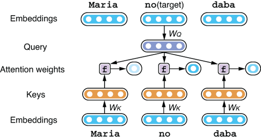
Figure 8.5 Computing attention weights from keys and queries
In the next step, the vector corresponding to each input token is converted to a value vector by projection WV. Each projected value is weighted by the corresponding attention weight and is summed up to produce a summary vector. See figure 8.6 for an illustration.

Figure 8.6 Calculating the sum of all values weighted by attention weights
This would be it if this were the “regular” encoder-decoder attention mechanism. You need only one summary vector per each token during decoding. However, one key difference between encoder-decoder attention and self-attention is the latter repeats this process for every single token in the input. As shown in figure 8.7, this produces a new set of embeddings for the input, one for each token.

Figure 8.7 Producing summaries for the entire input sequence (details are omitted)
Each summary produced by self-attention takes all the tokens in the input sequence into consideration, but with different weights. It is, therefore, straightforward for words like “its” to incorporate some information from related words, such as “The Law,” no matter how far apart these two words are. Using an analogy, self-attention produces summaries through random access over the input. This is in contrast to RNNs, which allow only sequential access over the input, and is one of the key reasons why the Transformer is such a powerful model for encoding and decoding natural language text.
We need to cover one final piece of detail to fully understand self-attention. As it is, the self-attention mechanism illustrated previously can use only one aspect of the input sequence to generate summaries. For example, if you want self-attention to learn which word each pronoun refers to, it can do that—but you may also want to “mix in” information from other words based on some other linguistic aspects. For example, you may want to refer to some other words that the pronoun modifies (“applications,” in this case). The solution is to have multiple sets of keys, values, and queries per token and compute multiple sets of attention weights to “mix” values that focus on different aspects of the input. The final embeddings are a combination of summaries generated this way. This mechanism is called multihead self-attention (figure 8.8).
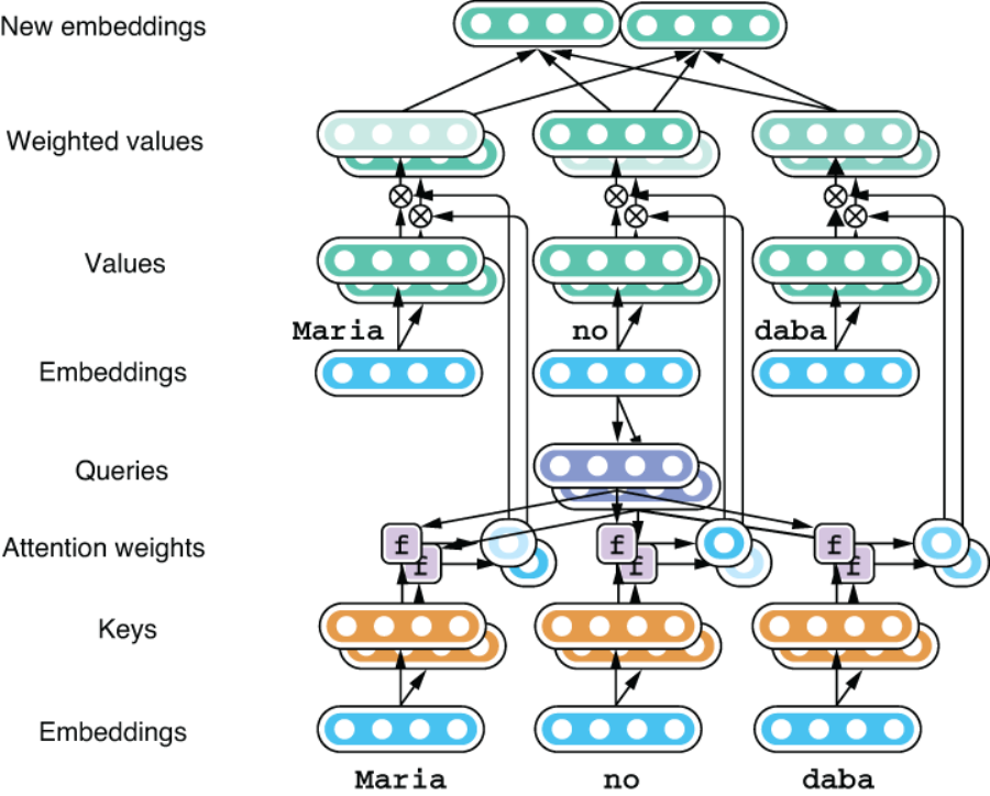
Figure 8.8 Multihead self-attention produces summaries with multiple keys, values, and queries.
You would need to learn some additional details if you were to fully understand how a Transformer layer works, but this section has covered the most important concepts. If you are interested in more details, check out The Illustrated Transformer (http://jalammar.github.io/illustrated-transformer/), a well-written guide for understanding the Transformer model with easy-to-understand illustrations. Also, if you are interested in implementing the Transformer model from scratch in Python, check out “The Annotated Transformer” (http://nlp.seas.harvard.edu/2018/04/03/attention.html).
8.3.2 Transformer
The Transformer model doesn’t just use a single step of self-attention to encode or decode natural language text. It applies self-attention repeatedly to the inputs to gradually transform them. As with multilayer RNNs, the Transformer also groups a series of transformation operations into a layer and applies it repeatedly. Figure 8.9 shows one layer of the Transformer encoder.
A lot is going on within each layer, and it’s not our goal to explain every bit of its detail—you need to understand only that the multihead self-attention is at its core, followed by transformation by a feed-forward neural network (“FF” in figure 8.9). Residual connections and normalization layers are introduced to make it easier to train the model, although the details of these operations are outside the scope of this book. The Transformer model applies this layer repeatedly to transform the input from something literal (raw word embeddings) to something more abstract (the “meaning” of the sentence). In the original Transformer paper, Vaswani et al. used six layers for machine translation, although it is not uncommon for larger models to use 10-20 layers these days.
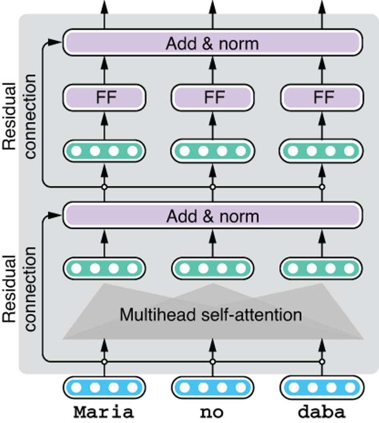
Figure 8.9 A Transformer encoder layer with self-attention and a feed-forward layer
At this point, you may have noticed that the self-attention operation is completely independent of positions. In other words, the embedded results of self-attention would be completely identical even if, for example, we flipped the word order between “Maria” and “daba,” because the operation looks only at the word itself and the aggregated embeddings from other words, regardless of where they are. This is obviously very limiting—what a natural language sentence means depends a lot on how its words are ordered. How does the Transformer encode word order, then?
The Transformer model solves this problem by generating some artificial embeddings that differ from position to position and adding them to word embeddings before they are fed to the layers. These embeddings, called positional encoding and shown in figure 8.10, are either generated by some mathematical function (such as sine curves) or learned during training per position. This way, the Transformer can distinguish between “Maria” at the first position and “Maria” at the third position, because they have different positional encoding.
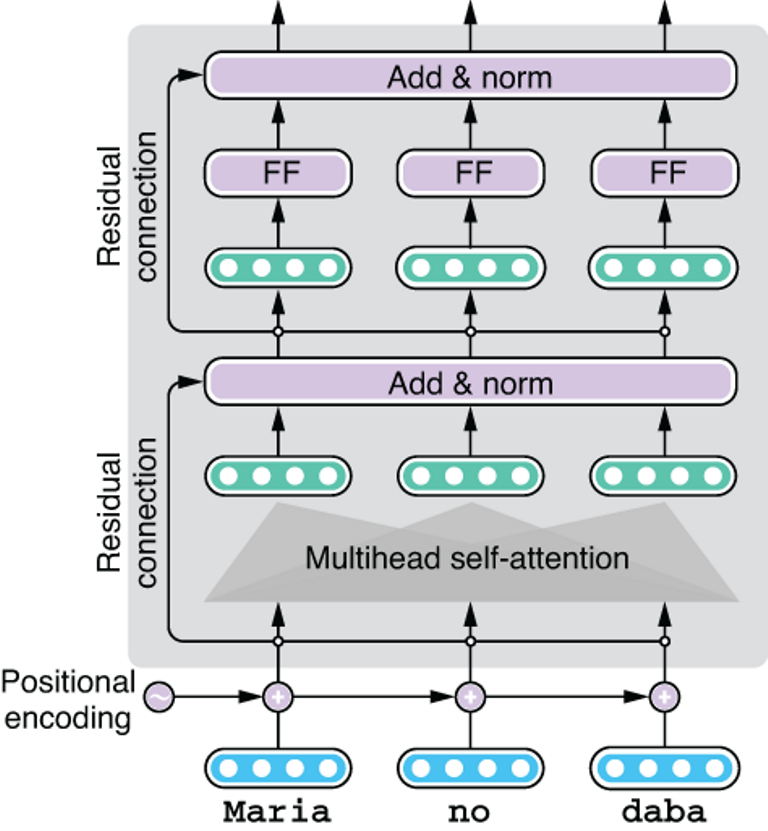
Figure 8.10 Adding positional encoding to the input to represent word order
Figure 8.11 shows the Transformer decoder. Although a lot is going on, make sure to notice two important things. First, you’ll notice one extra mechanism called cross-attention inserted between the self-attention and feed-forward networks. This cross-attention mechanism is similar to the encoder-decoder attention mechanism we covered in section 8.2. This works exactly the same as self-attention, except that the values for the attention come from the encoder, not the decoder, summarizing the information extracted from the encoder.

Figure 8.11 A Transformer decoder layer with self- and cross-attention
Finally, the Transformer model generates the target sentence in exactly the same way as RNN-based Seq2Seq models we’ve previously learned in section 6.4. The decoder is initialized by a special token <START> and produces a probability distribution over possible next tokens. From here, you can proceed by choosing the token with the maximum probability (greedy decoding, as shown in section 6.4.3) or keeping a few tokens with the highest probability while searching for the path that maximizes the total score (beam search, as shown in section 6.4.4). In fact, if you look at the Transformer decoder as a black box, the way it produces the target sequence is exactly the same as RNNs, and you can use the same set of decoding algorithms. In other words, the decoding algorithms covered in section 6.4 are generic ones that are agnostic of the underlying decoder architecture.
8.3.3 Experiments
Now that we know how the Transformer model works, let’s build a machine translation system with it. The good news is the sequence-to-sequence toolkit, Fairseq, already supports the Transformer-based models (along with other powerful models), which can be specified by the —arch transformer option when you train the model. Assuming that you have already preprocessed the dataset we used to build the Spanish-to-English machine translation, you need to tweak only the parameters you give to fairseq-train, as shown next:
fairseq-train
  data/mt-bin
  --arch transformer
  --share-decoder-input-output-embed
  --optimizer adam --adam-betas '(0.9, 0.98)' --clip-norm 0.0
  --lr 5e-4 --lr-scheduler inverse_sqrt --warmup-updates 4000
  --dropout 0.3 --weight-decay 0.0
  --criterion label_smoothed_cross_entropy --label-smoothing 0.1
  --max-tokens 4096
  --save-dir data/mt-ckpt-transformer
Note that this might not even run on your laptop. You really need GPUs to train the Transformer models. Also note that training can take hours even with GPUs. See section 11.5 for more information on using GPUs.
A number of cryptic parameters appear here, but you don’t need to worry about them. You can see the model structure when you run this command. The entire model dump is quite long, so we are omitting some intermediate layers in listing 8.1. If you look carefully, you’ll see that the structure of the layers corresponds to the figures we showed earlier.
Listing 8.1 Transformer model dump from Fairseq
TransformerModel(
  (encoder): TransformerEncoder(
    (embed_tokens): Embedding(16832, 512, padding_idx=1)
    (embed_positions): SinusoidalPositionalEmbedding()
    (layers): ModuleList(
      (0): TransformerEncoderLayer(
        (self_attn): MultiheadAttention(                                   ❶
          (out_proj): Linear(in_features=512, out_features=512, bias=True)
        )
        (self_attn_layer_norm): LayerNorm((512,), eps=1e-05, elementwise_
         affine=True)
        (fc1): Linear(in_features=512, out_features=2048, bias=True)       ❷
        (fc2): Linear(in_features=2048, out_features=512, bias=True)
        (final_layer_norm): LayerNorm((512,), eps=1e-05, elementwise_affine=True)
      )
      ...
      (5): TransformerEncoderLayer(
        (self_attn): MultiheadAttention(
          (out_proj): Linear(in_features=512, out_features=512, bias=True)
        )
        (self_attn_layer_norm): LayerNorm((512,), eps=1e-05, elementwise_affine=True)
        (fc1): Linear(in_features=512, out_features=2048, bias=True)
        (fc2): Linear(in_features=2048, out_features=512, bias=True)
        (final_layer_norm): LayerNorm((512,), eps=1e-05, elementwise_affine=True)
      )
    )
  )
  (decoder): TransformerDecoder(
    (embed_tokens): Embedding(11416, 512, padding_idx=1)
    (embed_positions): SinusoidalPositionalEmbedding()
    (layers): ModuleList(
      (0): TransformerDecoderLayer(
        (self_attn): MultiheadAttention(                                   ❸
          (out_proj): Linear(in_features=512, out_features=512, bias=True)
        )
        (self_attn_layer_norm): LayerNorm((512,), eps=1e-05, elementwise_affine=True)
        (encoder_attn): MultiheadAttention(                                ❹
          (out_proj): Linear(in_features=512, out_features=512, bias=True)
        )
        (encoder_attn_layer_norm): LayerNorm((512,), eps=1e-05, elementwise_
         affine=True)
        (fc1): Linear(in_features=512, out_features=2048, bias=True)       ❺
        (fc2): Linear(in_features=2048, out_features=512, bias=True)
        (final_layer_norm): LayerNorm((512,), eps=1e-05, elementwise_affine=True)
      )
      ...
      (5): TransformerDecoderLayer(
        (self_attn): MultiheadAttention(
          (out_proj): Linear(in_features=512, out_features=512, bias=True)
        )
        (self_attn_layer_norm): LayerNorm((512,), eps=1e-05, elementwise_affine=True)
        (encoder_attn): MultiheadAttention(
          (out_proj): Linear(in_features=512, out_features=512, bias=True)
        )
        (encoder_attn_layer_norm): LayerNorm((512,), eps=1e-05, elementwise_
         affine=True)
        (fc1): Linear(in_features=512, out_features=2048, bias=True)
        (fc2): Linear(in_features=2048, out_features=512, bias=True)
        (final_layer_norm): LayerNorm((512,), eps=1e-05, elementwise_affine=True)
      )
    )
  )
)
❶ Self-attention of the encoder
❷ Feed-forward network of the encoder
❸ Self-attention of the decoder
❹ Encoder-decoder of the decoder
❺ Feed-forward network of the decoder
When I ran this, the validation loss converges after around epoch 30, at which point you can stop the training. The result I got by translating the same set of Spanish sentences into English follows:
¡ Buenos días !
S-0     ¡ Buenos días !
H-0     -0.0753164291381836     Good morning !
P-0     -0.0532 -0.0063 -0.1782 -0.0635
¡ Hola !
S-1     ¡ Hola !
H-1     -0.17134985327720642    Hi !
P-1     -0.2101 -0.2405 -0.0635
¿ Dónde está el baño ?
S-2     ¿ Dónde está el baño ?
H-2     -0.2670585513114929     Where 's the toilet ?
P-2     -0.0163 -0.4116 -0.0853 -0.9763 -0.0530 -0.0598
¿ Hay habitaciones libres ?
S-3     ¿ Hay habitaciones libres ?
H-3     -0.26301929354667664    Are there any rooms available ?
P-3     -0.1617 -0.0503 -0.2078 -1.2516 -0.0567 -0.0532 -0.0598
¿ Acepta tarjeta de crédito ?
S-4     ¿ Acepta tarjeta de crédito ?
H-4     -0.06886537373065948    Do you accept credit card ?
P-4     -0.0140 -0.0560 -0.0107 -0.0224 -0.2592 -0.0606 -0.0594
La cuenta , por favor .
S-5     La cuenta , por favor .
H-5     -0.08584468066692352    The bill , please .
P-5     -0.2542 -0.0057 -0.1013 -0.0335 -0.0617 -0.0587
Maria no daba una bofetada a la bruja verde .
S-6     Maria no daba una bofetada a la bruja verde .
H-6     -0.3688890039920807     Mary didn 't slapped the green witch .
P-6     -0.2005 -0.5588 -0.0487 -2.0105 -0.2672 -0.0139 -0.0099 -0.1503 -0.0602
You can see most of these English translations here are almost perfect. It is quite surprising that the model translated the most difficult sentence (“Maria no daba . . .”) almost perfectly. This is probably enough to convince us that the Transformer is a powerful translation model. After its advent, this model became the de facto standard in research and commercial machine translation.
8.4 Transformer-based language models
In section 5.5, we introduced language models, which are statistical models that give a probability to a piece of text. By decomposing text into a sequence of tokens, language models can estimate how “probable” the given text is. In section 5.6, we demonstrated that by leveraging this property, language models can also be used to generate new texts out of thin air!
The Transformer is a powerful model that achieves impressive results in Seq2Seq tasks (such as machine translation), although its architecture can also be used for modeling and generating language. In this section, we learn how to use the Transformer for modeling language and generating realistic texts.
8.4.1 Transformer as a language model
In section 5.6, we built a language-generation model based on a character LSTM-RNN. To recap, given a prefix (a partial sentence generated so far), the model uses an LSTM-based RNN (a neural network with a loop) to produce a probability distribution over possible next tokens, as shown in figure 8.12.

Figure 8.12 Generating text using an RNN
We noted earlier that, by regarding the Transformer decoder as a black box, you can use the same set of decoding algorithms (greedy, beam search, and so on) as we introduced earlier for RNNs. This is also the case for language generation—by thinking of the neural network as a black box that produces some sort of score given a prefix, you can use the same logic to generate texts, no matter the underlying model. Figure 8.13 shows how an architecture similar to the Transformer can be used for language generation. Except for a few minor differences (such as lack of cross-attention), the structure is almost identical to the Transformer decoder.

Figure 8.13 Using the Transformer for language generation
The following snippet shows Python-like pseudocode for generating text with the Transformer model. Here, model() is the main function where the model computation happens—it takes the tokens, converts them to embeddings, adds positional encoding, and passes them through all the Transformer layers, returning the final hidden states back to the caller. The caller then passes them through a linear layer to convert them to logits, which in turn get converted to a probability distribution by softmax:
def generate():
    token = <START>
    tokens = [<START>]
    while token != <END>:
        hidden = model(tokens)
        probs = softmax(linear(hidden))
        token = sample(probs)
        tokens.append(token)
    return tokens
In fact, decoding for Seq2Seq models and language generation with language models are very similar tasks, where the output sequence is produced token by token, feeding itself back to the network, as shown in the previous code snippet. The only difference is that the former has some form of input (the source sentence) whereas the latter does not (the model feeds itself). These two tasks are also called unconditional and conditional generation, respectively. Figure 8.14 illustrates these three components (network, task, and decoding) and how they can be combined to solve a specific problem.
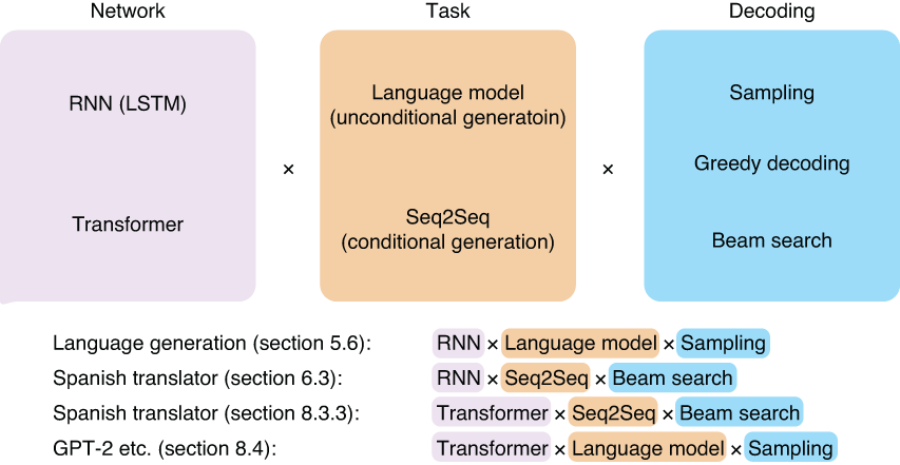
Figure 8.14 Three components of language generation and Seq2Seq tasks
In the rest of this section, we are going to experiment with some Transformer-based language models and generate natural language texts using them. We’ll be using the transformers library (https://huggingface.co/transformers/) developed by Hugging Face, which has become a standard, go-to library for NLP researchers and engineers working with Transformer models in the past few years. It comes with a number of state-of-the-art model implementations including GPT-2 (this section) and BERT (next chapter), along with pretrained model parameters that you can load and use right away. It also provides a simple, consistent interface through which you can interact with powerful NLP models.
8.4.2 Transformer-XL
In many cases, you want to load and use pretrained models provided by third parties (most often the developer of the model), instead of training them from scratch. Recent Transformer models are fairly complex (usually with hundreds of millions of parameters) and are trained with huge datasets (tens of gigabytes of text). This would require GPU resources that only large institutions and tech giants can afford. It is not completely uncommon that some of these models take days to train, even with more than a dozen GPUs! The good news is the implementation and pretrained model parameters for these huge Transformer models are usually made publicly available by their creators so that anyone can integrate them into their NLP applications.
In this section, we’ll first check out Transformer-XL, a variant of the Transformer developed by the researchers at Google Brain. Because there is no inherent “loop” in the original Transformer model, unlike RNNs, the original Transformer is not good at dealing with super-long context. In training language models with the Transformer, you first split long texts into shorter chunks of, say, 512 words, and feed them to the model separately. This means the model is unable to capture dependencies longer than 512 words. Transformer-XL4 addresses this issue by making a few improvements over the vanilla Transformer model (“XL” means extra-long). Although the details of these changes are outside the scope of this book, in a nutshell, the model reuses its hidden states from the previous segment, effectively creating a loop that passes information between different segments of texts. It also improves the positional encoding scheme we touched on earlier to make it easier for the model to deal with longer texts.
You can install the transformers library just by running pip install transformers from the command line. The main abstractions you’ll be interacting with are tokenizers and models. The tokenizers split a raw string into a sequence of tokens, whereas the model defines the architecture and implements the main logic. The model and the pretrained weights usually depend on a specific tokenization scheme, so you need to make sure you are using the tokenizer that is compatible with the model.
The easiest way to initialize a tokenizer and a model with some specified pretrained weights is use the AutoTokenizer and AutoModelWithLMHead classes and call their from_pretrained() methods as follows:
import torch
from transformers import AutoModelWithLMHead, AutoTokenizer

tokenizer = AutoTokenizer.from_pretrained('transfo-xl-wt103')
model = AutoModelWithLMHead.from_pretrained('transfo-xl-wt103')
The parameter to from_pre-trained() is the name of the model/pretrained weights. This is a Transformer-XL model trained on a dataset called wt103 (WikiText103).
You may be wondering what this “LMHead” part in AutoModelWithLMHead means. An LM (language model) head is a specific layer added to a neural network that converts its hidden states to a set of scores that determine which tokens to generate next. These scores (also called logits) are then fed to a softmax layer to obtain a probability distribution over possible next tokens (figure 8.15). We would like a model with an LM head because we are interested in generating text by using the Transformer as a language model. However, depending on the task, you may also want a Transformer model without an LM head and just want to use its hidden states. That’s what we’ll do in the next chapter.
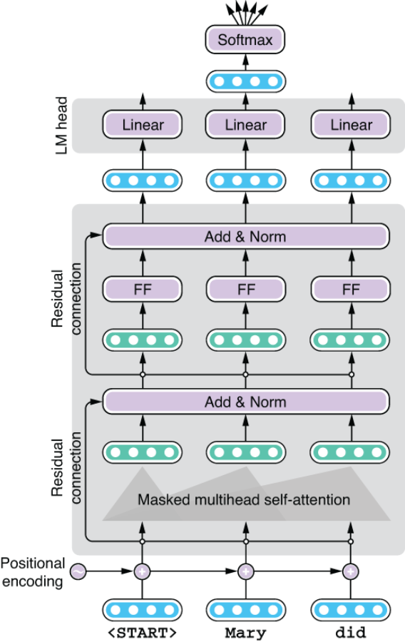
Figure 8.15 Using a language model head with the Transformer
The next step is to initialize the prefix for which you would like your language model to write the rest of the story. You can use tokenizer.encode() to convert a string into a list of token IDs, which are then converted to a tensor. We’ll also initialize a variable past for caching the internal states and making the inference faster, as shown next:
generated = tokenizer.encode("On our way to the beach")
context = torch.tensor([generated])
past = None
Now you are ready to generate the rest of the text. Notice the next code is similar to the pseudocode we showed earlier. The idea is simple: get the output from the model, sample a token using the output, and feed it back to the model. Rinse and repeat.
for i in range(100):
    output = model(context, mems=past)
    token = sample_token(output.prediction_scores)

    generated.append(token.item())
    context = token.view(1, -1)
    past = output.mems
You need to do some housekeeping to make the shape of the tensors compatible with the model, which we can ignore for now. The sample_token() method here takes the output of the model, converts it to a probability distribution, and samples a single token from it. I’m not showing the entire code for the method, but you can check the Google Colab notebook (http://realworldnlpbook.com/ch8.html#xformer-nb) for more details. Also, here we wrote the generation algorithm from scratch, but if you need more full-fledged generation (such as beam search), check out the official example script from the developers of the library: http://mng.bz/wQ6q.
After finishing the generation, you can convert the token IDs back into a raw string by calling tokenizer.decode()as follows:
print(tokenizer.decode(generated))
The following “story” is what I got when I ran this:
On our way to the beach, she finds, she finds the men who are in the group to be " in the group ". This has led to the perception that the " group " in the group is " a group of people in the group with whom we share a deep friendship, and which is a common cause to the contrary. " <eos> <eos> = = Background = = <eos> <eos> The origins of the concept of " group " were in early colonial years with the English Civil War. The term was coined by English abolitionist John
This is not a bad start. I like the way the story is trying to be consistent by sticking with the concept of “group.” However, because the model is trained on Wikipedia text only, its generation is not realistic and looks a little bit too formal.
8.4.3 GPT-2
GPT-2 (which stands for generative pretraining), developed by OpenAI, is probably the most famous language model to date. You may have heard the story about a language model generating natural language texts that are so realistic that you cannot tell them from those written by humans. Technically, GPT-2 is just a huge Transformer model, just like the one we introduced earlier. The main difference is its size (the largest model has 48 layers!) and the fact that the model is trained on a huge amount of natural language text collected from the web. The OpenAI team publicly released the implementation and the pretrained weights, so we can easily try out the model.
Initialize the tokenizer and the model for GPT-2 as you have done for Transformer-XL, as shown next:
tokenizer = AutoTokenizer.from_pretrained('gpt2-large')
model = AutoModelWithLMHead.from_pretrained('gpt2-large')
Then generate text using the next code snippet:
generated = tokenizer.encode("On our way to the beach")
context = torch.tensor([generated])
past = None

for i in range(100):
    output = model(context, past_key_values=past)
    token = sample_token(output.logits)

    generated.append(token.item())
    context = token.unsqueeze(0)
    past = output.past_key_values

print(tokenizer.decode(generated))
You may have noticed how little this code snippet changed from the one for Transformer-XL. In many cases, you don’t need to make any modifications when switching between different models. This is why the transformers library is so powerful—you can try out and integrate a variety of state-of-the-art Transformer-based models into your application with a simple, consistent interface. As we’ll see in the next chapter, this library is also integrated into AllenNLP, which makes it easy to build powerful NLP applications with state-of-the-art models.
When I tried this, the GPT-2 generated the following beautifully written passage:
On our way to the beach, there was a small island that we visited for the first time. The island was called 'A' and it is a place that was used by the French military during the Napoleonic wars and it is located in the south-central area of the island.

A is an island of only a few hundred meters wide and has no other features to distinguish its nature. On the island there were numerous small beaches on which we could walk. The beach of 'A' was located in the...
Notice how naturally it reads. Also, the GPT-2 model is good at staying consistent—you can see the name of the island, “A,” is consistently used throughout the passage. As far as I checked, there is no real island named A in the world, meaning that this is something the model simply made up. It is a great feat that the model remembered the name it just coined and successfully wrote a story around it!
Here’s another passage that GPT-2 generated with a prompt: 'Real World Natural Language Processing' is the name of the book:
'Real World Natural Language Processing' is the name of the book. It has all the tools you need to write and program natural language processing programs on your computer. It is an ideal introductory resource for anyone wanting to learn more about natural language processing. You can buy it as a paperback (US$12), as a PDF (US$15) or as an e-book (US$9.99).

The author's blog has more information and reviews.

The free 'Real World Natural Language Processing' ebook has all the necessary tools to get started with natural language processing. It includes a number of exercises to help you get your feet wet with writing and programming your own natural language processing programs, and it includes a few example programs. The book's author, Michael Karp has also written an online course about Natural Language Processing.

'Real World Natural Language Processing: Practical Applications' is a free e-book that explains how to use natural language processing to solve problems of everyday life (such as writing an email, creating and
As of February 2019, when GPT-2 was released, I had barely begun writing this book, so I doubt GPT-2 knew anything about it. For a language model that doesn’t have any prior knowledge about the book, this is an amazing job, although I have to note that it got the price and the name of the author wrong.
8.4.4 XLM
Finally, as an interesting example, we will experiment with multilingual language generation. XLM (cross-lingual language model), proposed by researchers at Facebook AI Research, is a Transformer-based cross-lingual language model that can generate and encode texts in multiple languages.5 By learning how to encode multilingual texts, the model can be used for transfer learning between different languages. We’ll cover transfer learning in chapter 9.
You can start by initializing the tokenizer and the model and initialize it with the pretrained weights as follows:
tokenizer = AutoTokenizer.from_pretrained('xlm-clm-enfr-1024')
model = AutoModelWithLMHead.from_pretrained('xlm-clm-enfr-1024')
Here, we are loading an XLM model (xlm), trained with a causal language modeling (CLM) objective (clm) in English and French (enfr). CLM is just a fancier way to describe what we’ve been doing in this chapter—predicting the next token based on a prefix. XLM is usually used for encoding multilingual texts for some downstream tasks such as text classification and machine translation, but we are simply using it as a language model to generate texts. See listing 8.2 for the code snippet for generating multilingual text with XLM. You can again reuse most of the earlier code snippet, although you also need to specify what language you are working in (note the lang = 0 line). Also, here we are generating text from scratch by supplying just the BOS token (whose index is zero).
Listing 8.2 Generating multilingual text with XLM
generated = [0] # start with just <s>
context = torch.tensor([generated])
lang = 0 # English

for i in range(100):
    langs = torch.zeros_like(context).fill_(lang)
    output = model(context, langs=langs)
    token = sample_token(output)

    generated.append(token.item())
    context = torch.tensor([generated])

print(tokenizer.decode(generated))
When I ran this, I got the following:
<s>and its ability to make decisions on the basis of its own. " </s>The government has taken no decisions on that matter, " Mr Hockey said. </s>A lot of the information is very sensitive. </s>The new research and information on the Australian economy, which is what we're going to get from people, and the information that we are going to be looking at, we're going to be able to provide and we 'll take it forward. </s>I'm not trying to make sure we're not
Then, let’s change lang to 1 (which means French) and run the same snippet again, which gives you the next bit of text:
<s></s>En revanche, les prix des maisons individuelles n' ont guère augmenté ( - 0,1 % ). </s>En mars dernier, le taux de la taxe foncière, en légère augmentation à la hausse par rapport à février 2008. </s>" Je n' ai jamais eu une augmentation " précise ". </s>" Je me suis toujours dit que ce n' était pas parce que c' était une blague. </s>En effet, j' étais un gars de la rue " </s>Les jeunes sont des gens qui avaient beaucoup d' humour... "
Although the quality of generation is not as great as GPT-2, which we experimented with earlier, it is refreshing to see that a single model can produce texts both in English and French. These days, it is increasingly common to build multilingual Transformer-based NLP models to solve NLP problems and tasks in multiple languages at the same time. This also became possible thanks to the Transformer’s powerful capacity to model the complexity of language.
8.5 Case study: Spell-checker
In the final section of this chapter, we will build a practical NLP application—a spell-checker—with the Transformer. In the modern world, spell-checkers are everywhere. Chances are your web browser is equipped with a spell-checker that tells you when you make a spelling mistake by underlining misspelled words. Many word processors and editors also run spell-checkers by default. Some applications (including Google Docs and Microsoft Word) even point out simple grammatical errors, too. Ever wondered how they work? We’ll learn how to formulate this as an NLP problem, prepare the dataset, train, and improve the model next.
8.5.1 Spell correction as machine translation
Spell-checkers receive a piece of text such as “tisimptant too spll chck ths dcment,” detect spelling and grammatical errors, if any, and fix all errors: “It’s important to spell-check this document.” How can you solve this task with NLP technologies? How can such systems be implemented?
The simplest thing you could do is tokenize the input text into words and check if each word is in a dictionary. If it’s not, you look for the closest valid word in the dictionary according to some measure such as the edit distance and replace with that word. You repeat this until there are no words to fix. This word-by-word fixing algorithm is widely used by many spell-checkers due to its simplicity.
However, this type of spell-checker has several issues. First, just like the first word in the example, “tisimptant,” how do you know which part of the sentence is actually a word? The default spell-checker for my copy of Microsoft Word indicates it’s a misspelling of “disputant,” although it would be obvious to any English speakers that it is actually a misspelling of two (or more) words. The fact that users can also misspell punctuation (including whitespace) makes everything complicated. Second, just because some word is in a dictionary doesn’t mean it’s not an error. For example, the second word in the example, “too” is a misspelling of “to,” but both are valid words that are in any English dictionary. How can you tell if the former is wrong in this context? Third, all these decisions are made out of context. One of the spell-checkers I tried shows “thus” as a candidate to replace “ths” in this example. However, from this context (before a noun), it is obvious that “this” is a more appropriate candidate, although both “this” and “thus” are one edit distance away from “ths,” meaning they are equally valid options according to the edit distance.
You would be able to solve some of these issues by adding some heuristic rules. For example, “too” is more likely a misspelling of “to” before a verb, and “this” is more likely before a noun than “thus.” But this method is obviously not scalable. Remember the poor junior developer from section 1.1.2? Language is vast and full of exceptions. You cannot just keep writing such rules to deal with the full complexity of language. Even if you are able to write rules for such simple words, how would you tell that “tisimptant” is actually two words? Would you try to split this word at every possible position to see if split words resemble existing words? What if the input was in a language that is written without whitespace, like Chinese and Japanese?
At this point, you may realize this “split and fix” approach is going nowhere. In general, when designing an NLP application, you should think in terms of the following three aspects:
-
Task—What is the task being solved? Is it a classification, sequential-labeling, or sequence-to-sequence problem?
-
Model—What model are you going to use? Is it a feed-forward network, an RNN, or the Transformer?
-
Dataset—Where are you obtaining the dataset to train and validate your model?
Based on my experience, a vast majority of NLP applications nowadays can be solved by combining these aspects. How about spell-checkers? Because they take a piece of text as the input and produce the fixed string, it’d be most straightforward if we solve this as a Seq2Seq task using the Transformer model. In other words, we will be building a machine translation system that translates noisy inputs with spelling/grammatical errors into clean, errorless outputs as shown in figure 8.16. You can regard these two sides as two different “languages” (or “dialects” of English).
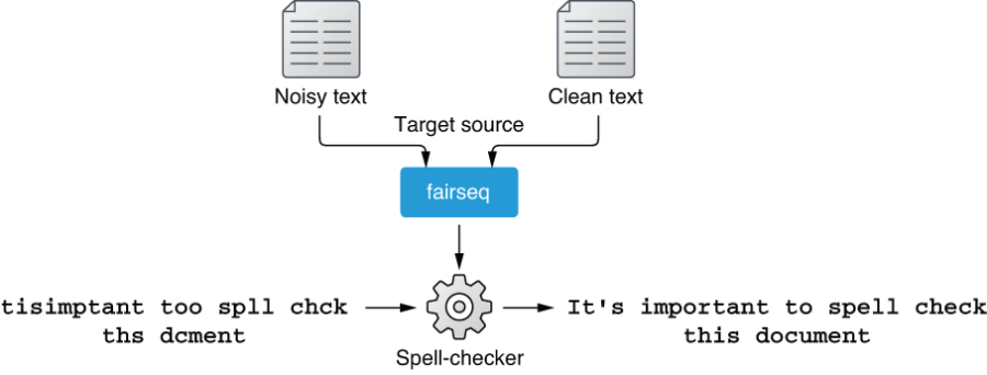
Figure 8.16 Training a spell-checker as an MT system that translates “noisy” sentences into “clean” ones
At this point, you may be wondering where we are obtaining the dataset. This is often the most important (and the most difficult) part in solving real-world NLP problems. Fortunately, we can use a public dataset for this task. Let’s dive in and start building a spell-checker.
8.5.2 Training a spell-checker
We will be using GitHub Typo Corpus (https://github.com/mhagiwara/github-typo -corpus) as the dataset to train a spell-checker. The dataset, created by my collaborator and me, consists of hundreds of thousands of “typo” edits automatically harvested from GitHub. It is the largest dataset of spelling mistakes and their corrections to date, which makes it a perfect choice for training a spell-checker.
One decision we need to make before preparing the dataset and training a model is what to use as the atomic linguistic unit on which the model operates. Many NLP models use tokens as the smallest unit (i.e., RNN/Transformer is fed a sequence of tokens), but a growing number of NLP models use word or sentence pieces as the basic units (section 10.4). What should we use as the smallest unit for spelling correction? As with many other NLP models, using words as the input sounds like a good “default” thing to do at first. However, as we saw earlier, the concept of tokens is not well suited for spelling correction—users can mess up with punctuation, which makes everything overly complex if you are dealing with tokens. More importantly, because NLP models need to operate on a fixed vocabulary, the spell-corrector vocabulary would need to include every single misspelling of every single word it encountered during the training. This would make it unnecessarily expensive to train and maintain such an NLP model.
For these reasons, we will be using characters as the basic unit for our spell-checker, as we did in section 5.6. Using characters has several advantages—it can keep the size of the vocabulary quite small (usually less than one hundred for a language with a small set of alphabets such as English). You don’t need to worry about bloating your vocabulary, even with a noisy dataset full of typos, because typos are just different arrangements of characters. You can also treat punctuation marks (even whitespace) as one of the characters in the vocabulary. This makes the preprocessing step extremely easy because you don’t need any linguistic toolkits (such as tokenizers) for doing this.
NOTE Using characters is not without disadvantages. One main issue is using them will increase the length of sequences, because you need to break everything up into characters. This makes the model large and slower to train.
First, let’s prepare the dataset for training a spell-checker. All the necessary data and code for building a spell-checker are included in this repository: https://github.com/mhagiwara/xfspell. The tokenized and split datasets are located under data/gtc (as train.tok.fr, train.tok.en, dev.tok.fr, dev.tok.en). The suffixes en and fr are a commonly used convention in machine translation—“fr” means “foreign language” and “en” means English, because many MT research projects were originally motivated by people wanting to translate some foreign language into English. Here, we are using “fr” and “en” to mean just “noisy text before spelling correction” and “clean text after spelling correction.”
Figure 8.17 shows an excerpt from the dataset for spelling correction created from GitHub Typo Corpus. Notice that text is segmented into individual characters, even whitespaces (replaced by “_”). Any characters outside common alphabets (upper- and lowercase letters, numbers, and some common punctuation marks) are replaced with “#.” You can see that the dataset contains diverse corrections, including simple typos (pubilc -> public on line 670, HYML -> HTML on line 672), trickier errors (mxnet as not -> mxnet is not on line 681, 22th -> 22nd on line 682), and even lines without any corrections (line 676). This looks like a good resource to use for training a spell-checker.
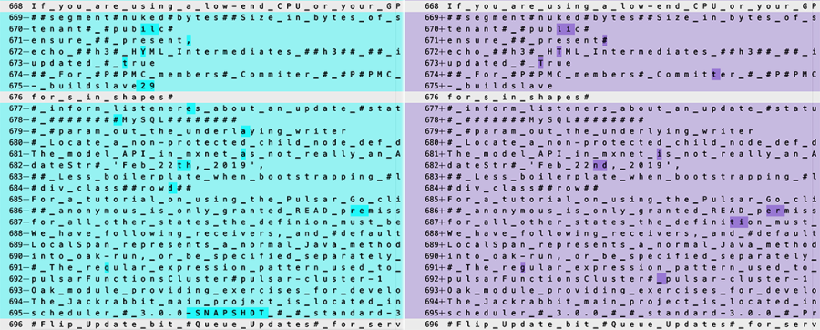
Figure 8.17 Training data for spelling correction
The first step for training a spell-checker (or any other Seq2Seq model) is to preprocess the datasets. Because the dataset is already split and formatted, all you need to do is run fairseq-preprocess to convert the datasets into a binary format as follows:
fairseq-preprocess --source-lang fr --target-lang en
    --trainpref data/gtc/train.tok
    --validpref data/gtc/dev.tok
    --destdir bin/gtc
Then you can start training your model right away using the following code.
Listing 8.3 Training a spell-checker
fairseq-train
    bin/gtc
    --fp16
    --arch transformer
    --encoder-layers 6 --decoder-layers 6
    --encoder-embed-dim 1024 --decoder-embed-dim 1024
    --encoder-ffn-embed-dim 4096 --decoder-ffn-embed-dim 4096
    --encoder-attention-heads 16 --decoder-attention-heads 16
    --share-decoder-input-output-embed
    --optimizer adam --adam-betas '(0.9, 0.997)' --adam-eps 1e-09 --clip-norm 25.0
    --lr 1e-4 --lr-scheduler inverse_sqrt --warmup-updates 16000
    --dropout 0.1 --attention-dropout 0.1 --activation-dropout 0.1
    --weight-decay 0.00025
    --criterion label_smoothed_cross_entropy --label-smoothing 0.2
    --max-tokens 4096
    --save-dir models/gtc01
    --max-epoch 40
You don’t need to worry about most of the hyperparameters here—this set of parameters worked fairly well for me, although some other combinations of parameters may work better. However, you may want to pay attention to some of the parameters related to the size of the model, namely:
-
Embedding dimension of self-attention (—[encoder|decoder]-embed-dim)
-
Embedding dimension of feed-forward layers (—[encoder/decoder]-ffn-embed-dim)
-
Number of attention heads (—[encoder|decoder]-attention-heads)
These parameters determine the capacity of the model. In general, the larger these parameters are, the larger capacity the model would have, although as a result the model would also require more data, time, and GPU resources to train. Another important parameter is —max-tokens, which specifies the number of tokens loaded onto a single batch. If you are experiencing out-of-memory errors on a GPU, try adjusting this parameter.
After the training is finished, you can run the following command to make predictions using the trained model:
echo "tisimptant too spll chck ths dcment."
    | python src/tokenize.py
    | fairseq-interactive bin/gtc
    --path models/gtc01/checkpoint_best.pt
    --source-lang fr --target-lang en --beam 10
    | python src/format_fairseq_output.py
Because the fairseq-interactive interface can also take source text from the standard input, we are directly providing the text using the echo command. The Python script src/format_fairseq_output.py, as its name suggests, formats the output from fairseq-interactive and shows the predicted target text. When I ran this, I got the following:
tisimplement too spll chck ths dcment.
This is rather disappointing. The spell-checker learned to somehow fix “imptant” to “implement,” although it failed to correct any other words. I suspect a couple of reasons for this. The training data used, GitHub Typo Corpus, is heavily biased toward software-related language and corrections, which might have led to the wrong correction (imptant -> implement). Also, the training data might have just been too small for the Transformer to be effective. How could we improve the model so that it can fix spellings more accurately?
8.5.3 Improving a spell-checker
As we discussed earlier, one main reason the spell-checker is not working as expected might be because the model wasn’t exposed to a more diverse, larger amount of misspellings during training. But as far as I know, no such large datasets of diverse misspellings are publicly available for training a general-domain spell-checker. How could we obtain more data for training a better spell-checker?
This is where we need to be creative. One idea is to artificially generate noisy text from clean text. If you think of it, it is very difficult (especially for a machine learning model) to fix misspellings, whereas it is very easy to “corrupt” clean text to simulate how people make typos, even for a computer. For example, we can take some clean text (which is available from, for example, scraped web text almost indefinitely) and replace some letters at random. If you pair artificially generated noisy text created this way with the original, clean text, this will effectively create a new, larger dataset on which you can train an even better spell-checker!
The remaining issue we need to address is how to “corrupt” clean text to generate realistic spelling errors that look like the ones made by humans. You can write a Python script that, for example, replaces, deletes, and/or swaps letters at random, although there is no guarantee that typos made this way are similar to those made by humans and that the resulting artificial dataset will provide useful insights for the Transformer model. How can we model the fact that, for example, humans are more likely to type “too” in place of “to” than they do “two”?
This is starting to sound familiar again. We can use the data to simulate the typos! But how? This is where we need to be creative again—if you “flip” the direction of the original dataset we used to train the spell-checker, you can observe how humans make typos. If you treat the clean text as the source language and the noisy text as the target and train a Seq2Seq model for that direction, you are effectively training a “spell-corruptor”—a Seq2Seq model that inserts realistic-looking spelling errors into clean text. See Figure 8.18 for an illustration.

Figure 8.18 Using back-translation to generate artificial noisy data
This technique of using the “inverse” of the original training data to artificially generate a large amount of data in the source language from a real corpus in the target language is called back-translation in the machine learning literature. It is a popular technique to improve the quality of machine translation systems. As we’ll show next, it is also effective for improving the quality of spell-checkers.
You can easily train a spell corruptor just by swapping the source and the target languages. You can do this by supplying “en” (clean text) as the source language and “fr” (noisy text) as the target language when you run fairseq-preprocess as follows:
fairseq-preprocess --source-lang en --target-lang fr
    --trainpref data/gtc/train.tok
    --validpref data/gtc/dev.tok
    --destdir bin/gtc-en2fr
We are not going over the training process again—you can use almost the same fairseq-train command to start the training. Just don’t forget to specify a different directory for —save-dir. After you finish training, you can check whether the spelling corrupter can indeed corrupt the input text as expected:
$ echo 'The quick brown fox jumps over the lazy dog.' | python src/tokenize.py
    | fairseq-interactive
    bin/gtc-en2fr
    --path models/gtc-en2fr/checkpoint_best.pt
    --source-lang en --target-lang fr
    --beam 1 --sampling --sampling-topk 10
    | python src/format_fairseq_output.py
The quink brown fox jumps ove-rthe lazy dog.
Note the extra options that I added earlier, which are shown in bold. It means that the fairseq-interactive command uses sampling (from top 10 tokens with largest probabilities) instead of beam search. When corrupting clean text, it is often better to use sampling instead of beam search. To recap, sampling picks the next token randomly according to the probability distribution after the softmax layer, whereas beam search tries to find the “best path” that maximizes the score of the output sequence. Although beam search can find better solutions when translating some text, we want noisy, more diverse output when corrupting clean text. Past research6 has also shown that sampling (instead of beam search) works better for augmenting data via back-translation.
From here, the sky’s the limit. You can collect as much clean text as you want, generate noisy text from it using the corruptor you just trained, and increase the size of the training data. There is no guarantee that the artificial errors look like the real ones made by humans, but this is not a big deal because 1) the source (noisy) side is used only for encoding, and 2) the target (clean) side data is always “real” data written by humans, from which the Transformer can learn how to generate real text. The more text data you collect, the more confident the model will get about what error-free, real text looks like.
I won’t go over every step I took to increase the size of the data, but here’s the summary of what I did and what you can also do. Collect as much clean and diverse text data from publicly available datasets, such as Tatoeba and Wikipedia dumps. My favorite way to do this is to use OpenWebTextCorpus (https://skylion007.github.io/OpenWebTextCorpus/), an open source project to replicate the dataset on which GPT-2 was originally trained. It consists of a huge amount (40 GB) of high-quality web text crawled from all outbound links from Reddit. Because the entire dataset would take days, if not weeks, just to preprocess and run the corruptor on, you can take a subset (say, 1/1000th) and add it to the dataset. I took 1/100th of the dataset, preprocessed it, and ran the corruptor to obtain the noisy-clean parallel dataset. This 1/100th subset alone added more than five million pairs (in comparison, the original training set contains only ~240k pairs). Instead of training from scratch, you can download the pretrained weights and try the spell-checker from the repository.
The training took several days, even on multiple GPUs, but when it was done, the result was very encouraging. Not only can it accurately fix spelling errors, as shown here
$ echo "tisimptant too spll chck ths dcment."
    | python src/tokenize.py
    | fairseq-interactive
    bin/gtc-bt512-owt1k-upper
    --path models/bt05/checkpoint_best.pt
    --source-lang fr --target-lang en --beam 10
    | python src/format_fairseq_output.py
    It's important to spell check this document.
but the spell-checker also appears to understand the grammar of English to some degree, as shown here:
$ echo "The book wer about NLP." |
    | python src/tokenize.py
    | fairseq-interactive
   ...
The book was about NLP.

$ echo "The books wer about NLP." |
    | python src/tokenize.py
    | fairseq-interactive
   ...
The books were about NLP.
This example alone may not prove that the model really understands the grammar (namely, using the correct verb depending on the number of the subject). It might just be learning some association between consecutive words, which can be achieved by any statistical NLP model, such as n-gram language models. However, even after you make the sentences more complicated, the spell-checker shows amazing resilience, as shown in the next code snippet:
$ echo "The book Tom and Jerry put on the yellow desk yesterday wer about NLP." |
    | python src/tokenize.py
    | fairseq-interactive
   ...
The book Tom and Jerry put on the yellow desk yesterday was about NLP.

$ echo "The books Tom and Jerry put on the yellow desk yesterday wer about NLP." |
    | python src/tokenize.py
    | fairseq-interactive
   ...
The books Tom and Jerry put on the yellow desk yesterday were about NLP.
From these examples, it is clear that the model learned how to ignore irrelevant noun phrases (such as “Tom and Jerry” and “yellow desk”) and focus on the noun (“book(s)”) that determines the form of the verb (“was” versus “were”). We are more confident that it understands the basic sentence structure. All we did was collect a large amount of clean text and trained the Transformer model on it, combined with the original training data and the corruptor. Hopefully through these experiments, you were able to feel how powerful the Transformer model can be!
Summary
-
Attention is a mechanism in neural networks that focuses on a specific part of the input and computes its context-dependent summary. It works like a “soft” version of a key-value store.
-
Encoder-decoder attention can be added to Seq2Seq models to improve their translation quality.
-
Self-attention is an attention mechanism that produces the summary of the input by summarizing itself.
-
The Transformer model applies self-attention repeatedly to gradually transform the input.
-
High-quality spell-checkers can be built using the Transformer and a technique called back-translation.