3 Word and document embeddings

This chapter covers

• What word embeddings are and why they are important
• How the Skip-gram model learns word embeddings and how to implement it
• What GloVe embeddings are and how to use pretrained vectors
• How to use Doc2Vec and fastText to train more advanced embeddings
• How to visualize word embeddings

In chapter 2, I pointed out that neural networks can deal only with numbers, whereas almost everything in natural language is discrete (i.e., separate concepts). To use neural networks in your NLP application, you need to convert linguistic units to numbers, such as vectors. For example, if you wish to build a sentiment analyzer, you need to convert the input sentence (sequence of words) into a sequence of vectors. In this chapter, we’ll discuss word embeddings, which are the key to achieving this bridging. We’ll also touch upon a couple of fundamental linguistic components that are important in understanding embeddings and neural networks in general.

3.1 Introducing embeddings

As we discussed in chapter 2, an embedding is a real-valued vector representation of something that is usually discrete. In this section, we’ll revisit what embeddings are and discuss in detail what roles they play in NLP applications.

3.1.1 What are embeddings?

A word embedding is a real-valued vector representation of a word. If you find the concept of vectors intimidating, think of them as single-dimensional arrays of float numbers, like the following:

• vec("cat") = [0.7, 0.5, 0.1]

• vec("dog") = [0.8, 0.3, 0.1]

• vec("pizza") = [0.1, 0.2, 0.8]

Because each array contains three elements, you can plot them as points in a 3-D space as in figure 3.1. Notice that semantically-related words (“cat” and “dog”) are placed close to each other.

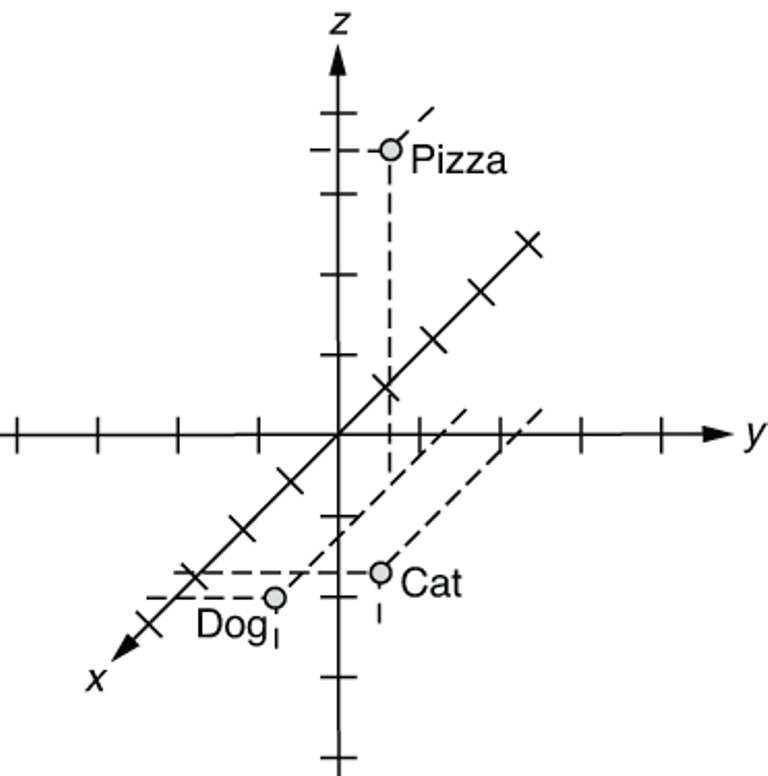
Figure 3.1 Word embeddings on a 3-D space

NOTE In fact, you can embed (i.e., represent by a list of numbers) not just words but also almost anything—characters, sequences of characters, sentences, or categories. You can embed any categorical variables using the same method, although in this chapter, we’ll focus on two of the most important concepts in NLP—words and sentences.

3.1.2 Why are embeddings important?

Why are embeddings important? Well, word embeddings are not just important but essential for using neural networks to solve NLP tasks. Neural networks are pure mathematical computation models that can deal only with numbers. They can’t do symbolic operations, such as concatenating two strings or conjugating a verb to past tense, unless these items are all represented by numbers and arithmetic operations. On the other hand, almost everything in NLP, such as words and labels, is symbolic and discrete. This is why you need to bridge these two worlds, and using embeddings is a way to do it. See figure 3.2 for an overview on how to use word embeddings for an NLP application.

Figure 3.2 Using word embeddings with NLP models

Word embeddings, just like any other neural network models, can be trained, because they are simply a collection of parameters (or “magic constants,” which we talked about in the previous chapter). Embeddings are used with your NLP model in the following three scenarios:

• Scenario 1: Train word embeddings and your model at the same time using the train set for your task.

• Scenario 2: First, train word embeddings independently using a larger text dataset. Alternatively, obtain pretrained word embeddings from somewhere else. Then initialize your model using the pretrained word embeddings, and train them and your model at the same time using the train set for your task.

• Scenario 3: Same as scenario 2, except you fix word embeddings while you train your model.

In the first scenario, word embeddings are initialized randomly and trained in conjunction with your NLP model using the same dataset. This is basically how we built the sentiment analyzer in chapter 2. Using an analogy, this is like having a dance teacher teach a baby to walk and dance at the same time. It is not an entirely impossible feat (in fact, some babies might end up being better, maybe more creative dancers by skipping the walking part, but don’t try this at home), but rarely a good idea. Babies would probably have a much better chance if they are taught how to stand and walk properly first, and then how to dance.

Similarly, it’s not uncommon to train an NLP model and word embeddings as its subcomponent at the same time. But many large-scale, high-performance NLP models usually rely on external word embeddings that are pretrained using larger datasets (scenarios 2 and 3). Word embeddings can be learned from unlabeled large text datasets—that is, a large amount of plain text data (e.g., Wikipedia dumps), which are usually more readily available than the train datasets for your task (e.g., the Stanford Sentiment Treebank). By leveraging such large textual data, you can teach your model a lot about how natural language works even before it sees a single instance from the dataset for your task. Training a machine learning model on one task and repurposing it for another task is called transfer learning, which is becoming increasingly popular in many machine learning domains, NLP included. We’ll further discuss transfer learning in chapter 9.

Using the dancing baby analogy again, most healthy babies figure out how to stand and walk themselves. They may get some help from adults, usually from their close caregivers such as parents. This form of “help,” however, is usually a lot more abundant and cheaper than the “training signal” you get from a hired dance teacher, which is why it’s a lot more effective if they learn how to walk first, then move on to dancing. Many skills used for walking transfer to dancing.

The difference between scenarios 2 and 3 is whether the word embeddings are adjusted, or fine-tuned, while your NLP model is trained. Whether or not this is effective may depend on your task and the dataset. Teaching your toddler ballet may have a good effect on how they walk (e.g., by improving their posture), which in turn could have a positive effect on how they dance, but scenario 3 doesn’t allow this to happen.

The only remaining question you might have is: Where do embeddings come from? I mentioned earlier that they can be trained from a large amount of plain text. This chapter explains how this is possible and what models are used to achieve this.

3.2 Building blocks of language: Characters, words, and phrases

Before I explain word-embedding models, I’m going to touch upon some basic concepts of language, such as characters, words, and phrases. It helps to understand these concepts when you design the structure of your NLP application. Figure 3.3 shows some examples of those concepts.

3.2.1 Characters

A character (also called a grapheme in linguistics) is the smallest unit of a writing system. In written English, “a,” “b,” and “z” are characters. Characters do not necessarily carry meaning by themselves or represent any fixed sound when spoken, although in some languages (e.g., Chinese), most do. A typical character in many languages can be represented by a single Unicode codepoint (by string literals such as "uXXXX" in Python), but this is not always the case. Many languages use a combination of more than one Unicode codepoint (e.g., accent marks) to represent a single character. Punctuation marks, such as “.” (period), “,” (comma), and “?” (question mark), are also characters.

Figure 3.3 Building blocks of language used in NLP

3.2.2 Words, tokens, morphemes, and phrases

A word is the smallest unit in a language that can be uttered independently and that usually carries some meaning. In English, “apple,” “banana,” and “zebra” are words. In most written languages that use alphabetic scripts, words are usually separated by spaces or punctuation marks. In some languages, like Chinese, Japanese, and Thai, however, words are not explicitly delimited by spaces and require a preprocessing step called word segmentation to identify words in a sentence.

A closely related concept to a word in NLP is a token. A token is a string of contiguous characters that play a certain role in a written language. Most words (“apple,” “banana,” “zebra”) are also tokens when written. Punctuation marks such as the exclamation mark (“!”) are tokens but not words, because you can’t utter them in isolation. Word and token are often used interchangeably in NLP. In fact, when you see “word” in NLP text (including this book), it often means “token,” because most NLP tasks deal only with written text that is processed in an automatic way. Tokens are the output of a process called tokenization, which I’ll explain more below.

Another closely related concept is morpheme. A morpheme is the smallest unit of meaning in a language. A typical word consists of one or more morphemes. For example, “apple” is a word and also a morpheme. “Apples” is a word comprised of two morphemes, “apple” and “-s,” which is used to signify the noun is plural. English contains many other morphemes, including “-ing,” “-ly,” “-ness,” and “un-.” The process for identifying morphemes in a word or a sentence is called morphological analysis, and it has a wide range of NLP/linguistics applications, but this is outside the scope of this book.

A phrase is a group of words that play a certain grammatical role. For example, “the quick brown fox” is a noun phrase (a group of words that behaves like a noun), whereas “jumps over the lazy dog” is a verb phrase. The concept of phrase may be used somewhat liberally in NLP to simply mean any group of words. For example, in many NLP literatures and tasks, words like “Los Angeles” are treated as phrases, although, linguistically speaking, they are closer to a word.

3.2.3 N-grams

Finally, you may encounter the concept of n-grams in NLP. An n-gram is a contiguous sequence of one or more occurrences of linguistic units, such as characters and words. For example, a word n-gram is a contiguous sequence of words, such as “the” (one word), “quick brown” (two words), “brown fox jumps” (three words). Similarly, a character n-gram is composed of characters, such as “b” (one character), “br” (two characters), “row” (three characters), and so on, which are all character n-grams made from “brown.” An n-gram of size 1 (when n = 1) is called a unigram. N-grams of size 2 and 3 are called a bigram and a trigram, respectively.

Word n-grams are often used as proxies for phrases in NLP, because if you enumerate all the n-grams of a sentence, they often contain linguistically interesting units that correspond to phrases such as “Los Angeles” and “take off.” In a similar vein, we use character n-grams when we want to capture subword units that roughly correspond to morphemes. In NLP, when you see “n-grams” (without a qualifier), they are often word n-grams.

NOTE Interestingly, in search and information retrieval, n-grams often mean character n-grams used for indexing documents. Be mindful which type of n-grams are implied by the context when you read papers.

3.3 Tokenization, stemming, and lemmatization

We covered some basic linguistic units often encountered in NLP. In this section, I introduce some steps where linguistic units are processed in a typical NLP pipeline.

3.3.1 Tokenization

Tokenization is a process where the input text is split into smaller units. There are two types of tokenization: word and sentence tokenization. Word tokenization splits a sentence into tokens (rough equivalent to words and punctuation), which I mentioned earlier. Sentence tokenization, on the other hand, splits a piece of text that may include more than one sentence into individual sentences. If you say tokenization, it usually means word tokenization in NLP.

Many NLP libraries and frameworks support tokenization out of the box, because it is one of the most fundamental and widely used preprocessing steps in NLP. In what follows, I show you how to do tokenization using two popular NLP libraries—NLTK (https://www.nltk.org/) and spaCy (https://spacy.io/).

NOTE Before running the example code in this section, make sure the libraries are both installed. In a typical Python environment, they can be installed by running pip install nltk and pip install spacy. After installation, you need to download the necessary data and models by running python -c "import nltk; nltk.download('punkt')" for NLTK, and python -m spacy download en for spaCy from the command line. You can also run all the examples in this section via Google Colab (http://realworldnlpbook.com/ch3.html#tokeni zation) without installing any Python environments or dependencies.

To use the default word and sentence tokenizers from NLTK, you can import them from nltk.tokenize package as follows:

>>> import nltk
>>> from nltk.tokenize import word_tokenize, sent_tokenize

You can call these methods with a string, and they return a list of words or sentences as follows:

>>> s = '''Good muffins cost $3.88
in New York.  Please buy me two of them.

Thanks.'''
 
>>> word_tokenize(s)
['Good', 'muffins', 'cost', '$', '3.88', 'in', 'New', 'York', '.', 'Please',
 'buy', 'me', 'two', 'of', 'them', '.', 'Thanks', '.']
 
>>> sent_tokenize(s)
['Good muffins cost $3.88
in New York.', 'Please buy me two of them.',
 'Thanks.']

NLTK implements a wide range of tokenizers in addition to the default one we used here. Its documentation page (https://www.nltk.org/api/nltk.tokenize.html) is a good starting point if you are interested in exploring more options.

You can tokenize words and sentences as follows using spaCy:

>>> import spacy
>>> nlp = spacy.load('en_core_web_sm')
 
>>> doc = nlp(s)
 
>>> [token.text for token in doc]
['Good', 'muffins', 'cost', '$', '3.88', '
', 'in', 'New', 'York', '.', ' ',
 'Please', 'buy', 'me', 'two', 'of', 'them', '.', '

', 'Thanks', '.']
 
>>> [sent.string.strip() for sent in doc.sents]
['Good muffins cost $3.88
in New York.', 'Please buy me two of them.', 'Thanks.']

Note that the results from NLTK and spaCy are slightly different. For example, spaCy’s word tokenizer leaves newlines (' ') intact. The behavior of tokenizers differs from one implementation to another, and there is no single standard solution that every NLP practitioner agrees upon. Although standard libraries such as NLTK and spaCy give a good baseline, be ready to experiment depending on your task and data. Also, if you are dealing with languages other than English, your options may vary (and might be quite limited depending on the language). If you are familiar with the Java ecosystem, Stanford CoreNLP (https://stanfordnlp.github.io/CoreNLP/) is another good NLP framework worth checking out.

Finally, an increasingly popular and important tokenization method for neural network-based NLP models is byte-pair encoding (BPE). Byte-pair encoding is a purely statistical technique to split text into sequences of characters in any language, relying not on heuristic rules (such as spaces and punctuations) but only on character statistics from the dataset. We’ll study byte-pair encoding more in depth in chapter 10.

3.3.2 Stemming

Stemming is a process for identifying word stems. A word stem is the main part of a word after stripping off its affixes (prefixes and suffixes). For example, the word stem of “apples” (plural) is “apple.” The stem of “meets” (with a third-person singular s) is “meet.” The word stem of “unbelievable” is “believe.” It is often a part that remains unchanged after inflection.

Stemming—that is, normalizing words to something closer to their original forms—has great benefits in many NLP applications. In search, for example, you can improve the chance of retrieving relevant documents if you index documents using word stems instead of words. In many feature-based NLP pipelines, you’d be able to alleviate the OOV (out-of-vocabulary) problem by dealing with word stems instead. For example, even if your dictionary doesn’t have an entry for “apples,” you can instead use its stem “apple” as a proxy.

The most popular algorithm used for stemming English words is called the Porter stemming algorithm, originally written by Martin Porter. It consists of a number of rules for rewriting affixes (e.g., if a word ends with “-ization,” change it to “-ize”). NLTK implements a version of the algorithm as the PorterStemmer class, which can be used as follows:

>>> from nltk.stem.porter import PorterStemmer
>>> stemmer = PorterStemmer()
 
>>> words = ['caresses', 'flies', 'dies', 'mules', 'denied',
...          'died', 'agreed', 'owned', 'humbled', 'sized',
...          'meetings', 'stating', 'siezing', 'itemization',
...          'sensational', 'traditional', 'reference', 'colonizer',
...          'plotted']
>>> [stemmer.stem(word) for word in words]
['caress', 'fli', 'die', 'mule', 'deni',
 'die', 'agre', 'own', 'humbl', 'size',
 'meet', 'state', 'siez', 'item',
 'sensat', 'tradit', 'refer', 'colon',
 'plot']

Stemming is not without its limitations. In many cases, it can be too aggressive. For example, as you can see from the previous example, the Porter stemming algorithm changes both “colonizer” and “colonize” to just “colon.” I can’t imagine many applications would be happy to treat those three words as an identical entry. Also, many stemming algorithms do not consider the context or even the parts of speech. In the previous example, “meetings” is changed to “meet,” but you could argue that “meetings” as a plural noun should be stemmed to “meeting,” not “meet.” For those reasons, as of today, few NLP applications use stemming.

3.3.3 Lemmatization

A lemma is the original form of a word that you often find as a head word in a dictionary. It is also the base form of the word before inflection. For example, the lemma of “meetings” (as a plural noun) is “meeting.” The lemma of “met” (a verb past form) is “meet.” Notice that it differs from stemming, which simply strips off affixes from a word and cannot deal with such irregular verbs and nouns.

It is straightforward to run lemmatization using NLTK, as shown here:

>>> from nltk.stem import WordNetLemmatizer
>>> lemmatizer = WordNetLemmatizer()
 
>>> [lemmatizer.lemmatize(word) for word in words]
['caress', 'fly', 'dy', 'mule', 'denied',
 'died', 'agreed', 'owned', 'humbled', 'sized',
 'meeting', 'stating', 'siezing', 'itemization',
 'sensational', 'traditional', 'reference', 'colonizer',
 'plotted']

And the spaCy code looks like this:

>>> doc = nlp(' '.join(words))
>>> [token.lemma_ for token in doc]
['caress', 'fly', 'die', 'mule', 'deny',
 'die', 'agree', 'own', 'humble', 'sized',
 'meeting', 'state', 'siezing', 'itemization',
 'sensational', 'traditional', 'reference', 'colonizer',
 'plot']

Note that lemmatization inherently requires that you know the part of speech of the input word, because the lemma depends on it. For example, “meeting” as a noun should be lemmatized to “meeting,” whereas the result should be “meet” if it’s a verb. WordNetLemmatizer in NLTK treats everything as a noun by default, which is why you see many unlemmatized words in the result (“agreed,” “owned,” etc.). On the other hand, spaCy automatically infers parts of speech from the word form and the context, which is why most of the lemmatized words are correct in its result. Lemmatization is more resource-intensive than stemming because it requires statistical analysis of the input and/or some form of linguistic resources such as dictionaries, but it has a wider range of applications in NLP due to its linguistic correctness.

3.4 Skip-gram and continuous bag of words (CBOW)

In previous sections, I explained what word embeddings are and how they are used in NLP applications. In this section, we’ll start exploring how to calculate word embeddings from large textual data using two popular algorithms—Skip-gram and CBOW.

3.4.1 Where word embeddings come from

In section 3.1, I explained that word embeddings represent each word in the vocabulary using a single-dimensional array of float numbers:

• vec("cat") = [0.7, 0.5, 0.1]

• vec("dog") = [0.8, 0.3, 0.1]

• vec("pizza") = [0.1, 0.2, 0.8]

Now, there’s one important piece of information missing from the discussion so far. Where do those numbers come from? Do we hire a group of experts and have them come up with those numbers? It would be virtually impossible to assign them by hand. Hundreds of thousands of unique words exist in a typical large corpus, and the arrays should be at least around 100-dimensional long to be effective, which means you need to tweak more than tens of millions of numbers.

More importantly, what should those numbers look like? How do you determine whether you should assign a 0.8 to the first element of the “dog” vector, or 0.7, or any other number?

The answer is that those numbers are also trained using a training dataset and a machine learning model like any other model in this book. In what follows, I’ll introduce and implement one of the most popular models to train word embeddings—the Skip-gram model.

3.4.2 Using word associations

First, let’s step back and think how humans learn concepts such as “a dog.” I don’t think any of you have ever been explicitly taught what a dog is. You knew this thing called “dog” since you were a toddler without anyone else telling you, “Oh by the way, there’s this thing called ‘dog’ in this world. It’s a four-legged animal that barks.” How is this possible? You acquire the concept through a large amount of physical (touching and smelling dogs), cognitive (seeing and hearing dogs), and linguistic (reading and hearing about dogs) interactions with the external world.

Now let’s think about what it takes to teach the concept of “dog” to a computer. Can we get a computer to “experience” interactions with the external world related to the concept of a dog? Although typical computers cannot move around and have interactions with actual dogs (well, not yet, as of this writing), one possible way to do this without teaching the computer what “dog” means is to use association relative to other words. For example, what words tend to appear together with the word “dog” if you look at its appearances in a large text corpus? “Pet,” “tail,” “smell,” “bark,” “puppy”—there can be countless options. How about “cat”? Maybe “pet,” “tail,” “fur,” “meow,” “kitten,” and so on. Because “dog” and “cat” have a lot in common conceptually (they are both popular pet animals with a tail, etc.), these two sets of context words also have large overlap. In other words, you can guess how close two words are to each other by looking at what other words appear in the same context. This is called the distributional hypothesis, and it has a long history in NLP.

NOTE There’s a related term used in artificial intelligence—distributed representations. Distributed representations of words are simply another name for word embeddings. Yes, it’s confusing, but both terms are commonly used in NLP.

We are now one step closer. If two words have a lot of context words in common, we can give similar vectors to those two words. You can think of a word vector as a “compressed” representation of its context words. Then the question becomes: how can you “decompress” a word vector to obtain its context words? How can you even represent a set of context words mathematically? Conceptually, we’d like to come up with a model that does something like the one in figure 3.4.

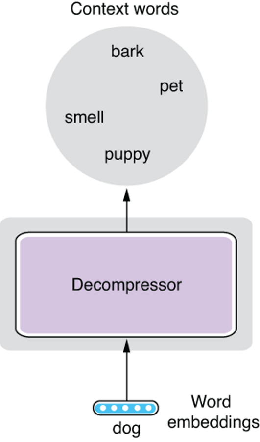
Figure 3.4 Decompressing a word vector

One way to represent a set of words mathematically is to assign a score to each word in the vocabulary. Instead of representing context words as a set, we can think of them as an associative array (dict in Python) from words to their “scores” that correspond to how related each word is to “dog,” as shown next:

{"bark": 1.4,
 "chocolate": 0.1,
 ...,
 "pet": 1.2,
 ...,
 "smell": 0.6,
 ...}

The only remaining piece of the model is how to come up with those “scores.” If you sort this list by word IDs (which may be assigned alphabetically), the scores can be conveniently represented by an N-dimensional vector, where N is the size of the entire vocabulary (the number of unique context words we consider), as follows:

[1.4, 0.1, ..., 1.2, ..., 0.6, ...]

All the “decompressor” needs to do is expand the word-embedding vector (which has three dimensions) to another vector of N dimensions.

This may sound very familiar to some of you—yes, it’s exactly what linear layers (aka fully connected layers) do. I briefly talked about linear layers in section 2.4.2, but this is a perfect time to go deeper into what they really do.

3.4.3 Linear layers

Linear layers transform a vector into another vector in a linear fashion, but how exactly do they do this? Before talking about vectors, let’s simplify and start with numbers. How would you write a function (say, a method in Python) that transforms a number into another one in a linear fashion? Remember, being linear means the output always changes by a fixed amount (say, w) if you change the input by 1, no matter what the value of the input is. For example, 2.0 * x is a linear function, because the value always increases by 2.0 if you increase x by 1, no matter what value x is. You can write a general version of such a function as follows:

def linear(x):
    return w * x + b

Let’s now assume the parameters w and b are fixed and defined somewhere else. You can confirm that the output (the return value) always changes by w if you increase or decrease x by 1. b is the value of the output when x = 0. It is called a bias in machine learning.

Now, what if there are two input variables, say, x1 and x2? Can you still write a function that transforms two input variables into another number in a linear way? Yes, and there’s very little change required to do this, as shown next:

def linear2(x1, x2):
    return w1 * x1 + w2 * x2 + b

You can confirm its linearity by checking that the output changes by w1 if you change x1 by 1, and the output changes by w2 if you change x2 by 1, regardless of the value of the other variable. Bias b is still the value of the output when x1 and x2 are both 0.

For example, assume we have w1 = 2.0, w2 = -1.0, and b = 1. For an input (1, 1), the function returns 2. If you increase x1 by 1 and give (2, 1) as the input, you’ll get 4, which is w1 more than 2. If you increase x2 by 1 and give (1, 2) as the input, you’ll get 1, which is 1 less (or w2 more) than 2.

At this point, we can start thinking about generalizing this to vectors. What if there are two output variables, say, y1 and y2? Can you still write a linear function with respect to the two inputs? Yes, you can simply duplicate the linear transformation twice, with different weights and biases, as follows:

def linear3(x1, x2):
    y1 = w11 * x1 + w12 * x2 + b1
    y2 = w21 * x1 + w22 * x2 + b2
    return [y1, y2]

OK, it’s getting a little bit complicated, but you effectively wrote a function for a linear layer that transforms a two-dimensional vector into another two-dimensional vector! If you increase the input dimension (the number of input variables), this method would get horizontally long (i.e., more additions per line), whereas if you increase the output dimension, this method would get vertically long (i.e., more lines).

In practice, deep learning libraries and frameworks implement linear layers in a more efficient, generic way, and often most of the computation happens on a GPU. However, knowing how linear layers—the most important, simplest form of neural networks—work conceptually should be essential for understanding more complex neural network models.

NOTE In AI literature, you may encounter the concept of perceptrons. A perceptron is a linear layer with only one output variable, applied to a classification problem. If you stack multiple linear layers (= perceptrons), you get a multilayer perceptron, which is basically another name for a feedforward neural network with some specific structures.

Finally, you may be wondering where the constants w and b you saw in this section come from. These are exactly the “magic constants” that I talked about in section 2.4.1. You adjust these constants so that the output of the linear layer (and the neural network as a whole) gets closer to what you want through a process called optimization. These magic constants are also called parameters of a machine learning model.

Putting this all together, the structure we want for the Skip-gram model is shown in figure 3.5. This network is very simple. It takes a word embedding as an input and expands it via a linear layer to a set of scores, one for each context word. Hopefully this is not as intimidating as many people think!

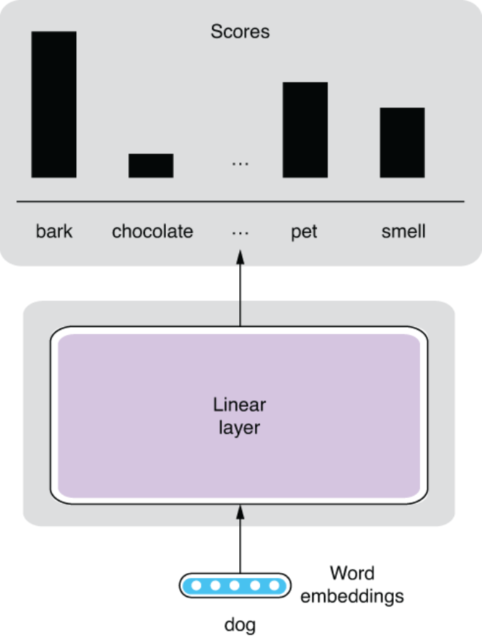
Figure 3.5 Skip-gram model structure

3.4.4 Softmax

Now let’s talk about how to “train” the Skip-gram model and learn the word embeddings we want. The key here is to turn this into a classification task, where the model predicts what words appear in the context. The “context” here simply means a window of a fixed size (e.g., 5 + 5 words on both sides) centered around the target word (e.g., “dog”). See figure 3.6 for an illustration when the window size is 2. This is actually a “fake” task because we are not interested in the prediction of the model per se, but rather in the by-product (word embeddings) produced while training the model. In machine learning and NLP, we often make up a fake task to train something else as a by-product.

Figure 3.6 Target word and context words (when window size = 2)

NOTE This setting of machine learning, where the training labels are automatically created from a given dataset, can also be called self-supervised learning. Recent popular techniques, such as word embeddings and language modeling, all use self-supervision.

It is relatively easy to make a neural network solve a classification task. You need to do the following two things:

• Modify the network so that it produces a probability distribution.

• Use cross entropy as the loss function (we’ll cover this in detail shortly).

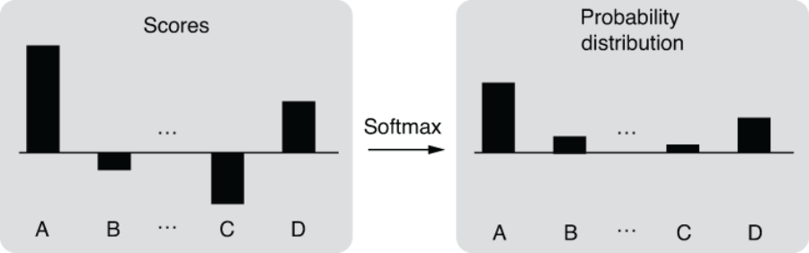
You can use something called softmax to do the first. Softmax is a function that turns a vector of K float numbers to a probability distribution, by first “squashing” the numbers so that they fit a range between 0.0-1.0, and then normalizing them so that the sum equals 1. If you are not familiar with the concept of probabilities, replace them with confidence. A probability distribution is a set of confidence values that the network places on individual predictions (in this case, context words). Softmax does all this while preserving the relative ordering of the input float numbers, so large input numbers still have large probability values in the output distribution. Figure 3.7 illustrates this conceptually.

Figure 3.7 Softmax

Another component required to turn a neural network into a classifier is cross entropy. Cross entropy is a loss function used to measure the distance between two probability distributions. It returns zero if two distributions match exactly and higher values if the two diverge. For classification tasks, we use cross entropy to compare the following:

• Predicted probability distribution produced by the neural network (output of softmax)

• Target probability distribution, where the probability of the correct class is 1.0 and everything else is 0.0

The predictions made by the Skip-gram model get closer and closer to the actual context words, and word embeddings are learned at the same time.

3.4.5 Implementing Skip-gram on AllenNLP

It is relatively straightforward to turn this model into working code using AllenNLP. Note that all the code listed in this section can be executed on the Google Colab notebook (http://realworldnlpbook.com/ch3.html#word2vec-nb). First, you need to implement a dataset reader that reads a plain text corpus and turns it into a set of instances that can be consumed by the Skip-gram model. The details of the dataset reader are not critical to the discussion here, so I’m going to omit the full code listing. You can clone the code repository of this book (https://github.com/mhagiwara/realworldnlp) and import it as follows:

from examples.embeddings.word2vec import SkipGramReader

Alternatively, if you are interested, you can see the full code from http://realworldnlpbook.com/ch3.html#word2vec. You can use the reader as follows:

reader = SkipGramReader()
text8 = reader.read('https:/./realworldnlpbook.s3.amazonaws.com/data/text8/text8')

Also, be sure to import all the necessary modules and define some constants in this example, as shown next:

from collections import Counter
 
import torch
import torch.optim as optim
from allennlp.data.data_loaders import SimpleDataLoader
from allennlp.data.vocabulary import Vocabulary
from allennlp.models import Model
from allennlp.modules.token_embedders import Embedding
from allennlp.training.trainer import GradientDescentTrainer
from torch.nn import CosineSimilarity
from torch.nn import functional
 
EMBEDDING_DIM = 256
BATCH_SIZE = 256

We are going to use the text8 (http://mattmahoney.net/dc/textdata) dataset in this example. The dataset is an excerpt from Wikipedia and is often used for training toy word embedding and language models. You can iterate over the instances in the dataset. token_in is the input token to the model, and token_out is the output (the context word):

>>> for inst in text8:
>>>     print(inst)
...
Instance with fields:
     token_in: LabelField with label: ideas in namespace: 'token_in'.'
     token_out: LabelField with label: us in namespace: 'token_out'.'
 
Instance with fields:
     token_in: LabelField with label: ideas in namespace: 'token_in'.'
     token_out: LabelField with label: published in namespace: 'token_out'.'
 
Instance with fields:
     token_in: LabelField with label: ideas in namespace: 'token_in'.'
     token_out: LabelField with label: journal in namespace: 'token_out'.'
 
Instance with fields:
     token_in: LabelField with label: in in namespace: 'token_in'.'
     token_out: LabelField with label: nature in namespace: 'token_out'.'
 
Instance with fields:
     token_in: LabelField with label: in in namespace: 'token_in'.'
     token_out: LabelField with label: he in namespace: 'token_out'.'
 
Instance with fields:
     token_in: LabelField with label: in in namespace: 'token_in'.'
     token_out: LabelField with label: announced in namespace: 'token_out'.'
...

Then, you can build the vocabulary, as we did in chapter 2, as shown next:

vocab = Vocabulary.from_instances(
    text8, min_count={'token_in': 5, 'token_out': 5})

Note that we are using min_count, which sets the lower bound on the number of occurrences for each token. Also, let’s define the data loader we use for training as follows:

data_loader = SimpleDataLoader(text8, batch_size=BATCH_SIZE)
data_loader.index_with(vocab)

Let’s then define an Embedding object that holds all the word embeddings we’d like to learn:

embedding_in = Embedding(num_embeddings=vocab.get_vocab_size('token_in'),
                         embedding_dim=EMBEDDING_DIM)

Here, EMBEDDING_DIM is the length of each word vector (number of float numbers). A typical NLP application uses word vectors of a couple hundred dimensions long (in this example, 256), but this value depends greatly on the task and the datasets. It is often suggested that you use longer word vectors as your training data grows.

Finally, you need to implement the body of the Skip-gram model, as shown next.

Listing 3.1 Skip-gram model implemented in AllenNLP

class SkipGramModel(Model):                                   ❶
 
    def __init__(self, vocab, embedding_in):
        super().__init__(vocab)
 
        self.embedding_in = embedding_in                      ❷
 
        self.linear = torch.nn.Linear(
            in_features=EMBEDDING_DIM,
            out_features=vocab.get_vocab_size('token_out'),
            bias=False)                                       ❸
 
    def forward(self, token_in, token_out):                   ❹
        
        embedded_in = self.embedding_in(token_in)             ❺
        
        logits = self.linear(embedded_in)                     ❻
 
        loss = functional.cross_entropy(logits, token_out)    ❼
 
        return {'loss': loss}

❶ AllenNLP requires every model to be inherited from Model.

❷ The embedding object is passed from outside rather than defined inside.

❸ This creates a linear layer (note that we don’t need biases).

❹ The body of neural network computation is implemented in forward().

❺ Converts input tensors (word IDs) to word embeddings

❻ Applies the linear layer

❼ Computes the loss

A few things to note:

• AllenNLP requires every model to be inherited from Model, which can be imported from allennlp.models.

• Model’s initializer (__init__) takes a Vocabulary instance and any other parameters or submodels defined externally. It also defines any internal parameters or models.

• The main computation of the model is defined in forward(). It takes all the fields from instances (in this example, token_in and token_out) as tensors (multidimensional arrays) and returns a dict that contains the 'loss' key, which will be used by the optimizer to train the model.

You can train this model using the following code.

Listing 3.2 Code for training the Skip-gram model

reader = SkipGramReader()
text8 = reader.read(' https:/./realworldnlpbook.s3.amazonaws.com/data/text8/text8')
 
vocab = Vocabulary.from_instances(
    text8, min_count={'token_in': 5, 'token_out': 5})
 
data_loader = SimpleDataLoader(text8, batch_size=BATCH_SIZE)
data_loader.index_with(vocab)
 
embedding_in = Embedding(num_embeddings=vocab.get_vocab_size('token_in'),
                         embedding_dim=EMBEDDING_DIM)
 
model = SkipGramModel(vocab=vocab,
                      embedding_in=embedding_in)
optimizer = optim.Adam(model.parameters())
 
trainer = GradientDescentTrainer(
    model=model,
    optimizer=optimizer,
    data_loader=data_loader,
    num_epochs=5,
    cuda_device=CUDA_DEVICE)
trainer.train()

Training takes a while, so I recommend truncating the training data first, say, by using only the first one million tokens. You can do this by inserting text8 = list(text8) [:1000000] after reader.read(). After the training is finished, you can get related words (words with the same meanings) using the method shown in listing 3.3. This method first obtains the word vector for a given word (token), then computes how similar it is to every other word vector in the vocabulary. The similarity is calculated using something called the cosine similarity. In simple terms, the cosine similarity is the opposite of the angle between two vectors. If two vectors are identical, the angle between them is zero, and the similarity will be 1, which is the largest possible value. If two vectors are perpendicular, the angle is 90 degrees, and the cosine will be 0. If the vectors are in totally opposite directions, the cosine will be -1.

Listing 3.3 Method to obtain related words using word embeddings

def get_related(token: str, embedding: Model, vocab: Vocabulary, 
                num_synonyms: int = 10):
    token_id = vocab.get_token_index(token, 'token_in')
    token_vec = embedding.weight[token_id]
    cosine = CosineSimilarity(dim=0)
    sims = Counter()
 
    for index, token in vocab.get_index_to_token_vocabulary('token_in').items():
        sim = cosine(token_vec, embedding.weight[index]).item()
        sims[token] = sim
 
    return sims.most_common(num_synonyms)

If you run this for words “one” and “december,” you get the lists of related words shown in table 3.1. Although you can see some words that are not related to the query word, overall, the results look good.

Table 3.1 Related words for “one” and “december"

One final note: you need to implement a couple of techniques if you want to use Skip-gram to train high-quality word vectors in practice, namely, negative sampling and subsampling of high-frequency words. Although they are important concepts, they can be a distraction if you are just starting out and would like to learn the basics of NLP. If you are interested in learning more, check out this blog post that I wrote on this topic: http://realworldnlpbook.com/ch3.html#word2vec-blog.

3.4.6 Continuous bag of words (CBOW) model

Another word-embedding model that is often mentioned along with the Skip-gram model is the continuous bag of words (CBOW) model. As a close sibling of the Skip- gram model, proposed at the same time (http://realworldnlpbook.com/ch3.html# mikolov13), the architecture of the CBOW model looks similar to that of the Skip-gram model but flipped upside down. The “fake” task the model is trying to solve is to predict the target word from a set of its context words. This is also similar to fill-in-the-blank type of questions. For example, if you see a sentence “I heard a ___ barking in the distance,” most of you can probably guess the answer “dog” instantly. Figure 3.8 shows the structure of this model.

Figure 3.8 Continuous bag of words (CBOW) model

I’m not going to implement the CBOW model from scratch here for a couple of reasons. It should be straightforward to implement if you understand the Skip-gram model. Also, the accuracy of the CBOW model measured on word semantic tasks is usually slightly lower than that of Skip-gram, and CBOW is less often used in NLP than Skip-gram. Both models are implemented in the original Word2vec (https://code .google.com/archive/p/word2vec/) toolkit, if you want to try them yourself, although the vanilla Skip-gram and CBOW models are less and less often used nowadays because of the advent of more recent, powerful word-embedding models (such as GloVe and fastText) that are covered in the rest of this chapter.

3.5 GloVe

In the previous section, I implemented Skip-gram and showed how you can train your word embeddings using large text data. But what if you wanted to build your own NLP applications leveraging high-quality word embeddings while skipping all the hassle? What if you couldn’t afford the computation and data required to train word embeddings?

Instead of training word embeddings, you can always download pretrained word embeddings published by somebody else, which many NLP practitioners do. In this section, I’m going to introduce another popular word-embedding model—GloVe, named after Global Vectors. Pretrained word embeddings generated by GloVe are probably the most widely used embeddings in NLP applications today.

3.5.1 How GloVe learns word embeddings

The main difference between the two models described earlier and GloVe is that the former is local. To recap, Skip-gram uses a prediction task where a context word (“bark”) is predicted from the target word (“dog”). CBOW basically does the opposite of this. This process is repeated as many times as there are word tokens in the dataset. It basically scans the entire dataset and asks the question, “Can this word be predicted from this other word?” for every single occurrence of words in the dataset.

Let’s think how efficient this algorithm is. What if there were two or more identical sentences in the dataset? Or very similar sentences? In that case, Skip-gram would repeat the exact same set of updates multiple times. “Can ‘bark’ be predicted from ‘dog’?” you might ask. But chances are you already asked that exact same question a couple of hundred sentences ago. If you know that the words “dog” and “bark” appear together in the context N times in the entire dataset, why repeat this N times? It’s as if you were adding “1” N times to something else (x + 1 + 1 + 1 + ... + 1) when you could simply add N to it (x + N). Could we somehow use this global information directly?

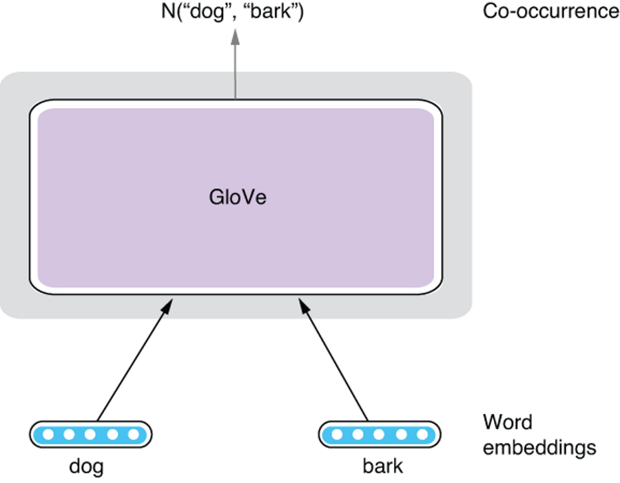
The design of GloVe is motivated by this insight. Instead of using local word co-occurrences, it uses aggregated word co-occurrence statistics in the entire dataset. Let’s say “dog” and “bark” co-occur N times in the dataset. I’m not going into the details of the model, but roughly speaking, the GloVe model tries to predict this number N from the embeddings of both words. Figure 3.9 illustrates this prediction task. It still makes some predictions about word relations, but notice that it makes one prediction per a combination of word types, but Skip-gram does so for every combination of word tokens!

Figure 3.9 GloVe

Token and Type As mentioned in section 3.3.1, a token is an occurrence of a word in text. There may be multiple occurrences of the same word in a corpus. A type, on the other hand, is a distinctive, unique word. For example, in the sentence “A rose is a rose is a rose,” there are eight tokens but only three types (“a,” “rose,” and “is”). If you are familiar with object-oriented programming, they are roughly equivalent to instance and class. There can be multiple instances of a class, but there is only one class for a concept.

3.5.2 Using pretrained GloVe vectors

In fact, not many NLP practitioners train GloVe vectors from scratch by themselves. More often, we download and use word embeddings, which are pretrained using large text corpora. This is not only quick but usually beneficial in making your NLP applications more accurate, because those pretrained word embeddings (often made public by the inventor of word-embedding algorithms) are usually trained using larger datasets and more computational power than most of us can afford. By using pretrained word embeddings, you can “stand on the shoulders of giants” and quickly leverage high-quality linguistic knowledge distilled from large text corpora.

In the rest of this section, let’s see how we can download and search for similar words using pretrained GloVe embeddings. First, you need to download the data file. The official GloVe website (https://nlp.stanford.edu/projects/glove/) provides multiple word-embedding files trained using different datasets and vector sizes. You can pick any one you like (although the file size could be large, depending on which one you choose) and unzip it. In what follows, we assume you save it under the relative path data/glove/.

Most word-embedding files are formatted in a similar way. Each line contains a word, followed by a sequence of numbers that correspond to its word vector. There are as many numbers as there are dimensions (in the GloVe files distributed on the website above, you can tell the dimensionality from the filename suffix in the form of xxxd). Each field is delimited by a space. Here is an excerpt from one of the GloVe word-embedding files:

...
if 0.15778 0.17928 -0.45811 -0.12817 0.367 0.18817 -4.5745 0.73647 ...
one 0.38661 0.33503 -0.25923 -0.19389 -0.037111 0.21012 -4.0948 0.68349 ...
has 0.08088 0.32472 0.12472 0.18509 0.49814 -0.27633 -3.6442 1.0011 ...
...

As we did in section 3.4.5, what we’d like to do is to take a query word (say, “dog”) and find its neighbors in the N-dimensional space. One way to do this is to calculate the similarity between the query word and every other word in the vocabulary and sort the words by their similarities, as shown in listing 3.3. Depending on the size of the vocabulary, this approach could be very slow. It’s like linearly scanning an array to find an element instead of using binary search.

Instead, we’ll use approximate nearest neighbor algorithms to quickly search for similar words. In a nutshell, these algorithms enable us to quickly retrieve nearest neighbors without computing the similarity between every word pair. In particular, we’ll use Annoy (https://github.com/spotify/annoy), a library for approximate neighbor search released from Spotify. You can install it by running pip install annoy. It implements a popular approximate nearest neighbor algorithm called locally sensitive hashing (LSH) using random projection.

To use Annoy to search similar words, you first need to build an index, which can be done as shown in listing 3.4. Note that we are also building a dict from word indices to words and saving it to a separate file to facilitate the word lookup later (listing 3.5).

Listing 3.4 Building an Annoy index

from annoy import AnnoyIndex
import pickle
 
EMBEDDING_DIM = 300
GLOVE_FILE_PREFIX = 'data/glove/glove.42B.300d{}'
 
def build_index():
    num_trees = 10
 
    idx = AnnoyIndex(EMBEDDING_DIM)
 
    index_to_word = {}
    with open(GLOVE_FILE_PREFIX.format('.txt')) as f:
        for i, line in enumerate(f):
            fields = line.rstrip().split(' ')
            vec = [float(x) for x in fields[1:]]
            idx.add_item(i, vec)
            index_to_word[i] = fields[0]
 
    idx.build(num_trees)
    idx.save(GLOVE_FILE_PREFIX.format('.idx'))
    pickle.dump(index_to_word,
                open(GLOVE_FILE_PREFIX.format('.i2w'), mode='wb'))

Reading a GloVe embedding file and building an Annoy index can be quite slow, but once it’s built, accessing it and retrieving similar words can be performed very quickly. This configuration is similar to search engines, where an index is built to achieve near real-time retrieval of documents. This is suitable for applications where retrieval of similar items in real time is required but update of the dataset happens less frequently. Examples include search engines and recommendation engines.

Listing 3.5 Using an Annoy index to retrieve similar words

def search(query, top_n=10):
    idx = AnnoyIndex(EMBEDDING_DIM)
    idx.load(GLOVE_FILE_PREFIX.format('.idx'))
    index_to_word = pickle.load(open(GLOVE_FILE_PREFIX.format('.i2w'),
                                     mode='rb'))
    word_to_index = {word: index for index, word in index_to_word.items()}
    
    query_id = word_to_index[query]
    word_ids = idx.get_nns_by_item(query_id, top_n)
    for word_id in word_ids:
        print(index_to_word[word_id])

If you run this for the words “dog” and “december,” you’ll get the lists of the 10 most-related words shown in table 3.2.

Table 3.2 Related words for “dog” and “december"

You can see that each list contains many related words to the query word. You see the identical words at the top of each list—this is because the cosine similarity of two identical vectors is always 1, its maximum possible value.

3.6 fastText

In the previous section, we saw how to download pretrained word embeddings and retrieve related words. In this section, I’ll explain how to train word embeddings using your own text data using fastText, a popular word-embedding toolkit. This is handy when your textual data is not in a general domain (e.g., medical, financial, legal, and so on) and/or is not in English.

3.6.1 Making use of subword information

All the word-embedding methods we’ve seen so far in this chapter assign a distinct word vector for each word. For example, word vectors for “dog” and “cat” are treated distinctly and are independently trained at the training time. At first glance, there seems to be nothing wrong about this. After all, they are separate words. But what if the words were, say, “dog” and “doggy?” Because “-y” is an English suffix that denotes some familiarity and affection (other examples include “grandma” and “granny” and “kitten” and “kitty”), these pairs of words have some semantic connection. However, word-embedding algorithms that treat words as distinct cannot make this connection. In the eyes of these algorithms, “dog” and “doggy” are nothing more than, say, word_823 and word_1719.

This is obviously limiting. In most languages, there’s a strong connection between word orthography (how you write words) and word semantics (what they mean). For example, words that share the same stems (e.g., “study” and “studied,” “repeat” and “repeatedly,” and “legal” and “illegal”) are often related. By treating them as separate words, word-embedding algorithms are losing a lot of information. How can they leverage word structures and reflect the similarities in the learned word embeddings?

fastText, an algorithm and a word-embedding library developed by Facebook, is one such model. It uses subword information, which means information about linguistic units that are smaller than words, to train higher-quality word embeddings. Specifically, fastText breaks words down to character n-grams (section 3.2.3) and learns embeddings for them. For example, if the target word is “doggy,” it first adds special symbols at the beginning and end of the word and learns embeddings for <do, dog, ogg, ggy, gy>, when n = 3. The vector for “doggy” is simply the sum of all these vectors. The rest of the architecture is quite similar to that of Skip-gram. Figure 3.10 shows the structure of the fastText model.

Figure 3.10 Architecture of fastText

Another benefit in leveraging subword information is that it can alleviate the out-of-vocabulary (OOV) problem. Many NLP applications and models assume a fixed vocabulary. For example, a typical word-embedding algorithm such as Skip-gram learns word vectors only for the words that were encountered in the train set. However, if a test set contains words that did not appear in the train set (which are called OOV words), the model would be unable to assign any vectors to them. For example, if you train Skip-gram word embeddings from books published in the 1980s and apply them to modern social media text, how would it know what vectors to assign to “Instagram”? It won’t. On the other hand, because fastText uses subword information (character n-grams), it can assign word vectors to any OOV words, as long as they contain character n-grams seen in the training data (which is almost always the case). It can potentially guess it’s related to something quick (“Insta”) and pictures (“gram”).

3.6.2 Using the fastText toolkit

Facebook provides the open source for the fastText toolkit, a library for training the word-embedding model discussed in the previous section. In the remainder of this section, let’s see how it feels like to use this library to train word embeddings.

First, go to their official documentation (http://realworldnlpbook.com/ch3.html #fasttext) and follow the instruction to download and compile the library. It is just a matter of cloning the GitHub repository and running make from the command line in most environments. After compilation is finished, you can run the following command to train a Skip-gram-based fastText model:

$ ./fasttext skipgram -input ../data/text8 -output model

We are assuming there’s a text data file under ../data/text8 that you’d like to use as the training data, but change this if necessary. This will create a model.bin file, which is a binary representation of the trained model. After training the model, you can obtain word vectors for any words, even for the ones that you’ve never seen in the training data, as follows:

$ echo "supercalifragilisticexpialidocious" 
| ./fasttext print-word-vectors model.bin
supercalifragilisticexpialidocious 0.032049 0.20626 -0.21628 -0.040391 -0.038995 0.088793 -0.0023854 0.41535 -0.17251 0.13115 ...

3.7 Document-level embeddings

All the models I have described so far learn embeddings for individual words. If you are concerned only with word-level tasks such as inferring word relationships, or if they are combined with more powerful neural network models such as recurrent neural networks (RNNs), they can be very useful tools. However, if you wish to solve NLP tasks that are concerned with larger linguistic structures such as sentences and documents using word embeddings and traditional machine learning tools such as logistic regression and support vector machines (SVMs), word-level embedding methods are still limited. How can you represent larger linguistic units such as sentences using vector representations? How can you use word embeddings for sentiment analysis, for example?

One way to achieve this is to simply use the average of all word vectors in a sentence. You can average vectors by taking the average of first elements, second elements, and so on and make a new vector by combining these averaged numbers. You can use this new vector as an input to traditional machine learning models. Although this method is simple and can be effective, it is also very limiting. The biggest issue is that it cannot take word order into consideration. For example, both sentences “Mary loves John.” and “John loves Mary.” would have exactly the same vectors if you simply averaged word vectors for each word in the sentence.

NLP researchers have proposed models and algorithms that can specifically address this issue. One of the most popular is Doc2Vec, originally proposed by Le and Mikolov in 2014 (https://cs.stanford.edu/~quocle/paragraph_vector.pdf). This model, as its name suggests, learns vector representations for documents. In fact, “document” here simply means any variable-length piece of text that contains multiple words. Similar models are also called under many similar names such as Sentence2Vec, Paragraph2Vec, paragraph vectors (this is what the authors of the original paper used), but in essence, they all refer to the variations of the same model.

In the rest of this section, I’m going to discuss one of the Doc2Vec models called distributed memory model of paragraph vectors (PV-DM). The model looks very similar to CBOW, which we studied earlier in this chapter, but with one key difference—one additional vector, called paragraph vector, is added as an input. The model predicts the target word from a set of context words and the paragraph vector. Each paragraph is assigned a distinct paragraph vector. Figure 3.11 shows the structure of this PV-DM model. Also, PV-DM uses only context words that come before the target word for prediction, but this is a minor difference.

Figure 3.11 Distributed memory model of paragraph vectors

What effect would this paragraph vector have on the prediction task? Now you have some extra information from the paragraph vector for predicting the target word. As the model tries to maximize the prediction accuracy, you can expect that the paragraph vector is updated so that it provides some useful “context” information in the sentence that is not collectively captured by the context word vectors. As a by-product, the model learns something that reflects the overall meaning of each paragraph, along with word vectors.

Several open source libraries and packages support Doc2Vec models, but one of the most widely used is Gensim (https://radimrehurek.com/gensim/), which can be installed by running pip install gensim. Gensim is a popular NLP toolkit that supports a wide range of vector and topic models such as TF-IDF (term frequency and inverse document frequency), LDA (latent semantic analysis), and word embeddings.

To train a Doc2Vec model using Gensim, you first need to read a dataset and convert documents to TaggedDocument. This can be done using the read_corpus() method shown here:

from gensim.utils import simple_preprocess
from gensim.models.doc2vec import TaggedDocument
 
def read_corpus(file_path):
    with open(file_path) as f:
        for i, line in enumerate(f):
            yield TaggedDocument(simple_preprocess(line), [i])

We are going to use a small dataset consisting of the first 200,000 English sentences taken from the Tatoeba project (https://tatoeba.org/). You can download the dataset from http://mng.bz/7l0y. Then you can use Gensim’s Doc2Vec class to train the Doc2Vec model and retrieve similar documents based on the trained paragraph vectors, as demonstrated next.

Listing 3.6 Training a Doc2Vec model and retrieving similar documents

    from gensim.models.doc2vec import Doc2Vec
    
    train_set = list(read_corpus('data/mt/sentences.eng.200k.txt'))
    model = Doc2Vec(vector_size=256, min_count=3, epochs=30)
    model.build_vocab(train_set)
    model.train(train_set,
                total_examples=model.corpus_count,
                epochs=model.epochs)
 
    query_vec = model.infer_vector(
        ['i', 'heard', 'a', 'dog', 'barking', 'in', 'the', 'distance'])
    sims = model.docvecs.most_similar([query_vec], topn=10)
    for doc_id, sim in sims:
        print('{:3.2f} {}'.format(sim, train_set[doc_id].words)) 

This will show you a list of documents similar to the input document “I heard a dog barking in the distance,” as follows:

0.67 ['she', 'was', 'heard', 'playing', 'the', 'violin']
0.65 ['heard', 'the', 'front', 'door', 'slam']
0.61 ['we', 'heard', 'tigers', 'roaring', 'in', 'the', 'distance']
0.61 ['heard', 'dog', 'barking', 'in', 'the', 'distance']
0.60 ['heard', 'the', 'door', 'open']
0.60 ['tom', 'heard', 'the', 'door', 'open']
0.60 ['she', 'heard', 'dog', 'barking', 'in', 'the', 'distance']
0.59 ['heard', 'the', 'door', 'close']
0.59 ['when', 'he', 'heard', 'the', 'whistle', 'he', 'crossed', 'the', 'street']
0.58 ['heard', 'the', 'telephone', 'ringing']

Notice that most of the retrieved sentences here are related to hearing sound. In fact, an identical sentence is in the list, because I took the query sentence from Tatoeba in the first place! Gensim’s Doc2Vec class has a number of hyperparameters that you can use to tweak the model. You can read further about the class on their reference page (https://radimrehurek.com/gensim/models/doc2vec.html).

3.8 Visualizing embeddings

In the final section of this chapter, we are going to shift our focus on visualizing word embeddings. As we’ve done earlier, retrieving similar words given a query word is a great way to quickly check if word embeddings are trained correctly. But it gets tiring and time-consuming if you need to check a number of words to see if the word embeddings are capturing semantic relationships between words as a whole.

As mentioned earlier, word embeddings are simply N-dimensional vectors, which are also “points” in an N-dimensional space. We were able to see those points visually in a 3-D space in figure 3.1 because N was 3. But N is typically a couple of hundred in most word embeddings, and we cannot simply plot them on an N-dimensional space.

A solution is to reduce the dimension down to something that we can see (two or three dimensions) while preserving relative distances between points. This technique is called dimensionality reduction. We have a number of ways to reduce dimensionality, including PCA (principal component analysis) and ICA (independent component analysis), but by far the most widely used visualization technique for word embeddings is called t-SNE (t-distributed Stochastic Neighbor Embedding, pronounced “tee-snee). Although the details of t-SNE are outside the scope of this book, the algorithm tries to map points to a lower-dimensional space by preserving the relative neighboring relationship between points in the original high-dimensional space.

The easiest way to use t-SNE is to use Scikit-Learn (https://scikit-learn.org/), a popular Python library for machine learning. After installing it (usually just a matter of running pip install scikit-learn), you can use it to visualize the GloVe vectors read from a file as shown next (we use Matplotlib to draw the plot).

Listing 3.7 Using t-SNE to visualize GloVe embeddings

from sklearn.manifold import TSNE
import matplotlib.pyplot as plt
 
def read_glove(file_path):
    with open(file_path) as f:
        for i, line in enumerate(f):
            fields = line.rstrip().split(' ')
            vec = [float(x) for x in fields[1:]]
            word = fields[0]
            yield (word, vec)
 
words = []
vectors = []
for word, vec in read_glove('data/glove/glove.42B.300d.txt'):
    words.append(word)
    vectors.append(vec)
 
model = TSNE(n_components=2, init='pca', random_state=0)
coordinates = model.fit_transform(vectors)
 
plt.figure(figsize=(8, 8))
 
for word, xy in zip(words, coordinates):
    plt.scatter(xy[0], xy[1])
    plt.annotate(word,
                 xy=(xy[0], xy[1]),
                 xytext=(2, 2),
                 textcoords='offset points')
 
plt.xlim(25, 55)
plt.ylim(-15, 15)
plt.show()

In listing 3.7, I used xlim() and ylim() to limit the plotted range to magnify some areas that are of interest to us. You may want to try different values to focus on other areas in the plot.

The code in listing 3.7 generates the plot shown in figure 3.12. There’s a lot of interesting stuff going on here, but at a quick glance, you will notice the following clusters of words that are semantically related:

• Bottom-left: web-related words (posts, article, blog, comments, . . . ).

• Upper-left: time-related words (day, week, month, year, . . . ).

• Middle: numbers (0, 1, 2, . . . ). Surprisingly, these numbers are lined up in an increasing order toward the bottom. GloVe figured out which numbers are larger purely from a large amount of textual data.

• Bottom-right: months (january, february, . . . ) and years (2004, 2005, . . . ). Again, the years seem to be lined up in an increasing order, almost in parallel with the numbers (0, 1, 2, . . . ).

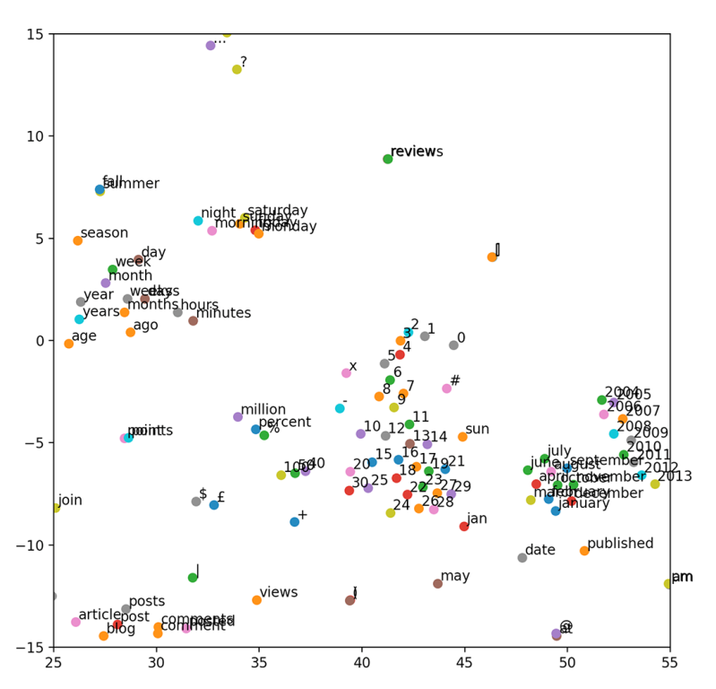
Figure 3.12 GloVe embeddings visualized by t-SNE

If you think about it, it’s an incredible feat for a purely mathematical model to figure out these relationships among words, all from a large amount of text data. Hopefully, now you know how much of an advantage it is if the model knows “july” and “june” are closely related compared to needing to figure everything out starting from word_823 and word_1719.

Summary

• Word embeddings are numeric representations of words, and they help convert discrete units (words and sentences) to continuous mathematical objects (vectors).

• The Skip-gram model uses a neural network with a linear layer and softmax to learn word embeddings as a by-product of the “fake” word-association task.

• GloVe makes use of global statistics of word co-occurrence to train word embeddings efficiently.

• Doc2Vec and fastText learn document-level embeddings and word embeddings with subword information, respectively.

• You can use t-SNE to visualize word embeddings.