6 Sequence-to-sequence models

This chapter covers

• Building a machine translation system using Fairseq
• Transforming one sentence to another using a Seq2Seq model
• Using a beam search decoder to generate better output
• Evaluating the quality of machine translation systems
• Building a dialogue system (chatbot) using a Seq2Seq model

In this chapter, we are going to discuss sequence-to-sequence (Seq2Seq) models, which are some of the most important complex NLP models and are used for a wide range of applications, including machine translation. Seq2Seq models and their variations are already used as the fundamental building blocks in many real-world applications, including Google Translate and speech recognition. We are going to build a simple neural machine translation system using a powerful framework to learn how the models work and how to generate the output using greedy and beam search algorithms. At the end of this chapter, we will build a chatbot—an NLP application with which you can have a conversation. We’ll also discuss the challenges and limitations of simple Seq2Seq models.

6.1 Introducing sequence-to-sequence models

In the previous chapter, we discussed two types of powerful NLP models, namely, sequential labeling and language models. To recap, a sequence-labeling model takes a sequence of some units (e.g., words) and assigns a label (e.g., a part-of-speech (POS) tag) to each unit, whereas a language model takes a sequence of some units (e.g., words) and estimates how probable the given sequence is in the domain in which the model is trained. You can also use a language model to generate realistic-looking text from scratch. See figure 6.1 for the overview of these two models.

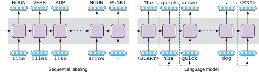
Figure 6.1 Sequential labeling and language models

Although these two models are useful for a number of NLP tasks, for some, you may want the best of both worlds—you may want your model to take some input (e.g., a sentence) and generate something else (e.g., another sentence) in response. For example, if you wish to translate some text written in one language into another, you need your model to take a sentence and produce another. Can you do this with sequential-labeling models? No, because they can produce only the same number of output labels as there are tokens in the input sentence. This is obviously too limiting for translation—one expression in a language (say, “Enchanté” in French) can have an arbitrarily large or small number of words in another (say, “Nice to meet you” in English). Can you do this with language models? Again, not really. Although you can generate realistic-looking text using language models, you have almost no control over the text they generate. In fact, language models do not take any input.

But if you look at figure 6.1 more carefully, you might notice something. The model on the left (the sequential-labeling model) takes a sentence as its input and produces some form of representations, whereas the model on the right produces a sentence with variable length that looks like natural language text. We already have the components needed to build what we want, that is, a model that takes a sentence and transforms it into another. The only missing part is a way to connect these two so that we can control what the language model generates.

In fact, by the time the model on the left finishes processing the input sentence, the RNN has already produced its abstract representation, which is encoded in the RNN’s hidden states. If you can simply connect these two so that the sentence representation is passed from left to right and the language model can generate another sentence based on the representation, it seems like you can achieve what you wanted to do in the first place!

Sequence-to-sequence models—or Seq2Seq models, in short—are built on this insight. A Seq2Seq model consists of two subcomponents—an encoder and a decoder. See figure 6.2 for an illustration. An encoder takes a sequence of some units (e.g., a sentence) and converts it into some internal representation. A decoder, on the other hand, generates a sequence of some units (e.g., a sentence) from the internal representation. As a whole, a Seq2Seq model takes a sequence and generates another sequence. As with the language model, the generation stops when the decoder produces a special token, <END>, which enables a Seq2Seq model to generate an output that can be longer or shorter than the input sequence.

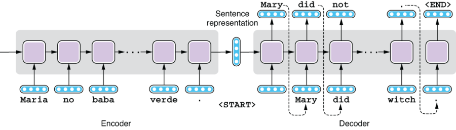
Figure 6.2 Sequence-to-sequence model

Many variants of Seq2Seq models exist, depending on what architecture you use for the encoder, what architecture you use for the decoder, and how information flows between the two. This chapter covers the most basic type of Seq2Seq model—simply connecting two RNNs via the sentence representation. We’ll discuss more advanced variants in chapter 8.

Machine translation is the first, and by far the most popular, application of Seq2Seq models. However, the Seq2Seq architecture is a generic model applicable to numerous NLP tasks. In one such task, summarization, an NLP system takes a long text (e.g., a news article) and produces its summary (e.g., a news headline). A Seq2Seq model can be used to “translate” the longer text into the shorter one. Another task is a dialogue system, or a chatbot. If you think of a user’s utterance as the input and the system’s response as the output, the dialogue system’s job is to “translate” the former into the latter. Later in this chapter, we will discuss a case study where we actually build a chatbot using a Seq2Seq model. Yet another (somewhat surprising) application is parsing—if you think of the input text as one language and its syntax representation as another, you can parse natural language texts with a Seq2Seq model.¹

6.2 Machine translation 101

We briefly touched upon machine translation in section 1.2.1. To recap, machine translation (MT) systems are NLP systems that translate a given text from one language to another. The language the input text is written in is called the source language, whereas the one for the output is called the target language. The combination of the source and target languages is called the language pair.

First, let’s look at a couple of examples to see what it’s like and why it’s difficult to translate a foreign language to English (or any other language you understand). In the first example, let’s translate a Spanish sentence, “Maria no daba una bofetada a la bruja verde.” to the English counterpart, “Mary did not slap the green witch.” A common practice in illustrating the process of translation is to draw how words or phrases of the same meaning map between the two sentences. Correspondence of linguistic units between two instances is called alignment. Figure 6.3 shows the alignment between the Spanish and English sentences.

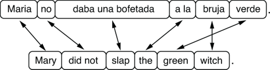
Figure 6.3 Translation and word alignment between Spanish and English

Some words (e.g., “Maria” and “Mary,” “bruja” and “witch,” and “verde” and “green”) match exactly one to one. However, some expressions (e.g., “daba una bofetada” and “slap”) differ in such a significant way that you can only align phrases between Spanish and English. Finally, even where there’s one-to-one correspondence between words, the way words are arranged, or word order, may differ between the two languages. For example, adjectives are added after nouns in Spanish (“la bruja verde”) whereas in English, they come before nouns (“the green witch”). Spanish and English are linguistically similar in terms of grammar and vocabulary, especially when compared to, say, Chinese and English, although this single example shows translating between the two may be a challenging task.

Things start to look more complicated between Mandarin Chinese and English. Figure 6.4 illustrates the alignment between a Chinese sentence (“Bushi yu Shalong juxing le huitan.”) and its English translation (“Bush held a talk with Shalon.”). Although Chinese uses ideographic characters of its own, we use romanized sentences here for simplicity.

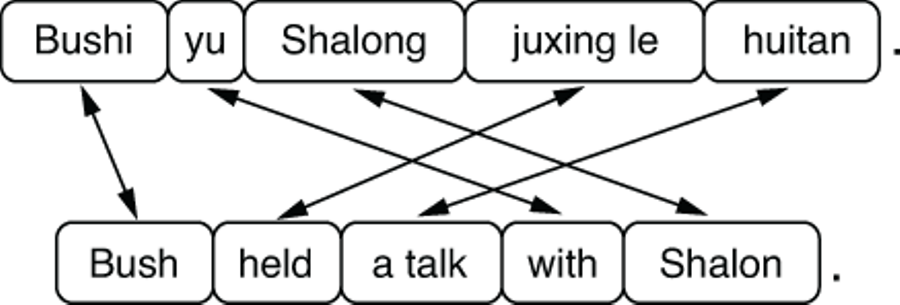
Figure 6.4 Translation and word alignment between Mandarin Chinese and English

You can now see more crossing arrows in the figure. Unlike English, Chinese prepositional phrases such as “with Shalon” are usually attached to verbs from the left. Also, the Chinese language doesn’t explicitly mark tense, and MT systems (and human translators alike) need to “guess” the correct tense to use for the English translation. Finally, Chinese-to-English MT systems also need to infer the correct number (singular or plural) of each noun, because Chinese nouns are not explicitly marked according to their number (e.g., “huitan” just means “talk” with no explicit mention of number). This is a good example showing how the difficulty of translation depends on the language pair. Development of MT systems between linguistically different languages (such as Chinese and English) is usually more challenging than those between linguistically similar ones (such as Spanish and Portuguese).

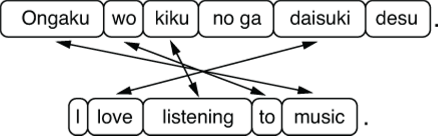
Figure 6.5 Translation and word alignment between Japanese and English

Let’s take a look at one more example—translating from Japanese to English, illustrated in figure 6.5. All the arrows in the figure are crossed, meaning that the word order is almost exactly opposite in these two sentences. In addition to the fact that Japanese prepositional phrases (“to music”) and relative clauses attach from the left like Chinese, objects (such as “listening” in “I love listening” in the example) come before the verb. In other words, Japanese is an SOV (subject-object-verb) language, whereas all the other languages we mentioned so far (English, Spanish, and Chinese) are SVO (subject-verb-object) languages. Structural differences are a reason why direct, word-to-word translation doesn’t work very well.

NOTE This word-order classification system of language (such as SOV and SVO) is often used in linguistic typology. The vast majority of world languages are either SOV (most common) or SVO (slightly less common), although a small number of languages follow other word-order systems, such as VSO (verb-subject-object), used by Arabic and Irish, for example. Very few languages (less than 3% of all languages) follow other types (VOS, OVS, and OSV).

Besides the structural differences shown in the previous figures, many other factors can make MT a difficult task. One such factor is lexical difference. If you are translating, for example, the Japanese word “ongaku” to the English “music,” there’s little ambiguity. “Ongaku” is almost always “music.” However, if you are translating, say, the English word “brother” to Chinese, you face ambiguity, because Chinese uses distinct words for “elder brother” and “younger brother.” In an even more extreme case, if you are translating “cousin” to Chinese, you have eight different choices, because in the Chinese family system, you need to use distinct words depending on whether your cousin is maternal or paternal, female or male, and older or younger than you.

Another factor that makes MT challenging is omission. You can see that in figure 6.5, there’s no Japanese word for “I.” In languages such as Chinese, Japanese, Spanish, and many others, you can omit the subject pronoun when it’s clear from the context and/or the verb form. This is called zero pronoun, and it can become a problem when translating from a pronoun-dropping language to a language where it happens less often (e.g., English).

One of the earliest MT systems, developed during the Georgetown-IBM experiment, was built to translate Russian sentences into English during the Cold War. But all it did was not much different from looking up each word in a bilingual dictionary and replacing it with its translation. The three examples shown above should be enough to convince you that simply replacing word by word is too limiting. Later systems incorporated a larger set of lexicons and grammar rules, but these rules are written manually by linguists and are not enough to capture the complexities of language (again, remember the poor software engineer from chapter 1).

The main paradigm for MT that remained dominant both in academia and industry before the advent of neural machine translation (NMT) is called statistical machine translation (SMT). The idea behind it is simple: learn how to translate from data, not by manually crafting rules. Specifically, SMT systems learn how to translate from datasets that contain a collection of texts in the source language and their translation in the target language. Such datasets are called parallel corpora (or parallel texts, or bitexts). By looking at a collection of paired sentences in both languages, the algorithm seeks patterns of how words in one language should be translated to another. The resulting statistical model is called a translation model. At the same time, by looking at a collection of target sentences, the algorithm can learn what valid sentences in the target languages should look like. Sounds familiar? This is exactly what a language model is all about (see the previous chapter). The final SMT model combines these two models and produces output that is a plausible translation of the input and is a valid, fluent sentence in the target language on its own.

Around 2015, the advent of powerful neural machine translation (NMT) models subverted the dominance of SMT. SMT and NMT have two key differences. First, by definition, NMT is based on neural networks, which are well known for their power to model language accurately. As a result, target sentences generated by NMT tend to be more fluent and natural than those generated by SMT. Second, NMT models are trained end-to-end, as I briefly touched on in chapter 1. This means that NMT models consist of a single neural network that takes an input and directly produces an output, instead of a patchwork of submodels and submodules that you need to train independently. As a result, NMT models are simpler to train and smaller in code size than SMT models.

MT is already used in many different industries and aspects of our lives. Translating foreign text into a language that you understand to grasp its meaning quickly is called gisting. If the text is deemed important enough after gisting, it may be sent to formal, manual translation. Professional translators also use MT for their work. Oftentimes, the source text is first translated to the target language using an MT system, then the produced text is edited by human translators. Such editing is called postediting. The use of automated systems (called computer-aided translation, or CAT) can accelerate the translation process and reduce the cost.

6.3 Building your first translator

In this section, we are going to build a working MT system. Instead of writing any Python code to do that, we’ll make the most of existing MT frameworks. A number of open source frameworks make it easier to build MT systems, including Moses (http://www.statmt.org/moses/) for SMT and OpenNMT (http://opennmt.net/) for NMT. In this section, we will use Fairseq (https://github.com/pytorch/fairseq), an NMT toolkit developed by Facebook that is becoming more and more popular among NLP practitioners these days. The following aspects make Fairseq a good choice for developing an NMT system quickly: 1) it is a modern framework that comes with a number of predefined state-of-the-art NMT models that you can use out of the box; 2) it is very extensible, meaning you can quickly implement your own model by following their API; and 3) it is very fast, supporting multi-GPU and distributed training by default. Thanks to its powerful models, you can build a decent quality NMT system within a couple of hours.

Before you start, install Fairseq by running pip install fairseq in the root of your project directory. Also, run the following commands in your shell to download and expand the dataset (you may need to install unzip if you are using Ubuntu by running sudo apt-get install unzip):²

$ mkdir -p data/mt
$ wget https://realworldnlpbook.s3.amazonaws.com/data/mt/tatoeba.eng_spa.zip
$ unzip tatoeba.eng_spa.zip -d data/mt

We are going to use Spanish and English parallel sentences from the Tatoeba project, which we used previously in chapter 4, to train a Spanish-to-English MT system. The corpus consists of approximately 200,000 English sentences and their Spanish translations. I went ahead and already formatted the dataset so that you can use it without worrying about obtaining the data, tokenizing the text, and so on. The dataset is already split into train, validate, and test subsets.

6.3.1 Preparing the datasets

As mentioned previously, MT systems (both SMT and NMT) are machine learning models and thus are trained from data. The development process of MT systems looks similar to any other modern NLP systems, as shown in figure 6.6. First, the training portion of the parallel corpus is preprocessed and used to train a set of NMT model candidates. Next, the validation portion is used to choose the best-performing model out of all the candidates. This process is called model selection (see chapter 2 for a review). Finally, the best model is tested on the test portion of the dataset to obtain evaluation metrics, which reflect how good the model is.

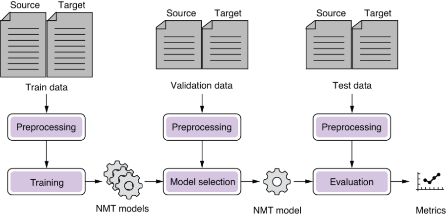
Figure 6.6 Pipeline for building an NMT system

The first step in MT development is preprocessing the dataset. But before preprocessing, you need to convert the dataset into an easy-to-use format, which is usually plain text in NLP. In practice, the raw data for training MT systems come in many different formats, for example, plain text files (if you are lucky), XML formats of proprietary software, PDF files, and database records. Your first job is to format the raw files so that source sentences and their target translations are aligned sentence by sentence. The resulting file is often a TSV file where each line is a tab-separated sentence pair, which looks like the following:

Let's try something.                   Permíteme intentarlo.
Muiriel is 20 now.                     Ahora, Muiriel tiene 20 años.
I just don't know what to say.         No sé qué decir.
You are in my way.                     Estás en mi camino.
Sometimes he can be a strange guy.     A veces él puede ser un chico raro.
...

After the translations are aligned, the parallel corpus is fed into the preprocessing pipeline. Specific operations applied in this process differ from application to application, and from language to language, but the following steps are most common:

1. Filtering

2. Cleaning

3. Tokenization

In the filtering step, any sentence pairs that are not suitable for training an MT system are removed from the dataset. What makes a sentence pair not suitable depends on many factors, but, for example, any sentence pair where either text is too long (say, more than 1,000 words) is not useful, because most MT models are not capable of modeling such a long sentence. Also, any sentence pairs where one sentence is too long but the other is too short are probably noise caused by a data processing or alignment error. For example, if a Spanish sentence is 10 words long, the length of its English translation should fall within a 5- to 15-word range. Finally, if, for any reason, the parallel corpus contains any languages other than the source and target languages, you should remove such sentence pairs. This happens a lot more often than you’d imagine—many documents are multilingual due to, for example, quotes, explanation, or code switching (mixing more than one language in a sentence). Language detection (see chapter 4) can help detect such anomalies.

After filtering, sentences in the dataset can be cleaned further. This process may include such things as removal of HTML tags and any special characters and normalization of characters (e.g., traditional and simplified Chinese) and spelling (e.g., American and British English).

If the target language uses scripts such as the Latin (a, b, c, ...) or Cyrillic (а, б, в, ...) alphabets, which distinguish upper- and lowercases, you may want to normalize case. By doing so, your MT system will group “NLP” with “nlp” and “Nlp.” This step is usually a good thing, because by having three different representations of a single concept, the MT model needs to learn that they are in fact a single concept purely from the data. Normalizing cases also reduces the number of distinct words, which makes training and prediction faster. However, this also groups “US” and “Us” and “us,” which might not be a desirable behavior, depending on the type of data and the domain you are working with. In practice, such decisions, including whether to normalize cases, are carefully made by observing their effect on the validation data performance.

At this point, the dataset is still a bunch of strings of characters. Most MT systems operate on words, so you need to tokenize the input (section 3.3) to identify words. Depending on the language, you may need to run a different pipeline (e.g., word segmentation is needed for Chinese and Japanese).

The Tatoeba dataset you downloaded and expanded earlier has already gone through all this preprocessing pipeline. Now you are ready to hand the dataset over to Fairseq. The first step is to tell Fairseq to convert the input files to the binary format so that the training script can read them easily, as follows:

$ fairseq-preprocess 
      --source-lang es 
      --target-lang en 
      --trainpref data/mt/tatoeba.eng_spa.train.tok 
      --validpref data/mt/tatoeba.eng_spa.valid.tok 
      --testpref data/mt/tatoeba.eng_spa.test.tok 
      --destdir data/mt-bin 
      --thresholdsrc 3 
      --thresholdtgt 3

When this succeeds, you should see a message Wrote preprocessed data to data/mt-bin on your terminal. You should also find the following group of files under the data/mt-bin directory:

dict.en.txt dict.es.txt  test.es-en.en.bin  test.es-en.en.idx  test.es-en.es.bin  test.es-en.es.idx  train.es-en.en.bin  train.es-en.en.idx  train.es-en.es.bin  train.es-en.es.idx  valid.es-en.en.bin  valid.es-en.en.idx  valid.es-en.es.bin  valid.es-en.es.idx

One of the key functionalities of this preprocessing step is to build the vocabulary (called the dictionary in Fairseq), which is a mapping from vocabulary items (usually words) to their IDs. Notice the two dictionary files in the directory, dict.en.txt and dict.es.txt. MT deals with two languages, so the system needs to maintain two mappings, one for each language.

6.3.2 Training the model

Now that the train data is converted into the binary format, you are ready to train the MT model. Invoke the fairseq-train command with the directory where the binary files are located, along with several hyperparameters, as shown next:

$ fairseq-train 
    data/mt-bin 
    --arch lstm 
    --share-decoder-input-output-embed 
    --optimizer adam 
    --lr 1.0e-3 
    --max-tokens 4096 
    --save-dir data/mt-ckpt

You don’t have to worry about understanding what most of the parameters here mean (just yet). At this point, you need to know only that you are training a model using the data stored in the directory specified by the first parameter (data/mt-bin) using an LSTM architecture (—arch lstm) with a bunch of other hyperparameters, and saving the results in data/mt-ckpt (short for “checkpoint”).

When you run this command, your terminal will show two types of progress bars alternatively—one for training and another for validating, as shown here:

| epoch 001:  16%|???▏                | 61/389 [00:13<01:23,  3.91it/s, loss=8.347, ppl=325.58, wps=17473, ups=4, wpb=3740.967, bsz=417.180, num_updates=61, lr=0.001, gnorm=2.099, clip=0.000, oom=0.000, wall=17, train_wall=12]
 
| epoch 001 | valid on 'valid' subset | loss 4.208 | ppl 18.48 | num_updates 389

The lines corresponding to validation results are easily distinguishable by their contents—they say “valid” subset. For each epoch, the training process alternates two stages: training and validation. An epoch, a concept used in machine learning, means one pass through the entire train data. In the training stage, the loss is calculated using the training data, then the model parameters are adjusted in such a way that the new set of parameters lowers the loss. In the validation stage, the model parameters are fixed, and a separate dataset (validation set) is used to measure how well the model is performing against the dataset.

I mentioned in chapter 1 that validation sets are used for model selection, a process where the best machine learning model is chosen among all the possible models trained from a single training set. Here, by alternating between training and validation stages, we use the validation set to check the performance of all the intermediary models (i.e., the model after the first epoch, the one after two epochs, and so on). In other words, we use the validation stage to monitor the progress of the training.

Why is this a good idea? We gain many benefits by inserting the validation stage after every epoch, but the most important one is to avoid overfitting—the very reason why a validation data is important in the first place. To illustrate this further, let’s look at how the loss changes over the course of the training of our Spanish-to-English MT model, for both the train and the validation sets, as shown in figure 6.7.

As the training continues, the train loss becomes smaller and smaller and gradually approaches zero, because this is exactly what we told the optimizer to do: decrease the loss as much as possible. Checking whether the train loss is decreasing steadily epoch after epoch is a good “sanity check” that your model and the training pipeline are working as expected.

On the other hand, if you look at the validation loss, it goes down at first for several epochs, but after a certain point, it gradually goes back up, forming a U-shaped curve—a typical sign of overfitting. After several epochs of training, your model fits the train set so well that it begins to lose its generalizability on the validation set.

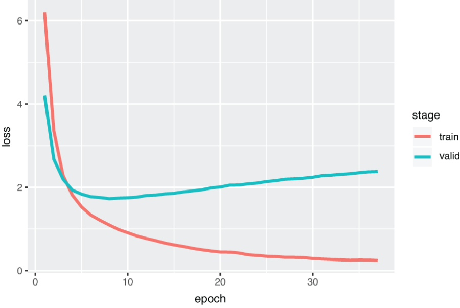
Figure 6.7 Train and validation loss

Let’s use a concrete example in MT to illustrate what’s really going on when a model is overfitted. For example, if your training data contains the English sentence “It is raining hard” and its Spanish translation “Esta lloviendo fuerte,” with no other sentences having the word “hard” in them, the overfitted model may believe that “fuerte” is the only possible translation of “hard.” A properly fitted model might leave some wiggle room for other Spanish words to appear as a translation for “hard,” but an overfitted MT system would always translate “hard” to “fuerte,” which is the “correct” thing to do according to the train set but obviously not ideal if you’d like to build a robust MT system. For example, the best way to translate “hard” in “She is trying hard” is not “fuerte.”

If you see your validation loss starting to creep up, there’s little point keeping the training process running, because chances are, your model has already overfitted to the data to some extent. A common practice in such a situation, called early stopping, is to terminate the training. Specifically, if your validation loss is not improving for a certain number of epochs, you stop the training and use the model at the point when the validation loss was the lowest. The number of epochs you wait until the training is terminated is called patience. In practice, the metric you care about the most (such as BLEU; see section 6.5.2) is used for early stopping instead of the validation loss.

OK, that was enough about training and validating for now. The graph in figure 6.7 indicates that the validation loss is lowest around epoch 8, so you can stop (by pressing Ctrl + C) the fairseq-train command after around 10 epochs; otherwise, the command would keep running indefinitely. Fairseq will automatically save the best model parameters (in terms of the validation loss) to the checkpoint_best.pt file.

WARNING Note that the training may take a long time if you are just using a CPU. Chapter 11 explains how to use GPUs to accelerate the training.

6.3.3 Running the translator

After the model is trained, you can invoke the fairseq-interactive command to run your MT model on any input in an interactive way. You can run the command by specifying the binary file location and the model parameter file as follows:

$ fairseq-interactive 
    data/mt-bin 
    --path data/mt-ckpt/checkpoint_best.pt 
    --beam 5 
    --source-lang es 
    --target-lang en

After you see the prompt Type the input sentence and press return, try typing (or copying and pasting) the following Spanish sentences one by one:

¡ Buenos días !
¡ Hola !
¿ Dónde está el baño ?
¿ Hay habitaciones libres ?
¿ Acepta tarjeta de crédito ?
La cuenta , por favor .

Note the punctuation and the whitespace in these sentences—Fairseq assumes that the input is already tokenized. Your results may vary slightly, depending on many factors (the training of deep learning models usually involves some randomness), but you get something along the line of the following (I added boldface for emphasis):

¡ Buenos días !
S-0     ¡ Buenos días !
H-0     -0.20546913146972656    Good morning !
P-0     -0.3342 -0.3968 -0.0901 -0.0007
¡ Hola !
S-1     ¡ Hola !
H-1     -0.12050756067037582    Hi !
P-1     -0.3437 -0.0119 -0.0059
¿ Dónde está el baño ?
S-2     ¿ Dónde está el baño ?
H-2     -0.24064254760742188    Where 's the restroom ?
P-2     -0.0036 -0.4080 -0.0012 -1.0285 -0.0024 -0.0002
¿ Hay habitaciones libres ?
S-3     ¿ Hay habitaciones libres ?
H-3     -0.25766071677207947    Is there free rooms ?
P-3     -0.8187 -0.0018 -0.5702 -0.1484 -0.0064 -0.0004
¿ Acepta tarjeta de crédito ?
S-4     ¿ Acepta tarjeta de crédito ?
H-4     -0.10596384853124619    Do you accept credit card ?
P-4     -0.1347 -0.0297 -0.3110 -0.1826 -0.0675 -0.0161 -0.0001
La cuenta , por favor .
S-5     La cuenta , por favor .
H-5     -0.4411449432373047     Check , please .
P-5     -1.9730 -0.1928 -0.0071 -0.0328 -0.0001

Most of the output sentences here are almost perfect, except the fourth one (I would translate to “Are there free rooms?”). Even considering the fact that these sentences are all simple examples you can find in any travel Spanish phrasebook, this is not a bad start for a system built within an hour!

6.4 How Seq2Seq models work

In this section, we will dive deep into the individual components that constitute a Seq2Seq model, which include the encoder and the decoder. We’ll also cover the algorithms used for decoding the target sentence—greedy decoding and beam search decoding.

6.4.1 Encoder

As we saw in the beginning of this chapter, the encoder of a Seq2Seq model is not much different from the sequential-labeling models we covered in chapter 5. Its main job is to take the input sequence (usually a sentence) and convert it into a vector representation of a fixed length. You can use an LSTM-RNN as shown in figure 6.8.

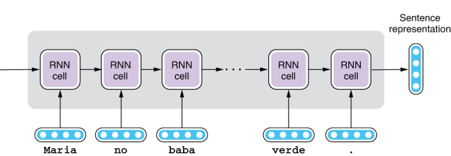
Figure 6.8 Encoder of a Seq2Seq model

Unlike sequential-labeling models, we need only the final hidden state of an RNN, which is then passed to the decoder to generate the target sentence. You can also use a multilayer RNN as an encoder, in which case the sentence representation is the concatenation of the output of each layer, as illustrated in figure 6.9.

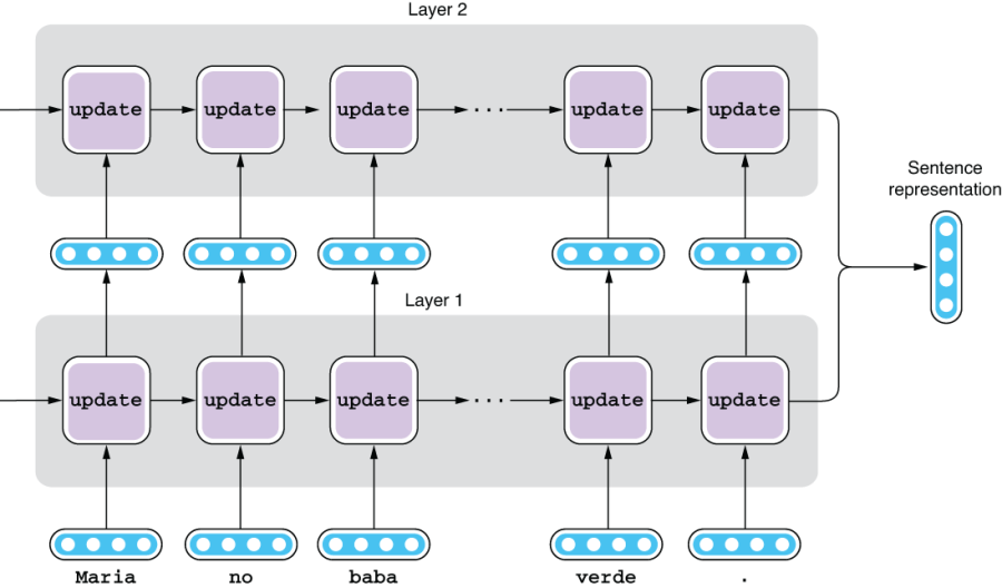
Figure 6.9 Using a multilayer RNN as an encoder

Similarly, you can use a bidirectional (or even a bidirectional multilayer) RNN as an encoder. The final sentence representation is a concatenation of the output of the forward and the backward layers, as shown in figure 6.10.

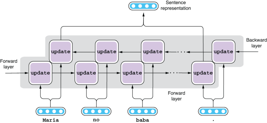
Figure 6.10 Using a bidirectional RNN as an encoder

NOTE This is a small detail, but remember that an LSTM cell produces two types of output: the cell state and the hidden state (see section 4.2.2 for review). When using LSTM for encoding a sequence, we usually just use the final hidden state while discarding the cell state. Think of the cell state as something like a temporary loop variable used for computing the final outcome (the hidden state). See figure 6.11 for an illustration.

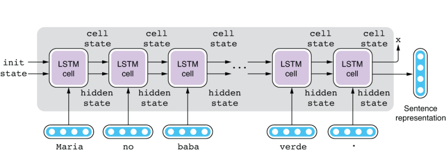
Figure 6.11 An encoder using LSTM cells

6.4.2 Decoder

Likewise, the decoder of a Seq2Seq model is similar to the language model we covered in chapter 5. In fact, they are identical except for one crucial difference—a decoder takes an input from the encoder. The language models we covered in chapter 5 are called unconditional language models because they generate language without any input or precondition. On the other hand, language models that generate language based on some input (condition) are called conditional language models. A Seq2Seq decoder is one type of conditional language model, where the condition is the sentence representation produced by the encoder. See figure 6.12 for an illustration of how a Seq2Seq decoder works.

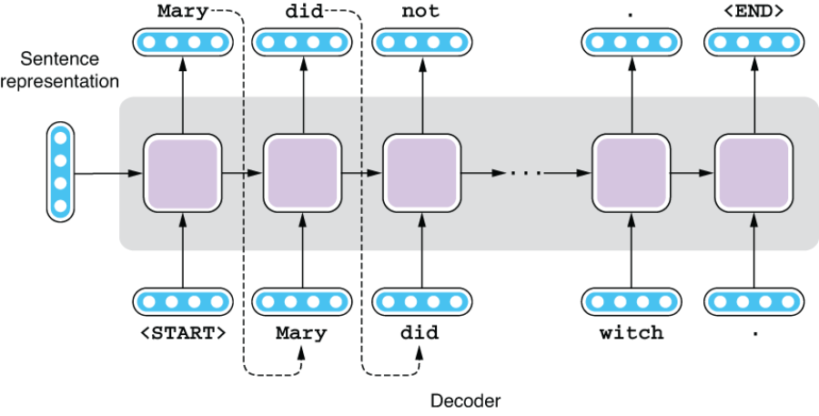
Figure 6.12 A decoder of a Seq2Seq model

Just as with language models, Seq2Seq decoders generate text from left to right. Like the encoder, you can use an RNN to do this. A decoder can also be a multilayer RNN. However, a decoder cannot be bidirectional—you cannot generate a sentence from both sides. As was mentioned in chapter 5, models that operate on the past sequence they produced are called autoregressive models.

How the decoder behaves is a bit different between the training and the prediction stages. Let’s see how it is trained first. At the training stage, we know exactly how the source sentence should be translated into the target sentence. In other words, we know exactly what the decoder should produce, word by word. Because of this, decoders are trained in a similar way to how sequential-labeling models are trained (see chapter 5).

First, the decoder is fed the sentence representation produced by the encoder and a special token <START>, which indicates the start of a sentence. The first RNN cell processes these two inputs and produces the first hidden state. The hidden state vector is fed to a linear layer that shrinks or expands this vector to match the size of the vocabulary. The resulting vector then goes through softmax, which converts it to a probability distribution. This distribution dictates how likely each word in the vocabulary is to come next.

Then, this is where the training happens. If the input is “Maria no daba una bofetada a la bruja verde,” then we would like the decoder to produce its English equivalent: “Mary did not slap the green witch.” This means that we would like to maximize the probability that the first RNN cell generates “Mary” given the input sentence. This is a multiclass classification problem we have seen many times so far in this book—word embeddings (chapter 3), sentence classification (chapter 4), and sequential labeling (chapter 5). You use the cross-entropy loss to measure how far apart the desired outcome is from the actual output of your network. If the probability for “Mary” is large, then good—the network incurs a small loss. On the other hand, if the probability for “Mary” is small, then the network incurs a large loss, which encourages the optimization algorithm to change the parameters (magic constants) by a large amount.

Then, we move on to the next cell. The next cell receives the hidden state computed by the first cell and the word “Mary,” regardless of what the first cell generated. Instead of feeding the token generated by the previous cell, as we did when generating text using a language model, we constrain the input to the decoder so that it won’t “go astray.” The second cell produces the hidden state based on these two inputs, which is then used to compute the probability distribution for the second word. We compute the cross-entropy loss by comparing the distribution against the desired output “did” and move on to the next cell. We keep doing this until we reach the final token, which is <END>. The total loss for the sentence is the average of all the losses incurred for all the words in the sentence, as shown in figure 6.13.

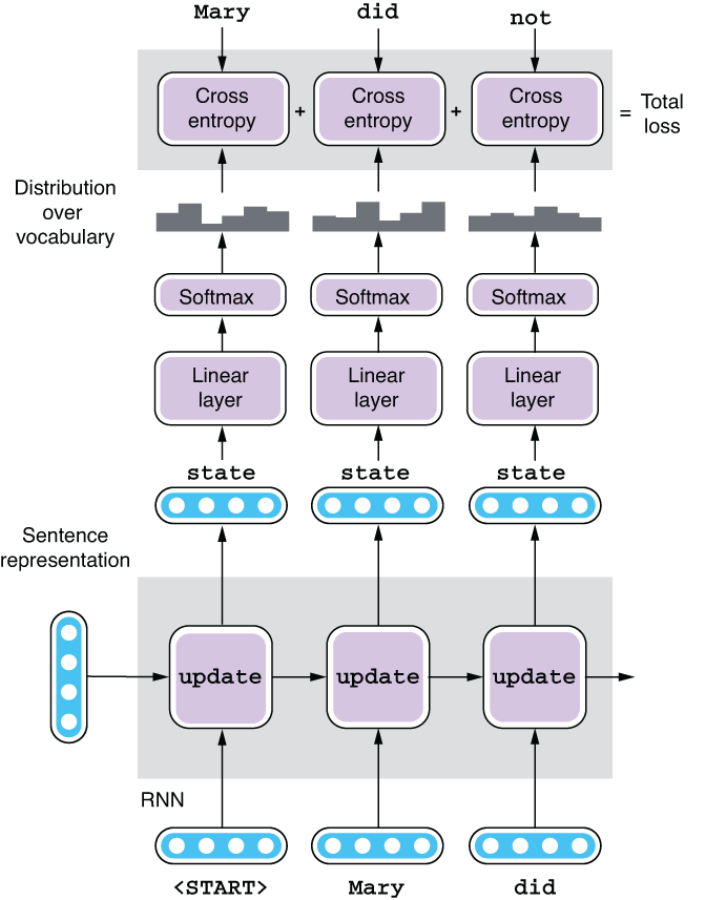
Figure 6.13 Training a Seq2Seq decoder

Finally, the loss computed this way is used to adjust the model parameters of the decoder, so that it can generate the desired output the next time around. Note that the parameters of the encoder are also adjusted in this process, because the loss propagates all the way back to the encoder through the sentence representation. If the sentence representation produced by the encoder is not good, the decoder won’t be able to produce high-quality target sentences no matter how hard it tries.

6.4.3 Greedy decoding

Now let’s look at how the decoder behaves at the prediction stage, where a source sentence is given to the network, but we don’t know what the correct translation should be. At this stage, a decoder behaves a lot like the language models we discussed in chapter 5. It is fed the sentence representation produced by the encoder, as well as a special token <START>, which indicates the start of a sentence. The first RNN cell processes these two inputs and produces the first hidden state, which is then fed to the linear layer and the softmax layer to produce the probability distribution over the target vocabulary. Here comes the key part—unlike the training phase, you don’t know the correct word to come next, so you have multiple options. You can choose any random word that has a reasonably high probability (say, “dog”), but probably the best you can do is pick the word whose probability is the highest (you are lucky if it’s “Mary”). The MT system produces the word that was just picked and then feeds it to the next RNN cell. This is repeated until the special token <END> is encountered. Figure 6.14 illustrates this process.

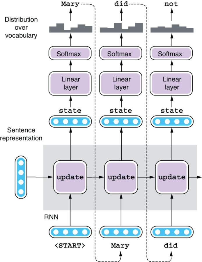
Figure 6.14 A prediction using a Seq2Seq decoder

OK, so are we all good, then? Can we move on to evaluating our MT system, because it is doing everything it can to produce the best possible translation? Not so fast—many things could go wrong by decoding the target sentence in this manner.

First of all, the goal of MT decoding is to maximize the probability of the target sentence as a whole, not just individual words. This is exactly what you trained the network to do—to produce the largest probability for correct sentences. However, the way words are picked at each step described earlier is to maximize the probability of that word only. In other words, this decoding process guarantees only the locally maximum probability. This type of myopic, locally optimal algorithm is called greedy in computer science, and the decoding algorithm I just explained is called greedy decoding. However, just because you are maximizing the probability of individual words at each step doesn’t mean you are maximizing the probability of the whole sentence. Greedy algorithms, in general, are not guaranteed to produce the globally optimal solution, and using greedy decoding can leave you stuck with suboptimal translations. This is not very intuitive to understand, so let me use a simple example to illustrate this.

When you are picking words at each timestep, you have multiple words to pick from. You pick one of them and move on to the next RNN cell, which produces another set of possible words to pick from, depending on the word you picked previously. This can be represented using a tree structure like the one shown in figure 6.15. The diagram shows how the word you pick at one timestep (e.g., “did”) branches out to another set of possible words (“you” and “not”) to pick from at the next timestep.

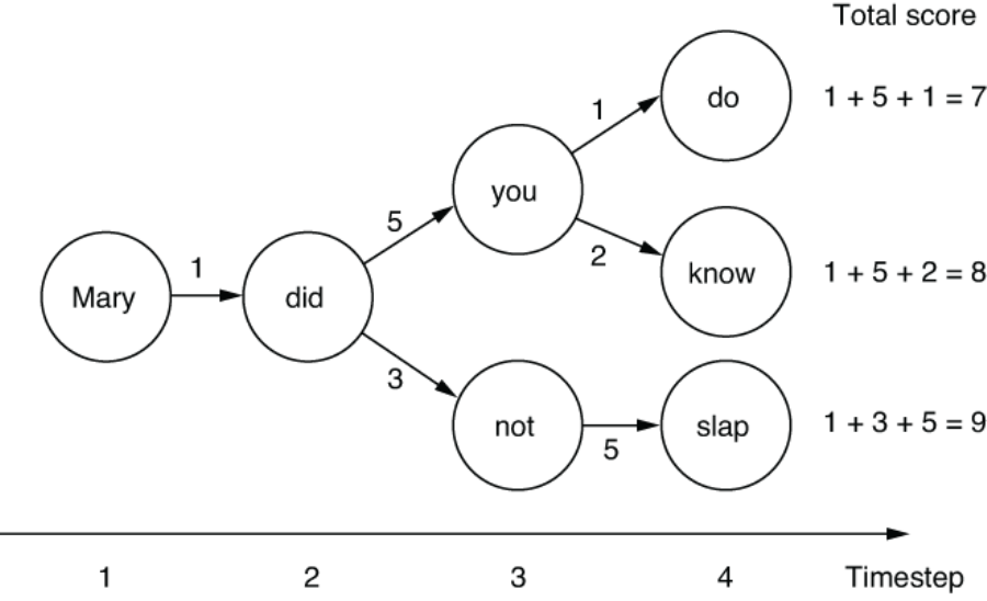
Figure 6.15 A decoding decision tree

Each transition from word to word is labeled with a score, which corresponds to how large the probability of choosing that transition is. Your goal here is to maximize the total sum of the scores when you traverse one path from timestep 1 to 4. Mathematically, probabilities are real numbers between 0 to 1, and you should multiply (instead of add) each probability to get the total, but I’m simplifying things here. For example, if you go from “Mary” to “did,” then on to “you” and “do,” you just generated a sentence “Mary did you do” and the total score is 1 + 5 + 1 = 7.

The greedy decoder we saw earlier will face two choices after it generates “did” at timestep 2: either generate “you” with a score of 5 or “not” with a score of 3. Because all it does is pick the one with the highest score, it will pick “you” and move on. Then it will face another branch after timestep 3—generating “do” with a score of 1 or generating “know” with a score of 2. Again, it will pick the largest score, and you will end up with the translation “Mary did you know” whose score is 1+ 5 + 1 = 8.

This is not a bad result. At least, it is not as bad as the first path, which sums up to a score of 7. By picking the maximum score at each branch, you are making sure that your final result is at least decent. However, what if you picked “not” at timestep 3? At first glance, this doesn’t seem like a good idea, because the score you get is only 3, which is smaller than you’d get by taking the other path, 5. But at the next timestep, by generating “slap,” you get a score of 5. In retrospect, this was the right thing to do—in total, you get 1 + 3 + 5 = 9, which is larger than any scores you’d get by taking the other “you” path. By sacrificing short-term rewards, you are able to gain even larger rewards in the long run. But due to the myopic nature of the greedy decoder, it will never choose this path—it can’t backtrack and change its mind once it’s taken one branch over another.

Choosing which way to go to maximize the total score seems easy if you look at the toy example in figure 6.15, but in reality, you can’t “foresee” the future—if you are at timestep t, you can’t predict what will happen at timestep t + 1 and onward, until you actually choose one word and feed it to the RNN. But the path that maximizes the individual probability is not necessarily the optimal solution. You just can’t try every possible path and see what score you’d get, either, because the vocabulary usually contains tens of thousands of unique words, meaning the number of possible paths is exponentially large.

The sad truth is that you can’t realistically expect to find the optimal path that maximizes the probability for the entire sentence within a reasonable amount of time. But you can avoid being stuck (or at least, make it less likely to be stuck) with a suboptimal solution, which is what the beam search decoder does.

6.4.4 Beam search decoding

Let’s think what you would do if you were in the same situation. Let’s use an analogy and say you are a college sophomore and need to decide which major to pursue by the end of the school year. Your goal is to maximize the total amount of income (or happiness or whatever thing you care about) over the course of your lifetime, but you don’t know which major is the best for this. You can’t simply try every possible major and see what happens after a couple of years—there are too many majors and you can’t go back in time. Also, just because some particular majors look appealing in the short run (e.g., choosing an economics major may lead to some good internship opportunities at large investment banks) doesn’t mean that path is the best in the long run (see what happened in 2008).

In such a situation, one thing you could do is to hedge your bet by pursuing more than one major (as a double major or a minor) at the same time instead of committing 100% to one particular major. After a couple of years, if the situation is more different than you had imagined, you can still change your mind and pursue another option, which is not possible if you choose your major greedily (i.e., based only on the short-term prospects).

The main idea of beam search decoding is similar to this—instead of committing to one path, it purses multiple paths (called hypotheses) at the same time. In this way, you leave some room for “dark horses,” that is, hypotheses that had low scores at first but may prove promising later. Let’s see this in action using the example in figure 6.16, a slightly modified version of figure 6.15.

The key idea of beam search decoding is to use a beam (figure 6.16 bottom), which you can think of as some sort of buffer that can retain multiple hypotheses at the same time. The size of the beam, that is, the number of hypotheses it can retain, is called the beam width. Let’s use a beam of size 2 and see what happens. Initially, your first hypothesis consists of only one word, “Mary,” and a score of 0. When you move on to the next word, the word you chose is appended to the hypothesis, and the score is incremented by the score of the path you have just taken. For example, when you move on to “did,” it will make a new hypothesis consisting of “Mary did” and a score of 1.

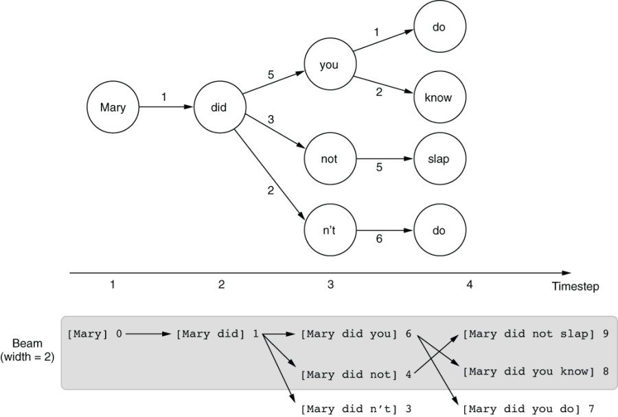
Figure 6.16 Beam search decoding

If you have multiple words to choose from at any particular timestep, a hypothesis can spawn multiple child hypotheses. At timestep 2, you have three different choices—“you,” “not,” and “n’t”—which generate three new child hypotheses: [Mary did you] (6), [Mary did not] (4), and [Mary did n’t] (3). And here’s the key part of beam search decoding: because there’s only so much room in the beam, any hypotheses that are not good enough fall off of the beam after sorting them by their scores. Because the beam can hold up to only two hypotheses in this example, anything except the top two gets kicked out of the beam, which leaves [Mary did you] (6) and [Mary did not] (4).

At timestep 3, each remaining hypothesis can spawn up to two child hypotheses. The first one ([Mary did you] (6)) will generate [Mary did you know] (8) and [Mary did you do] (7), whereas the second one ([Mary did not] (4)) turns into [Mary did not slap] (9). These three hypotheses are sorted by their scores, and the best two will be returned as the result of the beam search decoding.

Congratulations—now your algorithm was able to find the path that maximizes the total sum of the scores. By considering multiple hypotheses at the same time, beam search decoding can increase the chance that you will find better solutions. However, it is never perfect—notice that an equally good path [Mary did n’t do] with a score of 9 fell out of the beam as early as timestep 3. To “rescue” it, you’d need to increase the beam width to 3 or larger. In general, the larger the beam width, the higher the expected quality of the translation results will be. However, there’s a tradeoff: because the computer needs to consider multiple hypotheses, it will be linearly slower as the beam width increases.

In Fairseq, you can use the —beam option to change the beam size. In the example in section 6.3.3, I used —beam 5 to use a beam width of 5. You were already using beam search without noticing. If you invoke the same command with —beam 1, which means you are using greedy decoding instead of a beam search, you may get slightly different results. When I tried this, I got almost the same results except the last one: “counts, please,” which is not a great translation for “La cuenta, por favor.” This means using a beam search indeed helps improve the translation quality!

6.5 Evaluating translation systems

In this section, I’d like to briefly touch on the topic of evaluating machine translation systems. Accurately evaluating MT systems is an important topic, both in theory and practice.

6.5.1 Human evaluation

The simplest and the most accurate way to evaluate MT systems’ output is to use human evaluation. After all, language is translated for humans. Translations that are deemed good by humans should be good.

As mentioned previously, we have a few considerations for what makes a translation good. There are two most important and commonly used concepts for this—adequacy (also called fidelity) and fluency (also closely related to intelligibility). Adequacy is the degree to which the information in the source sentence is reflected in the translation. If you can reconstruct a lot of information expressed by the source sentence by reading its translation, then the translation has high adequacy. Fluency is, on the other hand, how natural the translation is in the target language. If you are translating into English, for example, “Mary did not slap the green witch” is a fluent translation, whereas “Mary no had a hit with witch, green” is not, although both translations are almost equally adequate. Note that these two aspects are somewhat independent—you can think of a translation that is fluent but not adequate (e.g., “Mary saw a witch in the forest” is a perfectly fluent but inadequate translation) and vice versa, like the earlier example. MT systems that produce output that is both adequate and fluent are desirable.

An MT system is usually evaluated by presenting its translations to human annotators and having them judge its output on a 5- or 7-point scale for each aspect. Fluency is easier to judge because it requires only monolingual speakers of the target sentence, whereas adequacy requires bilingual speakers of both the source and target languages.

6.5.2 Automatic evaluation

Although human evaluation gives the most accurate assessment to MT systems’ quality, it’s not always feasible. In most cases, you cannot afford to hire human evaluators to assess an MT system’s output every time you need it. If you are dealing with language pairs that are not common, you might not be able to find bilingual speakers for evaluating adequacy at all.

But more importantly, you need to constantly evaluate and monitor an MT system’s quality when you are developing one. For example, if you use a Seq2Seq model to train an NMT system, you need to reevaluate its performance every time you adjust one of the hyperparameters. Otherwise, you wouldn’t know whether your change has a good or bad effect on its final performance. Even worse, if you were to do something like early stopping (see section 6.3.2) to determine when to stop the training process, you would need to evaluate its performance after every epoch. You can’t possibly hire somebody and have them evaluate your intermediate models at each epoch—that would be a terribly slow way to develop an MT system. It’s also a huge waste of time, because the output of initial models is largely garbage and does not warrant human evaluation. A large amount of correlation exists between the outputs of intermediate models, and human evaluators would be spending a lot of time evaluating very similar, if not identical, sentences.

For this reason, it’d be desirable if we could use some automatic way to assess translation quality. The way this works is similar to some automatic metrics for other NLP tasks that we saw earlier, such as accuracy, precision, recall, and F1-measure for classification. The idea is to create the desirable output for each input instance in advance and compare a system’s output against it. This is usually done by preparing a set of human-created translations called reference for each source sentence and calculating some sort of similarity between the reference and a system’s output. Once you create the reference and define the metric, you can automatically evaluate translation quality as many times as you want.

One of the simplest ways to compute the similarity between the reference and a system output is to use the word error rate (WER). WER reflects how many errors the system made compared to the reference, measured by the relative number of insertions, deletions, and substitutions. The concept is similar to the edit distance, except that WER is counted for words, not characters. For example, when the reference sentence is “Mary did not slap the green witch” and a system translation is “Mary did hit the green wicked witch,” you need three “edits” to match the latter to the former—insert “not,” replace “hit” with “slap,” and delete “wicked.” If you divide three by the length of the reference (= 7), it’s your WER (= 3/7, or 0.43). The lower the WER, the better the quality of your translation.

Although WER is simple and easy to compute, it is not widely used for evaluating MT systems nowadays. One reason is related to multiple references. There may be multiple, equally valid translations for a single source sentence, but it is not clear how to apply WER when there are multiple references. A slightly more advanced and by far the most commonly used metric for automatic evaluation in MT is BLEU (bilingual evaluation understudy). BLEU solves the problem of multiple references by using modified precision. I’ll illustrate this next using a simple example.

In the following table, we are evaluating a candidate (a system’s output) “the the the the the the the” (which is, by the way, a terrible translation) against two references: “the cat is on the mat” and “there is a cat on the mat.” The basic idea of BLEU is to calculate the precision of all unique words in the candidate. Because there’s only one unique word in the candidate, “the,” if you calculate its precision, it will automatically become the candidate’s score, which is 1, or 100%. But there seems to be something wrong about this.

Because only two “thes” exist in the references, the spurious “thes” generated by the system shouldn’t count toward the precision. In other words, we should treat them as false positives. We can do this by capping the denominator of precision by the maximum number of occurrences of that word in any of the references. Because it’s 2 in this case (in reference 1), its modified precision will be 2/7, or about 29%. In practice, BLEU uses not only unique words (i.e., unigrams) but also all unique sequences of words (n-grams) up to a length of 4 in the candidate and the references.

However, we can game this metric in another way—because it’s based on precision, not on recall, an MT system can easily obtain high scores by producing very few words that the system is confident about. In the previous example, you can simply produce “cat” (or even more simply, “the”), and the BLEU score will be 100%, which is obviously not a good translation. BLEU solves this issue by introducing the brevity penalty, which discounts the score if the candidate is shorter than the references.

Development of accurate automatic metrics has been an active research area. Many new metrics are proposed and used to address the shortcomings of BLEU. We barely scratched the surface in this section. Although new metrics show higher correlations with human evaluations and are claimed to be better, BLEU is still by far the most widely used metric, mainly due to its simplicity and long tradition.

6.6 Case study: Building a chatbot

In this section, I’m going to go over another application of a Seq2Seq model—a chatbot, which is an NLP application with which you can have a conversation. We are going to build a very simple yet functional chatbot using a Seq2Seq model and discuss techniques and challenges in building intelligent agents.

6.6.1 Introducing dialogue systems

I briefly touched upon dialogue systems in section 1.2.1. To recap, two main types of dialogue systems exist: task-oriented and chatbots. Although task-oriented dialogue systems are used to achieve some specific goals, such as making a reservation at a restaurant and obtaining some information, chatbots are used to have conversations with humans. Conversational technologies are currently a hot topic among NLP practitioners, due to the success and proliferation of commercial conversational AI systems such as Amazon Alexa, Apple Siri, and Google Assistant.

You may not have a clue as to how we can get started with building an NLP application that can have conversations. How can we build something “intelligent” that “thinks” so that it can generate meaningful responses to human input? This seems farfetched and difficult. But if you step back and look at a typical conversation we have with other people, how much of it is actually “intelligent?” If you are like most of us, a large fraction of the conversation you are having is autopilot: “How are you?” “I’m doing good, thanks” “Have a good day” “You, too!” and so on. You may also have a set of “template” responses to a lot of everyday questions such as “What do you do?” and “Where are you from?” These questions can be answered just by looking at the input. Even more complex questions like “What’s your favorite restaurant in X?” (where X is the name of a neighborhood in your city) and “Did you see any Y movies lately?” (where Y is a genre) can be answered just by “pattern matching” and retrieving relevant information from your memory.

If you think of a conversation as a set of “turns” where the response is generated by pattern matching against the previous utterance, this starts to look a lot like a typical NLP problem. In particular, if you regard dialogues as a problem where an NLP system is simply converting your question to its response, this is exactly where we can apply the Seq2Seq models we covered in this chapter so far. We can treat the previous (human’s) utterance as a foreign sentence and have the chatbot “translate” it into another language. Even though these two languages are both English in this case, it is a common practice in NLP to treat the input and the output as two different languages and apply a Seq2Seq model to them, including summarization (longer text to a shorter one) and grammatical error correction (text with errors to one without).

6.6.2 Preparing a dataset

In this case study, we are going to use The Self-dialogue Corpus (https://github.com/jfainberg/self_dialogue_corpus), a collection of 24,165 conversations. What’s special about this dataset is that these conversations are not actual ones between two people, but fictitious ones written by one person who plays both sides. You could use several conversation datasets for text-based chatbots (e.g., the OpenSubtitles dataset, http://opus.nlpl.eu/OpenSubtitles-v2018.php), but these datasets are often noisy and often contain obscenities. By collecting made-up conversations instead, the Self-dialogue Corpus improves the quality for half the original cost (because you need only one person versus two people!).

The same as earlier, I tokenized and converted the corpus into a format that is interpretable by Fairseq. You can obtain the converted dataset as follows:

$ mkdir -p data/chatbot
$ wget https://realworldnlpbook.s3.amazonaws.com/data/chatbot/selfdialog.zip
$ unzip selfdialog.zip -d data/chatbot

You can use the following combination of the paste command (to stitch files horizontally) and the head command to peek at the beginning of the training portion. Note that we are using fr (for “foreign,” not “French”) to denote the “language” we are translating from:

$ paste data/chatbot/selfdialog.train.tok.fr data/chatbot/selfdialog.train.tok.en | head 
...
Have you played in a band ?    What type of band ?
What type of band ?    A rock and roll band .
A rock and roll band .    Sure , I played in one for years .
Sure , I played in one for years .    No kidding ?
No kidding ?    I played in rock love love .
I played in rock love love .    You played local ?
You played local ?    Yes
Yes    Would you play again ?
Would you play again ?    Why ?
...

As you can see, each line consists of an utterance (on the left) and a response to it (on the right). Notice that this dataset has the same structure as the Spanish-English parallel corpus we used in section 6.3.1. The next step is to run the fairseq-preprocess command to convert it to a binary format as follows:

$ fairseq-preprocess 
    --source-lang fr 
    --target-lang en 
    --trainpref data/chatbot/selfdialog.train.tok 
    --validpref data/chatbot/selfdialog.valid.tok 
    --destdir data/chatbot-bin 
    --thresholdsrc 3 
    --thresholdtgt 3

Again, this is similar to what we ran for the Spanish translator example. Just pay attention to what you specify as the source language—we are using fr instead of es here.

6.6.3 Training and running a chatbot

Now that the training data for the chatbot is ready, let’s train a Seq2Seq model from this data. You can invoke the fairseq-train command with almost identical parameters to the last time, as shown next:

$ fairseq-train 
    data/chatbot-bin 
    --arch lstm 
    --share-decoder-input-output-embed 
    --optimizer adam 
    --lr 1.0e-3 
    --max-tokens 4096 
    --save-dir data/chatbot-ckpt

As previously, pay attention to how the validation loss changes every epoch. When I tried this, the validation loss decreased for about five epochs but then started to slowly creep back up. Feel free to stop the training command by pressing Ctrl + C after you observe the validation loss leveling out. Fairseq will automatically save the best model (measured by the validation loss) to checkpoint_best.pt.

Finally, you can run the chatbot model by invoking the fairseq-interactive command, as shown here:

$ fairseq-interactive 
    data/chatbot-bin 
    --path data/chatbot-ckpt/checkpoint_best.pt 
    --beam 5 
    --source-lang fr 
    --target-lang en

As with the previous example, you can type your source sentences and have a conversion with your chatbot by having them “translate” to another language! Here’s part of a conversation that I had with the model that I trained (I added boldface for clarity). Again, your results might be different:

Hi !
S-0     Hi !
H-0     -1.011711835861206      Hey .
P-0     -0.6860 -2.1352 -0.2140
How are you ?
S-1     How are you ?
H-1     -0.6552960276603699     Doing good , you ?
P-1     -0.6472 -0.8651 -1.0960 -0.9257 -0.3337 -0.0640
Good .
S-2     Good .
H-2     -0.8540937900543213     Do you have a favorite team ?
P-2     -2.3027 -0.0550 -1.7088 -0.4403 -0.1763 -2.0262 -0.1150 -0.0085
Yeah I like the Seahawks .
S-3     Yeah I like the Seahawks .
H-3     -0.6036218404769897     Do you have a favorite team ?
P-3     -2.7614 -0.0525 -1.0905 -0.3178 -0.3213 -0.1049 -0.1701 -0.0106
How about you ?
S-4     How about you ?
H-4     -1.2329542636871338     I 'm a big fan of them .
P-4     -0.7648 -1.8435 -1.6808 -1.2868 -0.2102 -0.1362 -3.5273 -1.0031 -0.6438
What 's your favorite movie ?
S-5     What 's your favorite movie ?
H-5     -0.8238655924797058     Oh , that 's a tough one . I 'd have to say Ghost Busters .
P-5     -3.2622 -0.3213 -1.4815 -0.1012 -0.3417 -0.3069 -0.2432 -0.6954 -1.0858 -2.3246 -0.4296 -0.0039 -0.0905 -2.6429 -0.1676 -0.3853 -0.1221
Oh yeah , I like that movie too .
S-6     Oh yeah , I like that movie too .
H-6     -1.0659444332122803     Yeah , that 's a good one .
P-6     -2.0782 -0.1724 -2.5089 -0.9560 -1.5034 -0.9040 -0.4471 -0.5435 -0.4801

In this example, the conversation looks natural. Because the Self-dialogue Corpus is built by restricting the set of possible conversation topics, the conversation is more likely to go smoothly if you stay on such topics (movie, sports, music, and so on).

However, as soon as you start talking about unfamiliar topics, the chatbot loses its confidence in its answers, as shown next:

What 's your name ?
S-0     What 's your name ?
H-0     -0.9807574152946472     I do n't know , but I do n't think I 've                           heard of them .
P-0     -1.4680 -2.2938 -0.0635 -1.0242 -1.2039 -0.5201 -0.3381 -2.2612 -0.1665 -1.6033 -0.6112 -1.5515 -0.8739 -0.8453 -1.0143 -0.4702 -0.3637
What do you do ?
S-1     What do you do ?
H-1     -1.170507788658142      I do n't know .
P-1     -0.9807 -2.1846 -0.3276 -0.9733 -1.3650 -1.1919
Are you a student ?
S-2     Are you a student ?
H-2     -0.9505285024642944     I 'm not sure .
P-2     -1.5676 -1.5270 -0.6944 -0.2493 -0.8445 -0.8204

This is a well-known phenomenon—a simple Seq2Seq-based chatbot quickly regresses to producing cookie-cutter answers such as “I don’t know” and “I’m not sure” whenever asked about something it’s not familiar with. This has to do with the way we trained this chatbot. Because we trained the model so that it minimizes the loss in the training data, the best strategy it can take to reduce the loss is to produce something applicable to as many input sentences as possible. Very generic phrases such as “I don’t know” can be an answer for many questions, so it’s a great way to play it safe and reduce the loss!

6.6.4 Next steps

Although our chatbot can produce realistic-looking responses for many inputs, it’s far from perfect. One issue that it’s not great at dealing with is proper nouns. You can see this when you ask questions that solicit specific answers, like the following:

What 's your favorite show ?
S-0     What 's your favorite show ?
H-0     -0.9829921722412109     I would have to say <unk> .
P-0     -0.8807 -2.2181 -0.4752 -0.0093 -0.0673 -2.9091 -0.9338 -0.3705

Here <unk> is the catch-all special symbol for unknown words. The chatbot is trying to answer something, but that something occurs too infrequently in the training data to be treated as an independent word. This is an issue seen in simple NMT systems in general. Because the models need to cram everything about a word in a 200-something-dimensional vector of numbers, many details and distinctions between similar words are sacrificed. Imagine compressing all the information about all the restaurants in your city into a 200-dimensional vector!

Also, the chatbot we trained doesn’t have any “memory” or any notion of context whatsoever. You can test this by asking a series of related questions as follows:

Do you like Mexican food ?
S-0     Do you like Mexican food ?
H-0     -0.805641770362854      Yes I do .
P-0     -1.0476 -1.1101 -0.6642 -0.6651 -0.5411
Why do you like it ?
S-1     Why do you like it ?
H-1     -1.2453081607818604     I think it 's a great movie .
P-1     -0.7999 -2.1023 -0.7766 -0.7130 -1.4816 -2.2745 -1.5750 -1.0524 -0.4324

In the second question, the chatbot is having difficulties understanding the context and produces a completely irrelevant response. To answer such questions correctly, the model needs to understand that the pronoun “it” refers to a previous noun, namely, “Mexican food” in this case. The task where NLP systems resolve which mentions refer to which entities in the real world is called coreference resolution. The system also needs to maintain some type of memory to keep track of what was discussed so far in the dialogue.

Finally, the simple Seq2Seq models we discussed in this chapter are not great at dealing with long sentences. If you look back at figure 6.2, you’ll understand why—the model reads the input sentence using an RNN and represents everything about the sentence using a fixed-length sentence representation vector and then generates the target sentence from that vector. It doesn’t matter whether the input is “Hi!” or “The quick brown fox jumped over the lazy dog.” The sentence representation becomes a bottleneck, especially for longer input. Because of this, neural MT models couldn’t beat traditional phrase-based statistical MT models until around 2015, when a mechanism called attention was invented to tackle this very problem. We’ll discuss attention in detail in chapter 8.

Summary

• Sequence-to-sequence (Seq2Seq) models transform one sequence into another using an encoder and a decoder.

• You can use the fairseq framework to build a working MT system within an hour.

• A Seq2Seq model uses a decoding algorithm to generate the target sequence. Greedy decoding maximizes the probability at each step, whereas beam search tries to find better solutions by considering multiple hypotheses at once.

• A metric called BLEU is commonly used for automatically evaluating MT systems.

• A simple chatbot can be built by using a Seq2Seq model and a conversation dataset.