
1
Basic Reliability Concepts and Models
1.1 Introduction
Reliability is a statistical approach to describing the dependability and the ability of a system or component to function under stated conditions for a specified period of time in the presence of uncertainty. In this chapter, we provide the statistical definition of reliability, and further introduce the concepts of failure rate, hazard rate, bathtub curve, and their relation with the reliability function. We also present several lifetime metrics that are commonly used in industry, such as mean time between failures, mean time to failure, and mean time to repair. For repairable systems, failure intensity rate, mean time between replacements and system availability are the primary reliability measures. The role of line replaceable unit and consumable items in the repairable system is also elaborated. Finally, we discuss the parametric models commonly used for lifetime prediction and failure analysis, which include Bernoulli, binomial, Poisson, exponential, Weibull, normal, lognormal, and gamma distributions. The chapter is concluded with the reliability inference using Bayesian theory and Markov models.
1.2 Reliability Definition and Hazard Rate
1.2.1 Managing Reliability for Product Lifecycle
Reliability engineering is an interdisciplinary field that studies, evaluates, and manages the lifetime performance of components and systems, such as automobile, wind turbines (WTs), aircraft, Internet, medical devices, power system, and radars, among many others (Blischke and Murthy 2000; Chowdhury and Koval 2009). These systems and equipment are widely used in commercial and defense sectors, ranging from manufacturing, energy, transportation, healthcare, communication, and military operations.
The lifecycle of a product typically consist of five phases: design/development, new product introduction, volume shipment, market saturation, and phase‐out. Figure 1.1 depicts the inter‐dependency of five phases. Reliability plays a dual role across the lifecycle of a product: reliability as engineering (RAE) and reliability as services (RASs). RAE encompasses reliability design, reliability growth planning, and warranty and maintenance. RAS concentrates on the planning and management of a repairable inventory system, spare parts supply, and recycling and remanufacturing of end‐of‐life products. RAE and RAS have been studied intensively, but often separately in reliability engineering and operations management communities. The merge of RAE and RAS is driven primarily by the intense global competition, compressed product design cycle, supply chain volatility, environmental sustainability, and changing customer needs. There is a growing trend that RAE and RAS will be seamlessly integrated under the so‐called product‐service system, which offers a bundled reliability solution to the customers. This book aims to present an integrated framework that allows the product manufacturer to develop and market reliable products with low cost from a product's lifecycle perspective.

Figure 1.1The role of reliability in the lifecycle of a product.
In many industries, reliability engineers are affiliated with a quality control group, engineering design team, supply chain logistics, and after‐sales service group. Due to the complexity of a product, reliability engineers often work in a cross‐functional setting in terms of defining the product reliability goal, advising corrective actions, and planning spare parts. When a new product is introduced to the market, the initial reliability could be far below the design target due to infant mortality, variable usage, latent failures, and other uncertainties. Reliability engineers must work with the hardware and software engineers, component purchasing group, manufacturing and operations department, field support and repair technicians, logistics and inventory planners, and marketing team to identify and eliminate the key root causes in a timely, yet cost‐effective manner. Hence, a reliability engineer requires a wide array of skill sets ranging from engineering, physics, mathematics, statistics, and operations research to business management. Last but not the least, a reliability engineer must possess strong communication capability in order to lead initiatives for corrective actions, resolve conflicting goals among different organization units, and make valuable contributions to product design, volume production, and after‐sales support.
1.2.2 Reliability Is a Probabilistic Measure
Reliability is defined as the ability of a system or component to perform its required functions under stated conditions for a specified period of time (Elsayed 2012; O'Connor 2012). It is often measured as a probability of failure or a possibility of availability. Let T be a non‐negative random variable representing the lifetime of a system or component. Then the reliability function, denoted as R(t), is expressed as
It is the probability that T exceeds an expected lifetime t which is typically specified by the manufacturer or customer. For example, in the renewable energy industry, the owner of the solar park would like to know the reliability of the photovoltaic (PV) system at the end of t = 20 years. Then the reliability of the solar photovoltaic system can be expressed as R(20) = P {T > 20}. As another example, as more electric vehicles (EVs) enter the market, the consumers are concerned about the reliability of the battery once the cumulative mileage reaches 100 000 km. In that case, t = 100 000 km and the reliability of the EV battery can be expressed as R(100 000) = P {T > 100 000}. Depending on the actual usage profile, the lifetime T can stand for a product's calendar age, mileage, or charge–recharge cycles (e.g. EV battery). The key elements in the definition of Eq. 1.2.1 are highlighted below.
- Reliability is predicted based on “intended function” or “operation” without failure. However, if individual parts are good but the system as a whole does not achieve the intended performance, then it is still classified as a failure. For instance, a solar photovoltaic system has no power output in the night. Therefore, the reliability of energy supply is zero even if solar panels and DC–AC inverters are good.
- Reliability is restricted to operation under explicitly defined conditions. It is virtually impossible to design a system for unlimited conditions. An EV will have different operating conditions than a battery‐powered golf car even if they are powered by the same type of battery. The operating condition and surrounding environment must be addressed during design and testing of a new product.
- Reliability applies to a specified period of time. This means that any system eventually will fail. Reliability engineering ensures that the system with a specified chance will operate without failure before time t.
The relationship between the time‐to‐failure distribution F(t) and the reliability function R(t) is governed by
In statistics, F(t) is also referred to as the cumulative distribution function (CDF). Let f(t) be the probability density function (PDF); the relation between R(t) and f(t) is given as follows:

1.2.3 Failure Rate and Hazard Rate Function
Let t be the start of an interval and Δt be the length of the interval. Given that the system is functioning at time t, the probability that the system will fail in the interval of [t, t + Δt] is
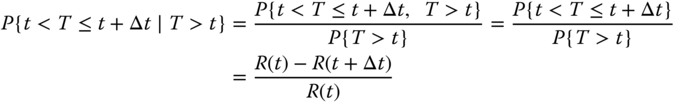
The result is derived based on the Bayes theorem by realizing P{A, B} = P{A}, where A is the event that the system fails in the interval [t, t + Δt] and B is the event that the system survives through t.
The failure rate, denoted as z(t), is defined in a time interval [t, t + Δt] as the probability that a failure per unit time occurs in that interval given that the system has survived up to t. That is,

Although the failure rate z(t) in Eq. 1.2.5 is often thought of as the probability that a failure occurs in a specified interval like [t, t + Δt] given no failure before time t, it is indeed not a probability because z(t) can exceed 1. For instance, given R(t) = 0.5, R(t + Δt) = 0.4, and Δt = 0.1, then z(t) = 2 failures per unit time. Hence, the failure rate represents the frequency with which a system or component fails and is expressed in failures per unit time. The actual failure rate of a product or system is closely related to the operating environment and customer usage (Cai et al. 2011).
1.2.4 Bathtub Hazard Rate Curve
As the name implies, the bathtub hazard rate curve is derived from the cross‐sectional shape of a bathtub. As shown in Figure 1.2, the bathtub curve consists of three different types of hazard rate profiles: (i) early infant mortality failures when the product is initially introduced; (ii) the constant rate during its useful period; and (iii) the increasing rate of wear‐out or degradation failures as the product continues to operate at the end or beyond its design lifetime.
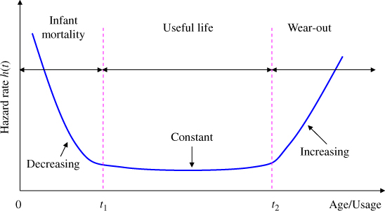
Figure 1.2Bathtub hazard rate curve.
In military and consumer electronics industries, the infant mortality is often burned out or eliminated through the so-called environmental screening process. Namely, prior to the customer shipment, the products are tested under harsher operating conditions (e.g. temperature, humidity, vibration, and electric voltage) for a designated period of time in order to filter the weak units from the product pool. This process is adopted mainly for mission or safety critical applications as it greatly reduces the possibility of occurrence of system failures in its early life. While the bathtub curve is useful, not every product or system follows a bathtub type of hazard rate profile. For example, if units are decommissioned earlier or their usage has decreased steadily during or before the onset of the wear‐out period, they will exhibit fewer failures per unit time over the chronological or calendar time (not per unit of use time) than the bathtub curve. Another case is the software products that may experience an infant mortality phase and then stabilized at a low constant hazard rate after extensive debugging and testing. This means the software product usually does not have a wear‐out phase unless the hardware that runs the software application has been changed.
1.2.5 Failure Intensity Rate
A repairable system, if it fails, can be repaired and restored to a good state. This is done by replacing failed components with good units. As time evolves, the frequency of failures may increase, decrease, or stay at a constant level depending on the maintenance policy, the reliability of existing components, and the new components used. Therefore, a system upon repair can be brought to one of the following conditions: as‐good‐as‐new, as‐good‐as‐old, and somewhere in between. The failure intensity function is a metric typically used to measure the occurrence of failures per unit time for a repairable system. A distinction shall be made between the hazard rate and the failure intensity rate. The former is used to characterize the time to the first failure of a component, while the latter deals with reoccurring failures of the same system. Hence the failure intensity rate is also referred to as the rate of occurrence of failures (ROCOFs). Let M(t) be accumulative failures (or repairs) that occurred in a repairable system during [0, t]. The ROCOF, denoted as m(t), can be estimated as
The unit of ROCOF is failures per unit time. For example, if a system failed three times in 300 days, then ROCOF = 3/300 = 0.01 failure/day. Note that failures in a repairable system may happen on different component types or on the same component types, but different items.
1.3 Mean Lifetime and Mean Residual Life
1.3.1 Mean‐Time‐to‐Failure
The mean‐time‐to‐failure (MTTF) is a quantitative metric commonly used to assess the reliability of non‐repairable systems or products. It measures the expected lifetime of a component or system before it fails. For instance, a solar photovoltaic panel is considered as a non‐repairable system with a typical MTTF between 20 and 30 years. The MTTF of a tire for commercial vehicles varies between 30 000 miles and 60 000 miles (1 mile = 1.6 km). Since these items are non‐repairable upon failure, they are either discarded or recycled for the environmental protection purpose. In industry, non‐repairable products are also called consumable items.
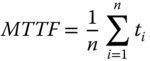
Let n be the number of non‐repairable systems operating in the field. The observed time‐to‐failure of an individual system is designated as t1, t2, …, tn. Then its MTTF can be estimated by
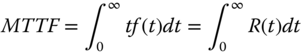
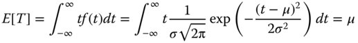
If the sample size n is large enough, the time‐to‐failure distribution for T can be inferred statistically. Then MTTF is equivalent to the expected value of T, namely
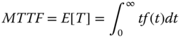
where f(t) is the PDF of the system life. MTTF can also be expressed as the integration of R(t) over [0, +∞) by performing the integration by part in Eq. 1.3.2. This results in
1.3.2 Mean‐Time‐Between‐Failures
For a repairable system, the average time between two consecutive failures is characterized by the mean‐time‐between‐failures (MTBFs). Both MTBF and MTTF measure the average uptime of a system, but MTBF is used for repairable systems as opposed to the MTTF for non‐repairable systems. For instance, tires are considered as a non‐repairable component, and their reliability performance is characterized by MTTF. However, a car installed with four tires is a repairable system, and the reliability of a car is measured by MTBF. Let t1, t2, t3,…, tn be the interarrival time between two consecutive failures. Then the MTBF of a repairable system is estimated by
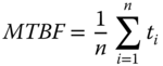
For instance, starting from day 1, a machine failed in days 9 and 35, respectively. Assume the repair time is short and negligible; then t1 = 9–0 = 9 days. As another example, after a car has run for 60 000 km, three failures have been observed. These failures correspond to one broken tire, a dead battery, and malfunction of one headlight. Then the MTBF of the car is MTBF = 60 000/3 = 20 000 km.
When estimating the MTBF, the downtime associated with waiting for repair technicians, spare parts shipping time, failure diagnostics, and administrative delay should be excluded. In other words, the MTBF only measures the average uptime when a repairable system is available for production during two consecutive failures.
1.3.3 Mean‐Time‐Between‐Replacements
For a repairable system comprised of multiple component types, the mean‐time‐between‐replacements (MTBRs) is a reliability measure associated with a specific component type. Components of different types can be classified into repairable or non‐repairable unit. For instance, an aircraft landing gear is repairable while the tires are treated as non‐repairable. If components are repairable, they are also known as a line‐replaceable unit (LRU). If components are non‐repairable, they are called a consumable part. For example, modern WTs are a repairable system, and each turbine typically comprises three blades, a main bearing, a gearbox, a generator, power electronics, and other control units. Components like the gearbox and generator are LRUs as they are repairable units. A failed generator after being fixed in the repair shop can be reused in other WTs. Turbine blades and bearings are treated as consumable parts. Upon failure, they are discarded or recycled instead of being repaired and reused.
There are two types of replacements depending on whether the component failed suddenly or has reached its scheduled maintenance age (but not failed). The latter is called a preventive replacement. Mathematically, MTBR stands for the average time between two consecutive replacements that consider both failure replacements and planned replacements. Let t1, t2, …, tn be the time‐to‐failure replacement and let τ1, τ2, …, τm be the time‐to‐planned replacement. By referring to the replacement scenarios in Figure 1.9, the MTBR of a particular component type in a repairable system can be calculated by
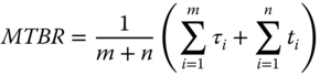

Figure 1.9Replacement scenarios for a repairable system.
In preventive maintenance, the replacement interval is often scheduled in advance with a fixed length (i.e. τi = τ for all i). If the hands‐on replacement time is short and can be ignored, the expected value of MTBR under the constant replacement interval policy can be obtained as

Note that τR(τ) captures all scheduled replacement events with fixed interval τ and ![]() stands for the failure replacements occurring prior to τ.
stands for the failure replacements occurring prior to τ.
1.3.4 Mean Residual Life
In reliability engineering, the expected additional lifetime given that a component or system has survived until time t is called the mean residual life (Gupta and Bradley 2003). Let T represent the life of a component or system. The mean residual life, denoted as L(t), is given as

where fT ∣ T ≥ t(x) is the conditional PDF given that T ≥ t. The value of L(t) can be predicted or estimated based on the historical failure data, and the result is frequently used for provisioning spare parts supply or allocating repair resources in the repair shop. The conditional PDF fT ∣ T ≥ t(x) can be expressed as the marginal PDF f(t) and reliability function R(t) as follows:

Substituting Eq. 1.3.12 into 1.3.11, the mean residual life is obtained as

1.4 System Downtime and Availability
1.4.1 Mean‐Time‐to‐Repair
Mean‐time‐to‐repair (MTTR) represents the time elapse from the moment the system is down to the moment it is resorted. MTTR encompasses the waiting time for repair technicians, the lead time of receiving spare parts, failure diagnostics time, hands‐on time for replacing any faulty parts, and other downtime associated with inspections, testing, or administrative delays. A generic MTTR estimate is given below
where
- tad
- = administrative delay
- tpt
- = lead time for receiving the spare part
- ttn
- = time for assembling the repair technician team
- tho
- = hands‐on time for replacing failed units
- tft
- = failure diagnostics and testing time
For example, a plane is grounded due to the failure of an engine. Suppose the administrative delay is two days, the lead time to receive a new engine is three days, the technicians are available after two days, the hands‐on time to replace the engine is two days, and failure diagnostics and final testing requires one day. Assume the delivery of a new engine and the dispatch of technicians occur concurrently; then MTTR = 2 + max{3, 2} + 2 + 1 = 8 days. Figure 1.10 graphically illustrates how to estimate the MTTR in this case. This example indicates that the actual MTTR can be shrunken if multiple activities can be executed concurrently. Hence Eq. 1.4.1 represents the upper bound estimate of MTTR.

Figure 1.10The MTTR of replacing an aircraft engine.
1.4.2 System Availability
Availability is the proportion of time when a system is in a functioning condition. Reliability and maintainability jointly determine the system availability. Particularly, the former determines the length of MTBF and the latter influences the MTTR. They are related to the system availability by the following formula:
It is worth mentioning that two systems may have the same availability, but their MTBF and MTTR could be different. For instance, MTBF and MTTR for System A is 900 hours and 100 hours, respectively. MTBF and MTTR for System B is 450 hours and 50 hours, respectively. Obviously, the availability for both systems is 0.9, yet MTBF and MTTR of System A is twice that of System B.
1.5 Discrete Random Variable for Reliability Modeling
1.5.1 Bernoulli Distribution
In probability and statistics, a random variable can take on a set of different values, each associated with a certain probability between zero and one, in contrast to a deterministic quantity associated with unity probability. A discrete random variable can take any of a finite list of values supported by a probability mass function. If a random variable is continuous, it can take any numerical value in an interval or collection of intervals via a PDF. A CDF is the sum of the possible outcomes of a random variable, either in a discrete or continuous form. Random variables and probability theories are useful tools to model the variation of reliability because the lifetime of components and systems is influenced by various uncertainties during the design, manufacturing, and field use.
This section briefly reviews the distribution functions of three types of discrete rand variables and their statistical properties: Bernoulli distribution, binomial distribution, and Poisson distribution. Continuous random variable distributions will be discussed in Section 1.6.
If a random variable X can only take two values, either 1 or 0, with the following probability mass function (PMF)

where 0 ≤ p ≤ 1, then the distribution of X is called the Bernoulli distribution. As the classical example, the outcome of flipping a coin (either head or tail) follows the Bernoulli distribution with p = 0.5. The probability of successfully launching a satellite using a rocket can also be modeled as a Bernoulli distribution. Typically the launch success rate p is between 0.85 and 0.98 (Guikema and Paté‐Cornell 2004). The mean and the variance of X are
In general, a Bernoulli random variable is capable of modeling the reliability of one‐shot systems, such as satellite launch and missile test. Bernoulli can also be used to analyze the reliability of mission‐critical systems even through the duration of the mission may last hours or days.
1.5.2 Binomial Distribution
A binomial distribution is used to describe the random outcome for situations where multiple Bernoulli tests are carried out independently at the same time. Suppose n independent Bernoulli trials are being conducted and each trial results in a success with probability p and a failure with probability of 1 − p. If X represents the number of successes among n trials, then X is defined as a binomial random variable with parameters B(n, p). The PMF is given by

Similarly we can obtain the mean, the second moment, and the variance of the binomial random variable X. That is,
1.5.3 Poisson Distribution
A random variable N is regarded as a Poisson distribution with positive parameter λ when the probability mass function of X takes the following form:
The Poisson distributions have a large scope of applications in statistics, engineering, science, and business (Tse 2014). Examples that may follow a Poisson include the number of phone calls received by a call center per hour, the number of decay events per second from a radioactive source, or the number of bugs remaining in a software program. Poisson distribution is also used for predicting the market size or the installed base during the new product introduction, such as WTs, semiconductor manufacturing equipment, and new airplanes (Farrel and Saloner 1986; Liao et al. 2008). The mean and variance of the Poisson distribution is given by
It is interesting to see that the mean and variance are always identical and equal to λ for the Poisson distribution.
1.6 Continuous Random Variable for Reliability Modeling
1.6.1 The Uniform Distribution
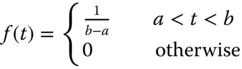
A random variable is defined as uniformly distributed over the interval of [a, b] when the probability of taking any value between a and b is equally likely. Let T be the random variable of the uniform distribution; the PDF is defined as
The CDF, denoted as F(t), is given by
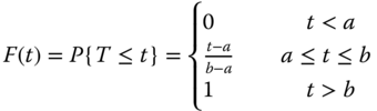
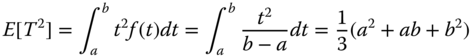
The mean and variance of T are given by

When a = 0 and b = 1, the PDF in Eq. 1.6.1 is called the standard uniform distribution, which is denoted as U[0, 1]. In Bayesian reliability inference, the standard uniform distribution is frequently used as a prior distribution for a component or system reliability estimate when the actual reliability is unknown, or is hard to deduce because of insufficient failures or testing time.
1.6.2 The Exponential Distribution
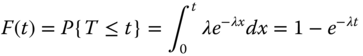
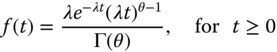
The random variable of the exponential distribution is continuous and non‐negative. Hence it is an ideal random variable to model the lifetime of products and system. If T is exponentially distributed, then the PDF is given as follows:
where λ is the distribution parameter and λ > 0. The CDF and reliability function are defined as
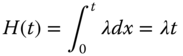
Both the hazard rate function and the cumulative hazard rate function are
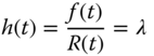
For exponential lifetime distribution, the hazard rate function is a constant, or vice versa. This observation leads to an important feature of exponential random variable, that is, memoryless property. Let s be the length of time (such as hours) that the system has survived. For a random variable T possessing the memoryless property, the following equality always holds:
The proof of the equality is given below:

It states the probability that the product will survive for s + t hours, given that it has survived s hours is the same as the initial probability that it survives for t hours. Finally, the mean and the variance of T are obtained and given as


1.6.3 The Weibull Distribution
The Weibull distribution perhaps is the most widely used continuous probabilistic model to analyze the time‐to‐failure behavior of components, systems, or equipment in a reliability community. A book dedicated to the Weibull model and its application was written by Murthy et al. (2003). Below we briefly review and Weibull distribution properties pertaining to lifetime modeling. A random variable T is said to follow a Weibull distribution if it possesses the following PDF:
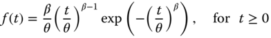
where θ and β are the scale and shape parameters, respectively. In general, θ > 0 and 0 < β < ∞. The CDF is given as

the Weibull reliability function is

and the hazard rate function is

The popularity of the Weibull distribution lies in its versatility of h(t). One can model a decreasing (0 < β < 1), constant (β = 1), or increasing hazard rate (β > 1) by simply changing the value of β. Figures 1.12–1.14 depict the hazard rate, PDF, and reliability function with different β. Since θ is a scale parameter, it is normalized at θ = 1 in these charts.

Figure 1.12The hazard rate of the Weibull function.

Figure 1.13Weibull probability density function.
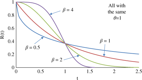
Figure 1.14 Weibull reliability function.
Finally, the mean and the variance of the Weibull random variable are given as follows:
1.6.4 The Normal Distribution
The normal distribution, also known as Gaussian distribution, perhaps is the most widely used continuous distribution model applied in engineering and science fields, including a reliability analysis. A random variable T is said to be normally distributed if the PDF exhibits the following form:
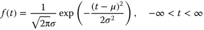
where μ and σ are the scale and the shape parameters, respectively. The normal density function has a bell‐shaped curve that is symmetric around μ. Figure 1.15 plots the normal PDF for {μ = 20, σ = 3}, {μ = 20, σ = 5}, and {μ = 35, σ = 5} for comparison purposes.

Figure 1.15Normal PDF under different means and variances.
The mean and the variance of T are equal to the parameters μ and σ2, respectively,
The reliability function is

where Φ(z) denotes the standard normal cumulative distribution with μ = 0 and σ = 1. Unlike the Weibull distribution, there is no closed‐form expression for Eq. 1.6.31. To estimate R(t) at given t, tables are created to list the possible cumulative value for Φ(z).
1.6.5 The Lognormal Distribution
The lognormal distribution is one of the most frequently used parametric distributions in analyzing reliability data of microelectronic devices in semiconductor manufacturing industry. The reason why semiconductor life data fit the lognormal distribution well is because the lognormal distribution is formed by the multiplicative effects of random variables. This type of multiplicative interactions is often encountered in many semiconductor failure mechanisms (Oates and Lin 2009; Filippi et al. 2010). A random variable T is said to follow a lognormal distribution when the transformed variable X = log(T) is normally distributed. The PDF for T is given by
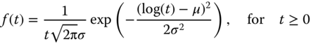
Two parameters μ and σ are required to define a lognormal distribution, where μ is called the scale parameter and σ is the shape parameter. Unlike the normal distribution where the mean and the standard deviation, respectively, equal the scale and shape parameter, the mean and the variance of the lognormal random variable are estimated by
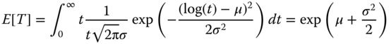

Figure 1.16 plots the lognormal distribution for σ = 0.25, 0.5, and 1 with common μ = 2. The lognormal PDF with a smaller σ tends to resemble the bell shape of a normal distribution.
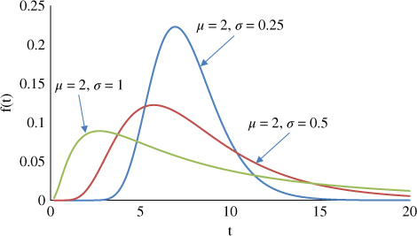
Figure 1.16Lognormal PDF plots.
1.6.6 The Gamma Distribution
The gamma distribution is often used to model the number of errors in multilevel Poisson regression models, because the combination of the Poisson distribution and a gamma distribution is a negative binomial distribution. In Bayesian reliability statistics, the gamma distribution is often chosen as a conjugate prior for the distribution parameter to be estimated. For instance, the gamma distribution is the conjugate prior for the exponential lifetime distribution. The PDF of a random variable T with the gamma distribution is given as
with

where λ and θ are the distribution parameters and both are positive values. Equation 1.6.37 is called the gamma function. If θ is a non‐negative integer, then Γ(θ) = (θ − 1)!. The mean and the variance of the Gamma random variable is (Ross 1998)
Figure 1.18 plots the gamma PDF with different pairs of λ and θ. Two types of PDF curves are available depending on the values of λ and θ. For 0 < θ ≤ 1, the PDF function declines monotonically with t. When θ > 1, the PDF resembles the bell‐shape type of curve. By varying the values of λ and θ, one can obtain various shapes of gamma PDF curves. Similar to the Weibull distribution, the gamma distribution is also capable of modeling a decreasing, constant, increasing failure rate corresponding to 0 < θ < 1, θ = 1, and θ > 1, respectively.

Figure 1.18Gamma PDF plots.
For a special case where θ are positive integers in Eq. 1.6.36, say θ = n = 1, 2, 3, …, the gamma distribution arises as the distribution of the amount of time one needs to wait until a total of n events has occurred. To prove that, let Tn denote the time at which the nth event occurs and note that Tn is less than or equal to t if and only if the number of events occurred by t is at least n; namely,
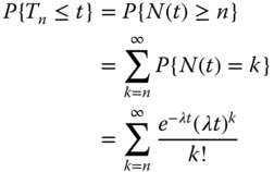
where the final identity follows, since the number of events in [0, t] has a Poisson distribution with parameter λt. Taking the derivative with respect to t in Eq. 1.6.40 yields the PDF of Tn as follows:
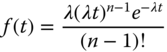
Hence Tn is a gamma distribution with parameters (λ, n). This distribution is often referred to as the n‐Erlang distribution, which is a special case of a gamma distribution with θ being positive integers. If θ = 1, the gamma distribution is reduced to an exponential distribution (also see Figure 1.18). Amari and Misra (1997) derived a closed‐form expression for distribution of the sum of exponential random variables, which is very useful for reliability analysis if a system is comprised of multiple components, each having a constant failure rate.
1.7 Bayesian Reliability Model
1.7.1 Concept of Bayesian Reliability Inference
Lifetime or failure models, as we discussed earlier, have one or more unknown distribution parameters. The classical statistical approach considers these parameters as fixed but unknown constants. They can be estimated using sample data taken randomly from the population. For instance, the value of parameter λ in the exponential PDF is assumed to be fixed and can be estimated. For an unknown parameter, a probabilistic statement represents the likelihood that the values calculated from a sample capture the underlying true parameter.
Unlike the classic statistical approach, Bayesian analysis treats the distribution or population parameters as random instead of being a fixed quantity. Historical data or subjective judgments can be used to determine a prior distribution for these parameters. The primary motivation to use Bayesian reliability methods is a desire to save on the test time and materials cost by leveraging the historical information of similar products or expert knowledge.
Figure 1.19 graphically shows a two‐step Bayesian inference process. First, we use historical data, or subjective information, to construct a prior distribution for these unknown parameters. This model represents our initial assessment about how likely various values of the unknown parameters are. We then combine the current or new data with the prior distribution to revise this initial assessment, deriving what is called the posterior distribution model for the distribution parameters. Parameter estimates are then calculated directly from the posterior distribution. In applying the Bayes formula, conjugate prior models are a natural option to represent the parametric prior distribution. In many applications it is uncommon that historical data are available or exist to validate a chosen prior model. In that case uniform distributions are often chosen and designated as the uninformative prior probability model for the parameters to be estimated.
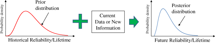
Figure 1.19Bayesian reliability inference process.
1.7.2 Bayes Formula
The Bayes formula is the mathematical tool that can combine prior knowledge with current data to produce a posterior distribution. Let E and F be two random events. The Bayes formula for discrete events is given as

and P{F} in the denominator is further expanded by using the “Law of Total Probability” as
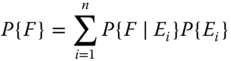
with the events Ei being mutually exclusive and exhausting all possibilities with ![]() .
.
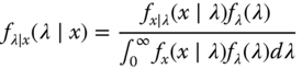
Next we present the Bayes formula for the continuous random variables. Let λ be the unknown distribution parameter to be estimated and x be the observed data. Assuming λ and x are continuous random variables, the Bayes formula in terms of PDF models takes the form as
where
- fλ(λ) = the prior distribution model for λ
- fλ|x(λ|x) = the posterior distribution for λ given that the current data x observed
- fx|λ(x|λ) = the likelihood function for observed data x with unknown parameter λ
When fλ(λ) and fλ|x(λ|x) both belong to the same distribution family, they are called conjugate distributions. Meanwhile fλ(λ) is the conjugate prior for fx|λ(x|λ). For example, the gamma distribution model is a conjugate prior for the hazard rate λ when failure times or repair times are sampled from an exponentially distributed population. In fact the gamma‐exponential conjugate pair is used widely in Bayesian reliability inference because the posterior distribution for λ is also a gamma distribution.
1.8 Markov Model and Poisson Process
1.8.1 Discrete Markov Model
Let Xt be the value of the system characteristic at time t. Since Xt is not known with certainty before time t, it can be viewed as a random variable. A discrete time stochastic process is simply a sequence of random variables X1, X2, …, where Xi is represents the value at different times.
A discrete‐time stochastic process, or random sequence, is called a Markov chain if, for i = 0, 1, 2, …, all states satisfy the following condition:
This equation essentially says that the probability distribution of the state at time t + 1 depends only on the state at time t and does not depend on its previous states when the chain passed through on the way to state it at time t.
Since the Markov chain is a stationary process, the states within the Markov chain are time‐invariant. Now Eq. 1.8.2 can be simplified as
where pij is the probability that given the system is in state i at time t, the system will be in state j at time t + 1. Hence pij is also called the “transition probability.” Given the Markov chain has n states, all the transition probability values can be represented as an n × n square matrix:

Note that summation of the entries in a row must be equal to one. That is,

Let π = [π1, π2, …, πn] be the steady‐state probability for state j for j = 1, 2, …, n. For an ergodic Markov chain, the steady‐state probability can be computed by (where “T” is for transpose):
where P is the transition matrix in Eq. 1.8.4, and “T” is for the matrix or vector transposition. The Markov model can be used to analyse the reliability of a multi‐state system of which the system reliability deteriorates over time, starting from the good state initially, transitioning to a degradation state, and finally entering the failure state.
1.8.2 Birth–Death Model
The birth–death model is a continuous‐time Markov chain, denoted as an M/M/1 queue, for which the system state at any time is a non‐negative integer. Most of the Markov chains with exponential arrival and exponential service time can be modeled by the birth–death process. Figure 1.20 shows the transition diagram of the M/M/1 queue.
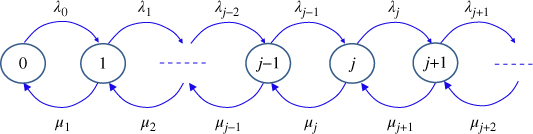
Figure 1.20Transition diagram for the birth–death queuing system.
In the transition diagram, λj for j = 0, 1, 2, … is called the birth rate and μj for j = 1, 2, 3, … is called the death rate. They are analogous to the transition probability in the discrete Markov chain. The steady‐state probability πj for state j can be solved using the flow balance equation. The following linear equation systems can be formulated:
The identity formula states that sum of all the steady‐state probabilities equals unity. That is,
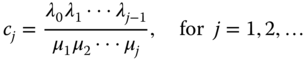
To solve this linear system, all πj (for j ≥ 1) can be recursively expressed as the function of π0 based on the above flow balance equations. The final results are given below:
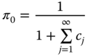
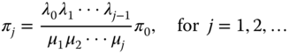
with
Quite often, we are interested in the time that a customer spends in the queue system including his/her waiting time, the processing time, as well as the number of customers in waiting or under service. They are defined in Table 1.3. We are now able to link these performance measures through the powerful law called Little's law, which states that
Table 1.3 Notation of queuing system.
| Notation | Interpretation |
| λ | Customer arrival rate (number of persons per unit time) |
| L | Average number of customers in the queuing system |
| Lq | Average number of customers waiting |
| Ls | Average number of customers being processed |
| W | Average time a customer spends in the queuing system |
| Wq | Average time a customer is waiting in the queue |
| Ws | Average time a customer spends with the server |
For any queue process, the following formulas always hold:

The birth–death queue model is perhaps the most basic queuing model. There are many different variations of queuing models, and readers are referred to the book by Winston (2004) on this topic.
1.8.3 Poisson Process
A Poisson process is a continuous‐time stochastic process that counts the number of events and the time epochs at which these events occur in a given time interval, say [0, t]. The interarrival time between two consecutive events has an exponential distribution with parameter λ, and all these interarrival times are assumed to be mutually independent. The process is named after the Poisson distribution introduced by the French mathematician Simeon D. Poisson (Poisson 1937). In reliability engineering, the Poisson process describes the time of events of equipment failures, demand stream of spare parts, and renewal of repairable systems. It has other applications in representing the time of events in telephone calls at a call center (Willkomm et al. 2009), tracking the requests on a web server (Arlitt and Williamson 1997), and many other punctual sequences where events take place independently among each other. Let N be the number of events occurred in [0, t]. The PDF for a Poisson process is

The expected value and the variance of X for the Poisson distribution is given by
References
- Amari, S.V. and Misra, R.B. (1997). Closed‐form expressions for distribution of sum of exponential random variables. IEEE Transactions on Reliability 46 (4): 519–522.
- Arlitt, M.F. and Williamson, C.L. (1997). Internet web servers: workload characterization and performance implications. IEEE/ACM Transactions on Networking 5 (5): 631–642.
- ASN, 2017, Aviation Safety Network, available at: https://aviation‐safety.net (accessed on May 30, 2017).
- Blischke, W.R. and Murthy, D.N.P. (2000). Reliability Modeling, Prediction, and Optimization. New York, NY: Wiley.
- Cai, Z., Sun, S., Si, S., and Yannou, B. (2011). Identifying product failure rate based on a conditional Bayesian network classifier. Expert Systems with Applications 38 (5): 5036–5043.
- Chowdhury, A.A. and Koval, D.O. (2009). Power Distribution System Reliability. Hoboken, NJ: Wiley and IEEE Press.
- Elsayed, E. (2012). Reliability Engineering, 2e. Hoboken, NJ: Wiley.
- Farrel, J. and Saloner, G. (1986). Installed base and compatibility: innovation, product preannouncements, and predation. The American Economic Review 76 (5): 940–955.
- Filippi, R.G., Wang, P.‐C., Brendler, A., and Lloyd, J.R. (2010). Implications of a threshold failure time and void nucleation on electromigration of copper interconnects. Journal of Applied Physics 107 (103709): 1–7. doi: 10.1063/1.3357161.
- Guikema, S.D. and Paté‐Cornell, M.E. (2004). Bayesian analysis of launch vehicle success rates. Journal of Spacecraft and Rockets 41 (1): 93–102.
- Gupta, R.C. and Bradley, D.M. (2003). Representing the mean residual life in terms of the failure rate,” . Mathematical and Computer Modelling 37 (12/13): 1271–1280.
- Jin, T. and Liao, H. (2009). Spare parts inventory control considering stochastic growth of an installed base. Computers and Industrial Engineering 56 (1): 452–460.
- Liao, H., P. Wang, T. Jin, S. Repaka, “Spare parts management considering new sales,” in Proceedings of Annual Reliability and Maintainability Symposium, 2008, pp. 502–507.
- Murthy, D.N.P., Xie, M., and Jiang, R. (2003). Weibull Models. Hobken, NJ: Wiley.
- Nachlas, J. (2016). Reliability Engineering: Probability Model and Maintenance Method, 2e. Boca Raton, FL: CRC Press.
- NIST, (2017), Engineering Statistics Handbook, Chapter 8, available at: http://www.itl.nist.gov/div898/handbook/apr/section1/apr125.htm (accessed on May 20, 2017).
- Oates, A.S. and Lin, M.H. (2009). Electromigration failure distributions of Cu/Low‐k dual‐damascene vias: impact of the critical current density and a new reliability extrapolation methodology. IEEE Transactions on Device and Materials Reliability 9 (2): 244–254.
- O'Connor, P.D.T. (2012). Practical Reliability Engineering, 4e. West Sussex, UK: Wiley.
- Poisson, S.D. (1937). Probabilité des Jugements en Matière Criminelle et en Matière Civile, Précédées des Règles Générales du Calcul des Probabilitiés, 206. Paris, France: Bachelier.
- Ross, S. (1998). A First Course in Probability, 5e. Upper Saddle River, NJ: Prentice Hall.
- Tse, K.‐K. (2014). Some applications of the Poisson process. Applied Mathematics 5 (19): 7.
- Wikepedia, (2017), “List of rail accidents in China,” available at: https://en.wikipedia.org/wiki/List_of_rail_accidents_in_China (accessed on May 30, 2017).
- Willkomm, D., Machiraju, S., Bolot, J., and Wolisz, A. (2009). Primary user behavior in cellular networks and implications for dynamic spectrum access. IEEE Communications Magazine 47 (3): 88–95.
- Winston, W.L. (2004). Operations Research: Application and Algorithm, 4e. Belmont, CA: Brooks/Cole.
Problems
The definition of the reliability is given in Eq. (1.2.1). What are the four conditions for this probability model?
- Problem 1.2 Problem Please state the definition of hazard rate and failure intensity rate. Explain their applications in reliability analysis in the context of repairable and non‐reparable systems/components. Is the bathtub curve applicable to both non‐repairable and repairable systems?
- Problem 1.3 Problem Please derive the analytical expressions for H(t), R(t), and f(t) given the following hazard rate functions: (1) h(t) = 3; (2) h(t) = 3 + 2t; and (3) h(t) = 3t0.5.
- Problem 1.4 Problem Please plot the h(t), H(t), R(t), and f(t) in three cases in Problem 1.3, respectively.
- Problem 1.5 Problem The power law function λ(t) = αβtβ − 1 has been widely used to model the failure intensity rate for a decreasing, constant, or increasing trend. Note that α and β are positive parameters. If 0 < β < 1, it represents a decreasing failure intensity rate. If β = 1, this is a constant failure intensity rate. If β > 1, it represents an increasing failure intensity rate. Please draw the power law function with {α = 30, β = 0.5}, {α = 10, β = 1}, {α = 2, β = 1.5}, and {α = 0.5, β = 2}, respectively.
- Problem 1.6 Problem If the failure intensity rate observes the power law function λ(t) =αβtβ − 1, estimate the cumulative number of failures in the intervals of [0, t = 10] and [t = 10, t = 20], respectively, assuming the following cases: (1) {α = 30, β = 0.5}; (2) {α = 10, β = 1}; and (3){α = 0.5, β = 2}.
- Problem 1.7 Problem After introducing nine identical new products to the market, the service engineer is able to collect the time‐to‐failure between the installation time and the failure times: 11, 21, 34, 36, 50, 60, 66, 72, 77, 111, 115, 140, 157, 209, 296, and 397 days. Do the following: (1) estimate the mean‐time‐to‐failure; (2) estimate the standard deviation of the product lifetime; (3) estimate the cumulative distribution of the product lifetime; (4) does the lifetime follows the exponential distribution? (Hint: use the statistic software to perform a probability fit); (5) based on the fitted lifetime distribution, derive the hazard rate function; (6) derive the reliability function.
- Problem 1.8 Problem A repairable system comprised of two different types of components connected in series. The system fails if one of the components is malfunctioning. Upon failure, the faulty component is removed and replaced with a good one and the system is recovered to the operational state. The failure arrival time of two types of components over 16 months are recorded: for component type one: 9, 25, 79, 195, 280, 311, 378, 452, and 455 days and for component type two: 16, 88, 147, 196, 242, 280, 349, 400, and 443 days. Estimate: (1) the hazard rate of each component type; (2) the failure intensity rate or ROCOF of the system; (3) does the component hazard rate function possess a decreasing, constant, or increasing trend? How about the ROCOF of the system?, and (4) if the replacement of a faulty component takes 10 hours on average, estimate the steady‐state system availability.
- Problem 1.9 Problem Estimate the cumulative hazard rate, reliability, PDF, and CDF given the hazard rate function: (1) h(t) = 10; (2) h(t) = 5t; (3) h(t) = 2 + 3t; (4) h(t) = 4t2; and (5) h(t) = 10t with 0 < t < 10).
- Problem 1.10 Problem A bin of four electronic components is known to contain two defective units. The components are to be tested one at a time, in random order, until both defectives are discovered. Calculate the expected number of tests that are made.
- Problem 1.11 Problem A machine could break down for two reasons: aging of the machine or inappropriate use by the operator. To check the first possibility, it would cost c1. The cost of repairing a breakdown machine because of aging is r1 dollars. Similarly, there are costs of c2 and r2 associated with breakdown or operator errors. Let p and 1 − p represent, respectively, the probability of breakdown due to machine aging and inappropriate use. Should the aging check be carried out first or should the check for impropriate use be done first? In other words, determine the relationship between p, c1, c2, r1, and r2 in two different checking sequences such that the total cost is minimized.
- Problem 1.12 Problem A four‐engine plane can fly reliably when only two of its engines are working. Similarly, a two‐engine plane can fly if only one of them is working. Suppose that the airplane engine fails with probability 1 − p independently from engine to engine. For what value of p is a four‐engine plane preferable to a two‐engine plane?
- Problem 1.13 Problem Suppose that 5% of the microdevices produced by a semiconductor manufacturer are defective. If we purchase 100 such devices, will the number of defective devices we receive be a binomial random variable? What is the probability that at least 10 units we received are defective?
- Problem 1.14 Problem The expected number of typographical errors on a page of a book is 0.1 error/page. What is the probability that the next page you read contains (1) no error; (2) two or more typographical errors?
- Problem 1.15 Problem For a Poisson random variable N with parameter λ, show that E[N] = λ and Var(N) = λ.
- Problem 1.16 Problem Let X be a binomial random variable with parameter (n, p). What value of p maximizes P{X = k} where the random variable is observed to equal k with 0 ≤ k ≤ n. If we assume n is known, then we estimate p by choosing the value for p that maximizes P{X = k}. This is known as the maximum likelihood estimation.
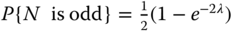
- Problem 1.17 Problem Let N be a Poisson random variable with parameter λ. Show that the following property is valid (Hint: use the relationship between the Poisson and binomial random variable):
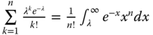
- Problem 1.18 Problem Show that
- Problem 1.19 Problem Prove that the variance of the Bernoulli random variable is Var(X) = p(1 − p).
- Problem 1.20 Problem The probability of an item failing is p = 0.001. What is the probability of 3 failing out of the population of n = 170? Solve the problem using the binomial distribution and Poisson distribution, respectively.
- Problem 1.21 Problem WTs are repairable systems. Reliability plays an important role as equipment maintenance and repair are costly. WT manufacturer A claims that MTBR of his product is exponentially distributed with 10 000 hours. Manufacturer B claims that MTBR of his product follows the Weibull distribution with θ = 11 000 hours, and β = 2.5. Assuming the repair and replacement cost of each failure are the same for two WT systems, decide which manufacturer is considered as the preferred supplier?
- Problem 1.22 Problem Based on the statement of the previous problem, the MTTR for WT of manufacturer A is five days and for B it is four days. From the equipment availability perspective, which manufacturer is more competitive in terms of sustaining the uptime of the equipment?
- Problem 1.23 Problem The main landing gear leg of a large commercial airplane usually contains six tires. Experience shows that a tire bursts on average on 1 out of 2000 landings. Assuming that a tire burst occurs independently of other tires and a safe landing is made as long as no more than two tires burst, what is the probability of an unsafe landing?
- Problem 1.24 Problem A product with an exponential lifetime distribution has a hazard rate of h(t) = λ. Let T be the random lifetime. Prove:
- Compute E[T] = 1/λ.
- Compute E[T2] = 2/λ2.
- Estimate E[T] and E[T2] given (1) λ = 1; (2) λ = 0.5; and (3) λ = 3, respectively.
- Problem 1.25 Problem A product's lifetime is exponentially distributed with parameter λ = 0.001 failures/hour. Do the following: (1) estimate the mean lifetime for this product; (2) draw the PDF; (3) draw the CDF function; (4) draw the reliability function; and (5) draw the failure rate function. (Note: Draw all of the curves on a separate chart.)
- Problem 1.26 Problem Suppose that the number of miles that an EV can run before its battery wears out is exponentially distributed with an average distance of 100 000 miles. If a car manufacturer decides to install this type of battery to power the EV, what percentage of the cars will fail at the end of 50 000 and 100 000 miles, respectively?
- Problem 1.27 Problem Based on the previous problem, the car manufacturer is not satisfied with the lifetime of the battery that is supplied by its subcontractor. The manufacturer wants the car to operate after running 100 000 miles with a probability of 80%. What should the minimum mean lifetime of the battery be in order to meet the new requirement?
- Problem 1.28 Problem Given the Weibull PDF, f(t) = αβ(αt)β − 1 exp(−(αt)β), where α > 0 and β > 0 are the scale and shape parameters, respectively. Plot the PDF, CDF, reliability, and hazard rate under different values of β = 0.5, 1, 1.5, 2, and 3, respectively. In all cases, α = 2.
- Problem 1.29 Problem (Normal) Let T be a normal random variable with N(μ, σ2). Prove that E[T] = μ and E[T2] = μ2 + σ2.
- Problem 1.30 Problem (Lognormal) Let T be a lognormal random variable with scale parameter μ and shape parameter σ. Prove that

(Hint: Using the normal moment generating function to find the mean and variance of T.)
- Problem 1.31 Problem (Gamma) Let T be a gamma random variable with parameters λ and θ. Do the following:
- (1)
Prove that
 and
and 
- (2) For λ = 1 and θ = 3, find the reliability R(T > 2).
- (3) For λ = 1 and θ = 3.5, find the reliability R(T > 2).
- (1)
Prove that
- Problem 1.32 Problem For exponentially distributed lifetime T, show that
P{T < t + s ∣ T > s} = P{T < t}, for t > 0 and s > 0
- Problem 1.33 Problem Suppose that p(x, y), the joint probability mass function of X and Y, is given by
p(0, 0) = 0.4, p(0, 1) = 0.2, p(1, 0) = 0.1, and p(1, 1) = 0.3. Calculate the conditional probability mass function of X, given that Y = 0 and Y = 1, respectively.
- Problem 1.34 Problem The joint density of X and Y is given by

Find fX ∣ Y(x ∣ y), that is, the conditional density of X, given that Y = y, where 0 < y < 1.
- Problem 1.35 Problem For the birth–death M/M/1/∞ model, assume λj = λ for all j = 0, 1, 2, and μj = μ for all j = 1, 2, 3, …. Define ρ = λ/μ. Show the following results:
(1) π0 = 1 − ρ; (2) L = ρ/(1 − ρ); (3) Ls = ρ.