
2
Reliability Estimation with Uncertainty
2.1 Introduction
This chapter introduces the reliability block diagram and presents reliability estimation methods for a variety of system structures, including series, parallel, mixed series‐and‐parallel, k‐out‐of‐n redundancy, and networks. The focus is on modeling and analysis of the uncertainty of component reliability estimates and its impact on the system reliability performance. Particularly, we propose block decomposition methods to calculate the variance of a system reliability estimate based on the moments of a component reliability estimate. Reducing reliability estimation uncertainty is of importance in terms of designing and operating risk‐averse systems in private and public sectors, including manufacturing, healthcare, transportation, energy, supply chains, and defense industries, where failures often lead to costly downtime or even human casualty. System reliability confidence intervals (CIs) are further derived under binomial, normal, and lognormal distributions. We also extend the binary reliability models to multistate systems. This chapter is concluded with the discussion of reliability importance measures.
2.2 Reliability Block Diagram
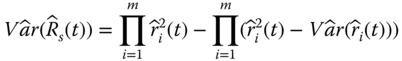
A reliability block diagram (RBD) is a graphical representation to capture the functional or operational interdependency of different components in a system. Each block represents a component or subsystem that possesses its own failure rate or reliability feature. For instance, if blocks are connected in series, any failure along a series path causes the whole system to fail. Parallel configuration of blocks means that the system is operational as long as one of the parallel paths is still good. Regardless of physical structure, there exist four basic types of functional relationships between a system and its components. These are series, parallel, k‐out‐of‐n redundancy, and network systems. Figure 2.1 shows the reliability diagrams of these systems.

Figure 2.1Reliability block diagrams of basic system structures.
The configuration of a complex system is often the mix of two or more of these basic block diagrams. For example, reliable supply of electricity requires the generators, the transmission/distribution lines and the transformers all to work properly. At the operational level, these components are connected and functioning in series stretching dozens or hundreds kilometers. Figure 2.2 depicts the series connection between power generation, transmission, distribution, and consumption.

Figure 2.2Series reliability block diagram of the electric power system.
Meanwhile, the generation pool consists of multiple power units and can be treated as a k‐out‐of‐n redundant system. In a substation where many transformers work as a parallel system to escalate the voltage or reduce the voltage to facilitate the power delivery. Transmission lines are often interconnected to form a meshed network and the distribution system is created as a radial network with multiple feeders connected to one single substation. Figure 2.3 depicts the structural view of different types of reliability block diagrams across power generation, transmission, distribution, and consumption.
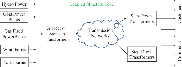
Figure 2.3Reliability block diagram of the power system at the structure level.
2.3 Series Systems
2.3.1 Reliability of Series System
A series system is comprised of multiple components interconnected in a sequential manner either physically or functionally. Typical examples of series systems include low‐voltage power distribution circuits, oil pipelines, automobile assembly lines, computers, and air‐conditioning systems. For a series system, failure of any component leads to the malfunction of the entire system. For example, a modern wind turbine can be treated as a series system comprised of multiple electromechanical components, including blades, main bearing/shaft, gearbox, generator, direct current (DC)–alternating current (AC) converters, and auxiliary parts. Failure of any component such as a blade or a gearbox usually brings the turbine to a down state, despite other components still remaining functional.
A series system could also be the case where the functionality of the entire system is treated as multiple components connected in series. However, components may not be physically configured in series format. For example, an automobile typically has four tires that are not formed in a linear configuration, yet they are treated as a series system in reliability analysis. This is because all tires must operate appropriately in order to ensure the normal driving function.
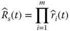
A reliability block diagram of a series system comprised of m components is shown in Figure 2.4. Note that ri(t) is the reliability of the ith component for i = 1, 2, …, m. Let Rs(t) be the reliability of the series system; then

where Ti is the lifetime of component i and ri(t) is the associated reliability at time t. Equation 2.3.1 is derived based on the assumption that all components fail independently.

Figure 2.4A series system comprised of m components.
2.3.2 Mean and Variance of Reliability Estimate
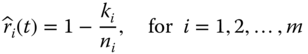
In reality the true component reliability ri(t) is not known and its estimate, denoted as ![]() , is often used to infer the true value. Then the reliability estimate of the series system, denoted as
, is often used to infer the true value. Then the reliability estimate of the series system, denoted as ![]() , becomes
, becomes
Reliability estimates are often derived from the assumption that the component or the system lifetime distribution can be represented with a parametric model, such as exponential and Weibull distributions. This assumption could be misleading if the estimation involves considerable amounts of uncertainty (Borgonov 2007). This situation usually happens when sufficient field or experimental data are not available to infer the underlying lifetime distribution. To design a risk‐averse system, the uncertainty of component reliability estimates needs to be explicitly analyzed and appropriately incorporated into the system reliability estimation model.
The uncertainty of the component reliability estimate can be quantified by its moments, such as mean and variance. Figure 2.5 depicts the probability density functions of ![]() and
and ![]() , corresponding to components 1 and 2, respectively. For a risk‐neutral system design, component 1 is better than component 2 because
, corresponding to components 1 and 2, respectively. For a risk‐neutral system design, component 1 is better than component 2 because ![]() >
> ![]() . However, if a risk‐averse design is preferred, component 2 tends to be better than component 1 because its variance
. However, if a risk‐averse design is preferred, component 2 tends to be better than component 1 because its variance ![]() is much smaller.
is much smaller.

Figure 2.5Distributions of component reliability estimates.
Different approaches are available to determine the reliability estimate and the associated variance. One common approach is to treat the number of failures as a binomial random variable in a given period of time. For instance, considering a system consisted of m different components, ni units are allocated for reliability testing for component i for i = 1, 2, …, m. Each unit is tested for t hours and ki failures are observed during [0, t]. The status (survival or failure) of each testing unit can be treated as an independent Bernoulli trial with parameter ri(t). That is, the number of survivals Xi is a random variable following the binomial distribution B(ni, ri(t)). An unbiased estimate of ![]() and the associated variance can be estimated by (Coit 1997)
and the associated variance can be estimated by (Coit 1997)

In statistics an estimate is said to be unbiased if the mean of the sampling distribution of that statistic is equal to the estimating parameter. To show that Eq. 2.3.5 is an unbiased estimate for ![]() , we compute the expectation of the variance estimate as follows:
, we compute the expectation of the variance estimate as follows:
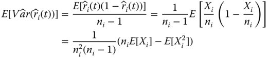
Recalling that Xi, the number of components i surviving in [0, t], follows the binomial distribution with B(ni, ri). From Eqs. (1.5.5) and (1.5.6), the first two moments of Xi are given as
By substituting Eqs. 2.3.7 and 2.3.8 into Eq. 2.3.6, we have

This result is equivalent to Eq. (1.5.7) divided by ni2. This completes the proof that Eq. 2.3.5 is the unbiased estimate of ![]() .
.
Given the reliability block diagram, we can further compute the mean and variance of the system reliability estimate based on the moments of component reliability estimates. Let ![]() be the reliability estimate of a series system in Eq. 2.3.3. The mean and the variance of
be the reliability estimate of a series system in Eq. 2.3.3. The mean and the variance of ![]() can be computed as follows (Jin and Coit 2008):
can be computed as follows (Jin and Coit 2008):
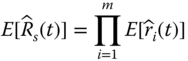
Statistically, Eq. 2.3.11 measures the proportion of the unconditional variance of ![]() that can be attributed to the mean and the variance of
that can be attributed to the mean and the variance of ![]() for i = 1, 2, …, m. Both
for i = 1, 2, …, m. Both ![]() and
and ![]() can assist the design engineers in identifying the components that have the largest contribution to the system reliability variability. Thus remedies or proactive measures can be taken to mitigate the reliability risks by adopting more reliable or less uncertain components for system configuration.
can assist the design engineers in identifying the components that have the largest contribution to the system reliability variability. Thus remedies or proactive measures can be taken to mitigate the reliability risks by adopting more reliable or less uncertain components for system configuration.
2.4 Parallel Systems
2.4.1 Reliability of Parallel Systems
A parallel system is one in which the proper operation of any one component or subsystem implies the functionality of the whole system. Typical examples of parallel systems include the multipump gas station, aircraft with dual engines, multilane highway, and distributed computing, among many others. Figure 2.6 shows the reliability block diagram of a parallel system that consists of m components, where ri(t) is the reliability of the ith component for i = 1, 2, …, m.
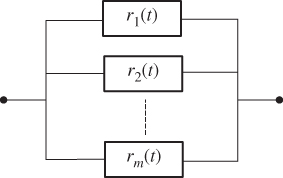
Figure 2.6Reliability diagram for a parallel system.
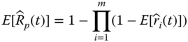
A main advantage of parallel configuration is that the system can achieve fault‐tolerant operation using redundant units even if the reliability of individual components is not high. For instance, an airplane powered with two engines is able to fly even if one of the engines fails. The reliability for a parallel system, denoted as Rp(t), can be estimated using
For instance, a parallel system consists of three components with r1 = 0.5, r2 = 0.6, and r3 = 0.7, respectively. The system reliability becomes Rp = 1 − (1 − 0.5) (1 − 0.6) (1 − 0.7) = 0.94. This example shows that high system reliability can be realized through the parallel configuration of low or medium reliability components.
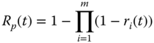
2.4.2 Mean and Variance of Reliability Estimate
Let ![]() be the estimate of the parallel system reliability and
be the estimate of the parallel system reliability and ![]() be the reliability estimate of component i for i = 1, 2, …, m. Assuming component reliability, estimates are statistically independent. Based on Eq. 2.4.1, the mean and variance of
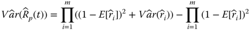
be the reliability estimate of component i for i = 1, 2, …, m. Assuming component reliability, estimates are statistically independent. Based on Eq. 2.4.1, the mean and variance of ![]() can be estimated as follows (Jin and Coit 2008):
can be estimated as follows (Jin and Coit 2008):
It is worth mentioning that Eqs. 2.4.2 and 2.4.3 are unbiased estimates for ![]() and
and ![]() , respectively. This is left as an exercise for the readers.
, respectively. This is left as an exercise for the readers.
2.5 Mixed Series and Parallel Systems
The systems discussed so far are pure series or pure parallel structures. There are many systems of which the components are configured in a mix of series and parallel modes. Generally these mixed structures can be classified into three categories: (i) series–parallel system, (ii) parallel–series system, and (iii) hybrid series and parallel system. This section presents the reliability estimation models for mixed configurations.
2.5.1 Series–Parallel System
A series–parallel system can be treated as a two‐level hierarchical structure. At the system level multiple subsystems are connected in series. At the subsystem level, components are configured in a parallel structure. Figure 2.7 shows a series–parallel system that is comprised of three subsystems, and each subsystem itself consists of two or three components in parallel.
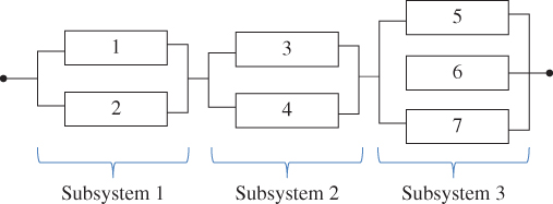
Figure 2.7A series–parallel system.
Let s be the number of subsystems and mj be the number of components within subsystem j for j = 1, 2, …, s. For instance, the series–parallel system in Figure 2.7 has s = 3, m1 = 2, m2 = 2, and m3 = 3. The reliability estimate of a series–parallel system, denoted as ![]() , can be estimated by
, can be estimated by

where ![]() is the reliability estimate of subsystem j and
is the reliability estimate of subsystem j and ![]() is the reliability estimate of component i for i = 1, 2, …, mj in subsystem j. Equation 2.5.1 shows that reliability estimation of a series–parallel system can be performed in two steps. In step one, we calculate the reliability of each subsystem based on parallel system reliability models in Eqs. 2.4.1 or 2.4.2. In step two, we multiply all the subsystem reliability models and obtain the whole system reliability using Eqs. 2.3.3 or 2.3.10. The mean of
is the reliability estimate of component i for i = 1, 2, …, mj in subsystem j. Equation 2.5.1 shows that reliability estimation of a series–parallel system can be performed in two steps. In step one, we calculate the reliability of each subsystem based on parallel system reliability models in Eqs. 2.4.1 or 2.4.2. In step two, we multiply all the subsystem reliability models and obtain the whole system reliability using Eqs. 2.3.3 or 2.3.10. The mean of ![]() , denoted as
, denoted as ![]() , can be obtained by substituting
, can be obtained by substituting ![]() with
with ![]() in Eq. 2.5.1 for all i and j. That is,
in Eq. 2.5.1 for all i and j. That is,
Let ![]() be the variance estimate of
be the variance estimate of ![]() . To obtain an unbiased estimate of
. To obtain an unbiased estimate of ![]() , Jin and Coit (2008) proposed a block decomposition method to propagate the variance of
, Jin and Coit (2008) proposed a block decomposition method to propagate the variance of ![]() from the component level to the system level. Without providing the detailed derivation, the unbiased estimate for
from the component level to the system level. Without providing the detailed derivation, the unbiased estimate for ![]() can be expressed as
can be expressed as
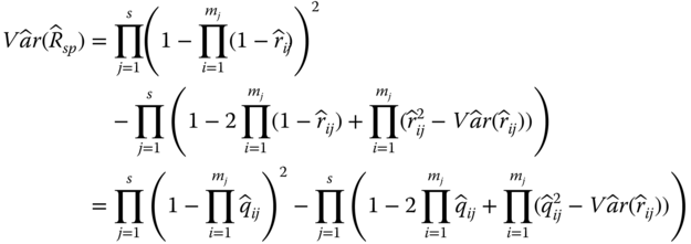
where ![]() is the unreliability estimate for component j in subsystem i, and
is the unreliability estimate for component j in subsystem i, and ![]() = 1 −
= 1 − ![]() . Based on Goodman's (1960) results, Ramirez‐Marquez and Jiang (2006) developed a recursive method to compute
. Based on Goodman's (1960) results, Ramirez‐Marquez and Jiang (2006) developed a recursive method to compute ![]() , which yields the same result as the block decomposition in Equation 2.5.3. The idea is to sequentially reduce one component each time the series or parallel decomposition is applied.
, which yields the same result as the block decomposition in Equation 2.5.3. The idea is to sequentially reduce one component each time the series or parallel decomposition is applied.
2.5.2 Parallel–Series System
For a parallel–series configuration, the system can be treated as an architecture with multiple subsystems configured in parallel. At the subsystem level, each subsystem is comprised of multiple components in series. Figure 2.8 shows a typical parallel–series system of which three subsystems 1, 2, and 3 are placed in parallel. Each subsystem is formed by two or three components connected in series. For instance, Subsystem 2 is formed by components 3, 4, and 5 in series.

Figure 2.8A parallel–series system.
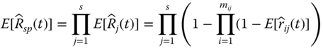
Let s be the number of subsystems and mj be the number of components in subsystem j for j = 1, 2, …, s. The reliability of the parallel–series system is given as
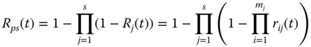
where Rj(t) is the reliability of subsystem j and rij(t) is the reliability of component i in subsystem j. Let ![]() be the estimate of Rps(t). To obtain the mean of
be the estimate of Rps(t). To obtain the mean of ![]() , we substitute rij(t) with its mean value
, we substitute rij(t) with its mean value ![]() in Eq. 2.5.4; that is,
in Eq. 2.5.4; that is,

Similarly, the estimate of ![]() is given as follows:
is given as follows:
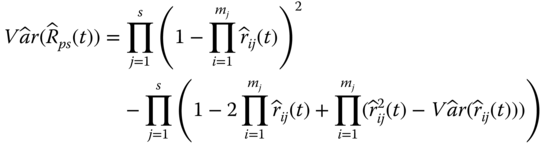
Both Eqs. 2.5.5 and 2.5.6 are the unbiased estimates for ![]() and
and ![]() , respectively. Again, we leave this as exercises for the readers.
, respectively. Again, we leave this as exercises for the readers.
2.5.3 Mixed Series–Parallel System
A mixed series–parallel system can be treated as a hierarchical structure that is embedded with series–parallel and/or parallel–parallel subsystems at different layers. Figure 2.9 shows a typical mixed series–parallel system comprised of four subsystems with a total of seven components. Subsystems 1 and 2 are pure parallel systems. Subsystem 3 is a series–parallel structure with component 4 and subsystem 2 in series. Subsystem 4 is equivalent to a parallel–series structure where component 7 is in parallel with subsystem 3.

Figure 2.9A mixed series–parallel system with seven components.
Given the reliability or the lifetime data at component levels, different methods such as series and parallel reduction can be applied to calculate the reliability of the mixed series–parallel system. Let ![]() be the reliability estimate of a mixed series–parallel system. A procedure for estimating
be the reliability estimate of a mixed series–parallel system. A procedure for estimating ![]() and
and ![]() for any systems that can be decomposed into series, parallel, or series–parallel structures are given as follows:
for any systems that can be decomposed into series, parallel, or series–parallel structures are given as follows:
- Step 1: Identify the reliability blocks (i.e. subsystems) based on series and parallel decomposition rules.
- Step 2: Begin with the most embedded subsystem. If it is a series configuration, compute the mean and the variance of the subsystem reliability estimate using Eqs. 2.3.10 and 2.3.11. If it is parallel, compute the mean and the variance of the subsystem reliability estimate using Eqs. 2.4.2 and 2.4.3.
- Step 3: Move to the upper level subsystem and apply series and parallel reduction recursively as in Step 2 until
 and
and  are obtained.
2.6 Systems with k‐out‐of‐n:G Redundancy
2.6.1 Reliability for Hot‐Standby Redundant Systems
A k‐out‐of‐n:G system, or simply called k‐out‐of‐n system, is the one in which the proper function of any k components (note that k ≤ n) or larger in the system implies the proper system function. A k‐out‐of‐n:G system is equivalent to an (n − k + 1)‐out‐of‐n:F system, where the system fails if n − k + 1 components are malfunctioning. To guarantee reliability and safety, wide‐body passenger aircraft such as Boeing 747 and Airbus 380 are powered with 2‐out‐4 engine systems. The plane can fly reliably as long as two engines are working. In the power industry the electric grid is required to meet the criterion of N – 1 fault tolerance, meaning the utility company is still able to meet the demand at the loss or failure of the largest generating unit.
Three types of k‐out‐of‐n systems are generally used in practical applications: hot standby, warm standby, and cold standby (Elsayed 2012). In hot standby mode, all n components are in operating mode, and the load is shared among themselves. For instance, the engine cluster in Boeing 747 belongs to the 2‐out‐4 hot standby redundancy as four engines simultaneously generate thrust during the flight. In warm standby, only k components undertake the load. The other n – k components, though in online mode, do not share the load. A redundancy array of independent disks (RAID) in the data center and the dual power distribution lines (primary and secondary) are typical examples of warm standby systems. Cold standby differs from hot standby and warm standby in that all of the redundant components are in off‐line mode. They need to be powered up and switched to the operating mode upon request. A good example of a cold standby system is the back‐up power generator on a university campus. For a repairable system, the inventory spare parts can be treated as the cold standby unit. If the field system fails, the faulty unit can be replaced with the spare part, and the system can return to the working state in a timely manner.
Let r(t) be the component reliability in the k‐out‐of‐n:G system in a hot standby mode. Assume all components are identical. The reliability of the redundant system, denoted as Rs(t), can be estimated by

It is worth mentioning that series and parallel systems are special cases of k‐out‐of‐n redundant systems. If k = n, Eq. 2.6.1 reduces to the series system reliability model in Eq. 2.3.3. If k = 1, Eq. 2.6.1 is equivalent to the parallel system reliability model in Eq. 2.4.1.
For a redundant system with warm standby components, Amari et al. (2012) derived a state‐space approach to reliability characterization for a k‐out‐of‐n warm standby system with identical components subject to exponential failure. In addition, they provide closed‐form expressions for the hazard rate, probability density function, and mean residual life function. Wu et al. (2017) developed a new modeling approach for availability evaluation of a k‐out‐of‐n:G warm standby redundancy system with repair. They showed that the performance evaluation process algebra turns out to be an efficient way to deal with the availability evaluation of systems with different groups of repairable components.
2.6.2 Application to Data Storage Systems
A redundant array of independent disks (RAID) is a data storage virtualization technology. It combines multiple disk drives to form a single logical unit for the purposes of data redundancy, parallel throughput, and information retrieval in large data centers. Figure 2.13 depicts the configuration of a RAID‐5 system with four disks connected in parallel. It employs one redundant disk to achieve fault tolerance that allows up to one disk failure. For example, a data file “A” is split into multiple segments A1, A2, and A3, each stored on Disks 1, 2, and 3, respectively. Disk 4 is used to store the parity codes of file “A”, denoted as PA (parity array). If one block of data fails to be retrieved from any one of Disks 1, 2, and 3, the parity codes in Disk 4 are used to reconstruct the damaged data sector by performing the reverse Boolean operation. During the reconstruction process, the bad sector of the data disk is mapped out. After the system rebuilds the damaged sector using the data from remaining good disks, the reconstructed data are saved in a good, yet unused, sector on the same disk. This self‐recovery process is called media repair or data restoration. Therefore, all stored data in the RAID‐5 system can be retrieved as long as three disks are functioning. Hence, a RAID‐5 system can be treated as a 3‐out‐of‐4 hot standby redundant system.

Figure 2.13A RAID‐5 system and its reliability block diagram.
The working principle of RAID‐6 is similar to RAID‐5 except that it has five disk drives and two of them are used as redundant disks for data recovery. Thus RAID‐6 can be treated as a 3‐out‐of‐5 hot standby redundant system.
2.7 Network Systems
2.7.1 Edge Decomposition
There are lots of applications where network architecture is required, such as highway transportation, power transmission, telecommunications, Internet, blood vessels of human beings, and integrated circuits. A network consists of a set of edges and nodes, and any node is connected by at least one edge. Figure 2.15 shows a five‐component bridge network, while most real‐world networks are far more complicated with dozens or even hundreds of thousands of components that are interconnected. Network reliability analysis deals with determining the reliability measures required for stochastic edge or node failures. Typical measures include the two‐terminal, the k‐terminal, and the all‐terminal reliability models. Most network reliability analysis problems are as hard as the NP‐complete problems (Ball 1986), namely, the computational time grows exponentially with the size of the network.

Figure 2.15A simple bridge network with five components.
In this section, we first present the edge decomposition method as it provides the exact solution to the two‐terminal network reliability estimation. Then we introduce two approximation methods: minimum path and minimum cut. The minimum path always results in the lower bound of the network reliability while the minimum cuts yield the upper bound of the network reliability estimation (Colbourn 1987). Finally, we discuss a linear‐quadratic minim cut model to estimate the mean and the variance of the two‐terminal network reliability estimate.

Figure 2.16A series–parallel system conditioned on a function of component 3.
The idea of edge decomposition is to sequentially reduce the network to a set of series and/or parallel systems by recursively applying conditional probability theory (Shier 1991). We use the bridge network in Figure 2.15 to illustrate the decomposition procedure. Without loss of generality, we start with component 3. Two scenarios need to be considered: component 3 is functioning or malfunctioning.
- Step 1: If component 3 is functioning, the bridge network can be transformed into a series–parallel system, shown in Figure 2.16.
The reliability of this decomposed series–parallel system, denoted as Rs1(t), can be readily obtained as follows:
2.7.1
- Step 2: If component 3 is malfunctioning, the bridge network is transformed into the following mixed series and parallel system.
The reliability of the decomposed system in Figure 2.17, denoted as Rs2(t), is given as follows:
where q3 is the unreliability of component 3 and q3 = 1 − r3. Finally, the reliability of the original network is obtained by aggregating Rs1(t) and Rs2(t). That is,
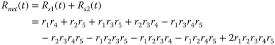

Figure 2.17A mixed series and parallel system conditioned on the failure of component 3.
Though the principle of edge decomposition is straightforward, the number of substructures resulted from the decomposition often grow exponentially with the size of the network. Next we introduce minimum cut and minimum path approaches that can handle large‐size networks more efficiently.
2.7.2 Minimum Cut Set
A cut vector, y, is a set of component status for which the corresponding system reliability becomes zero provided all these components fail. For example, in Figure 2.15 the component set y = {1, 2, 3} is a cut vector because failures of all these components render the network down. Other vectors such as {1, 3, 4, 5} and {2, 3, 4, 5} are also cut vectors.
A minimum cut vector, x, is a cut vector for which any vector y > x leads to non‐operation of the system. For example, component set x = {1, 2} is a minimum cut vector. If these components are not functional, the network is down. However, y = {1, 2, 3} is a cut vector, but not the minimum cut. This is because set {1, 2} is sufficient to bring the network down, and component 3 is not needed. Other vectors such as {4, 5}, {1, 3, 5}, and {2, 3, 4} are also minimum cuts. Given all these minimum cut sets, the bridge network can be transformed into the series–parallel system shown in Figure 2.18, where each cut set forms a parallel subsystem. Now the block decomposition can be applied to calculate the reliability of this series–parallel system. The resulting approximation is the upper bound of the true network reliability.

Figure 2.18The network with its equivalent series–parallel system.
We summarize the minimum cut set method for network reliability approximation in three steps:
- Step 1: Find all the minimum cut sets of the network and transform the network into a series–parallel system based on the minimum cut sets.
- Step 2: Compute the subsystem reliability of individual minimum cut sets based on a parallel system reliability estimate in Eq. 2.4.1.
- Step 3: Obtain the network reliability using the series system reliability estimate in Eq. 2.3.3.
2.7.3 Minimum Path Set
A path vector, y, is a component status vector for which the corresponding system reliability is assured provided all these components are operational. For example, component set y = {1, 2, 3, 5} is a path vector. Namely, the network is functional if all these components are working. Other vectors such as {1, 3, 4, 5} and {2, 3, 4, 5} are also path vectors.
A minimum path vector, x, is a path vector for which any vector x < y has a corresponding zero system reliability. For example, component set x = {1, 4} is a minimum path vector. If these components are working, the network is operational. If we remove any component from set x, the system is not always functional regardless of the reliability of remaining components. Set y = {1, 3, 4} is a path set, but not a minimum path set. The reason is if component 3 is malfunctioning, the path formed by {1, 4} still ensures the reliable connection between the source and the terminal nodes. Other vectors such as {1, 5}, {1, 3, 5}, and {2, 3, 4} are also minimum path vectors. Based on the minimum path sets, the bridge network can be transformed into a parallel–series system, as shown in Figure 2.19.
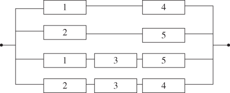
Figure 2.19Network with its equivalent parallel–series system.
We summarize the procedure of estimating network reliability using the minimum path sets in three steps:
- Step 1: Find all the minimum path sets of the network and transform the network into a parallel–series system based on minimum path vectors.
- Step 2: Compute the reliability of individual path vectors using the series system reliability model in Eq. 2.3.3.
- Step 3: Obtain the network reliability using the parallel system reliability model in Eq. 2.4.1.
2.7.4 Linear‐Quadratic Approximation to Terminal‐Pair Reliability
Similar to series or parallel systems, one might be also interested in modeling and computing the variance of the network reliability estimate. If the terminal‐pair reliability can be explicitly expressed as a function of component reliability estimates, the variance of the network reliability estimate can be directly computed based on the mean and variance of component reliability estimates. For simple or small networks, it is not difficult to obtain the analytical network reliability estimate. For instance, Eq. 2.7.3 represents the explicit reliability estimate of the two‐terminal bridge network. Deriving an explicit network reliability estimate becomes extremely difficult or time consuming as the size of the network increases. Below we present an approximation method to compute the variance of the terminal‐pair reliability estimate based on the minimum cuts of component reliability estimates.
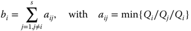
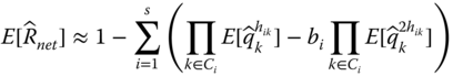
Let Ci be the minimum cut set i for i = 1, 2, …, s of a network system and k be the index for the component type in the network for k = 1, 2, …, n. Let hik be the number of component type k within cut set Ci, where hik ∈ {1, 2, …}. For example, the minimum cut sets of the bridge network is given in Table 2.6, where s = 4 and hik = 1 for all i and k. Let qk be the unreliability estimate of component type k and qk = 1 − rk. When the network has moderate or high reliability, the terminal‐pair reliability, Rnet, can be approximated by the following linear‐quartic function (Jin and Coit 2003):

with

Since terminal‐pair reliability is approximated using the linear and quadratic terms of Qi, this approach is referred to as the linear‐quadratic reliability (LQR) model. Though the LQR model is built upon minimum cuts, due to the truncation of higher‐order terms, it may not always guarantee the lower bound in the entire reliability range. However, when components or network reliability are high, which is true for most real‐world applications, this situation rarely occurs.
2.7.5 Moments of Terminal‐Pair Reliability Estimate
The network reliability estimate, ![]() , is obtained by substituting qk with
, is obtained by substituting qk with ![]() in Eq. 2.7.4. Furthermore, the mean and the variance of
in Eq. 2.7.4. Furthermore, the mean and the variance of ![]() are obtained as follows:
are obtained as follows:

Both equations are obtained by realizing that reliability estimates for different component types are statistically independent. However, the advantages of the LQR model lies in the accommodation of dependency of duplicated components of the same types that appear in multiple cut sets. Take the example of the bridge network in Figure 2.15; the same unreliability estimate for component 1 appears in two MC sets of {1, 2} and {1, 3, 5}. Iterations are required in order to determine the higher‐order moments of component unreliability estimates based on their lower‐order moments (Jin and Coit 2001). Once the higher‐order moments of ![]() are obtained, they are substituted into Eqs. 2.7.7 and 2.7.8 to compute the mean and the variance of the terminal‐pair reliability.
are obtained, they are substituted into Eqs. 2.7.7 and 2.7.8 to compute the mean and the variance of the terminal‐pair reliability.
2.8 Reliability Confidence Intervals
2.8.1 Confidence Interval for Pass/Fail Tests
When a component or a system is being tested, the true probability of the success, r, is usually not known. Here t is suppressed simply for simplicity. If ![]() represents the estimate of r, the simplest and most commonly used confidence interval (CI) for
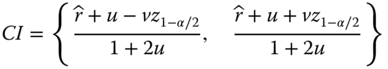
represents the estimate of r, the simplest and most commonly used confidence interval (CI) for ![]() is the normal distribution approximation method. The formula for this method is (Easterling 1972)
is the normal distribution approximation method. The formula for this method is (Easterling 1972)
where z1 − α/2 is the (1 − α/2) × 100 percentile of a standard normal distribution and ![]() and
and ![]() are the sample mean and the variance of
are the sample mean and the variance of ![]() , respectively. However, Eq. 2.8.1 is not valid in extreme cases such as
, respectively. However, Eq. 2.8.1 is not valid in extreme cases such as ![]() = 0 or 1. The latter occurs where zero failures are observed in the test. To overcome the drawback, different methods have been proposed. Among these methods, the Clopper–Pearson interval (Clopper and Pearson 1934) and the Wilson score interval (Wilson 1927) are the two most popular ones. The Wilson score interval estimates are given as
= 0 or 1. The latter occurs where zero failures are observed in the test. To overcome the drawback, different methods have been proposed. Among these methods, the Clopper–Pearson interval (Clopper and Pearson 1934) and the Wilson score interval (Wilson 1927) are the two most popular ones. The Wilson score interval estimates are given as
where

Note that n is the sample size and Eq. 2.8.2 is also valid for a small number of trials and extreme values such as ![]() = 0 or 1.
= 0 or 1.
Realizing that Eqs. 2.8.1 and 2.8.2 are approximation methods, Clopper and Pearson (1934) developed an exact method based on the binomial distribution. The lower and upper reliability bounds, denoted as ![]() and
and ![]() , can be estimated by
, can be estimated by


For the binominal reliability test, k is the number of survivals among n sample units. The Clopper–Pearson bound is also known as the “exact” bound or beta‐binomial bound because there are no underlying distribution assumptions on the reliability estimate ![]() (Vollset 1993).
(Vollset 1993).
2.8.2 Confidence Intervals for System Reliability
For a complex system with multiple subsystems connected in series, the system reliability Rs(t) is the multiplication of subsystem reliability values. Assuming that subsystems fail independently, this implies that the logarithm of the system reliability is the sum of the logarithm of individual subsystem reliability; that is,
where ![]() is the reliability estimate of subsystem i and m is the number of subsystems. If m is sufficiently large, the central limit theorem (CLT) can be involved. CLT states that the sum of a large number of independent random variables tends to be normally distributed regardless of the distribution of individual random variables. In other words, if m is sufficiently large,
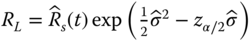
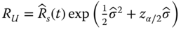
is the reliability estimate of subsystem i and m is the number of subsystems. If m is sufficiently large, the central limit theorem (CLT) can be involved. CLT states that the sum of a large number of independent random variables tends to be normally distributed regardless of the distribution of individual random variables. In other words, if m is sufficiently large, ![]() approximately follows the normal distribution regardless of the subsystem reliability data type or time‐to‐failure distribution. The lognormal based lower and upper reliability bounds, denoted as RL and RU, developed by Coit (1997), are restated below:
approximately follows the normal distribution regardless of the subsystem reliability data type or time‐to‐failure distribution. The lognormal based lower and upper reliability bounds, denoted as RL and RU, developed by Coit (1997), are restated below:
where

where ![]() can be estimated from Eq. 2.3.11. Coit (1997) showed that this approximation is reasonably accurate for any type of complex systems that can be partitioned into at least five series or parallel subsystems. This requirement is usually met for most engineering design problems. For example, a modern wind turbine system typically consists of three blades, a gearbox, a main shaft, DC–AC converters, a generator, and some control and protection subsystems. Each of these functions can be provided by a variety of different components. For instance, a subsystem can be configured as redundant structures, but each function is required at the system level, thereby forming a series model at the system level. The lower and upper bounds of Eqs. 2.8.8 and 2.8.9 can be extended to a parallel system with multiple subsystems where the unreliability can be approximated by a lognormal distribution.
can be estimated from Eq. 2.3.11. Coit (1997) showed that this approximation is reasonably accurate for any type of complex systems that can be partitioned into at least five series or parallel subsystems. This requirement is usually met for most engineering design problems. For example, a modern wind turbine system typically consists of three blades, a gearbox, a main shaft, DC–AC converters, a generator, and some control and protection subsystems. Each of these functions can be provided by a variety of different components. For instance, a subsystem can be configured as redundant structures, but each function is required at the system level, thereby forming a series model at the system level. The lower and upper bounds of Eqs. 2.8.8 and 2.8.9 can be extended to a parallel system with multiple subsystems where the unreliability can be approximated by a lognormal distribution.
2.9 Reliability of Multistate Systems
2.9.1 Series or Parallel Systems with Three‐State Components
Most of the reliability literature deals with binary systems of binary components in which the only two states are functioning and failed. The ideal of a multistate system (MSS) reliability dates back to the early works by Barlow and Wu (1978), El‐Neweihi et al. (1978), and Ross (1979) in the 1970s. These researchers treat the general case of more than two states of components and systems in many practical applications. This idea is useful because in many real‐life situations components and/or systems can operate in intermediate states. For example, a diode allows the current to pass if positive voltage is applied to the P–N junction. It is also capable of blocking the current flow if negative voltage is applied to the junction. Hence, the diode possesses two operating states: it may fail open when forward current is applied or fail short if reverse voltage is applied. Another example is the highway lanes. The actual capacity of a multilane highway reduces if one lane is blocked due to an accident, yet incoming vehicles are still able to go through other lanes at a reduced capacity. In the wind power industry, depending on wind speed, a wind turbine can operate in one of four states: idle, nonlinear power generation, constant power output, and shut‐down states. These are just a few examples of MSSs that are around us. Recent researchers extended the multistate concepts to solving general multistate network reliability problems using the sum of disjoint products (Zuo et al. 2007; Yeh 2007), fuzzy theory (Liu et al. 2008), and supply chain networks (Lin 2009), where the link capacity is characterized as a multilevel reliability index. Xing and Dai (2009) also generalized and extended the decision diagram method to multistate systems.
For an m‐components series system where each component possesses three states, fail open, fail short, and operational, the system reliability can be estimated as (Elsayed 2012)

where ![]() and
and ![]() are the probabilities of fail open and fail short, respectively, at time t. It is worth mentioning that for a multistate series system, the system fails if all m components fail in short mode or any component fails in open mode.
are the probabilities of fail open and fail short, respectively, at time t. It is worth mentioning that for a multistate series system, the system fails if all m components fail in short mode or any component fails in open mode.
The reliability of a parallel system is similar where components possess three states: fail open, fail short, and operational (Elsayed 2012). For a three‐state parallel system, the system fails if all m components fail in open mode or any component fails in short mode:

2.9.2 Universal Generating Function
The universal generating function (UGF) is shown to be quite effective in reliability analysis of components or systems with more than three states. The concept of UGF was introduced by Ushakov (1986). Lisnianski et al. (1996) first applied UGF to analyze power system reliability considering multiple operating states. Levitin et al. (1998) presented an algorithm for optimizing reliability of complex multistate, series–parallel systems with propagated failures and imperfect protections. Ding et al. (2011) performed a long‐term reserve planning by utilizing UGF methods for electric grid with high wind power penetration.
Let s be the number of possible states for component i and j be the index of the state of that component. Furthermore, let pij be the probability of component i in state j for j = 0, 1, …, s − 1. The reliability of the ith multistate component (for i = 1, 2, …, m) in a system can be expressed by a u‐function as follows:
For example, the u‐function of a binary component is u(z) = p1z0 + (1 − p1)z1. For a system with m components, the u‐functions of individual components represent the probability mass function (PMF) of discrete random variables X1, X2,…, Xm. Given the system structure function and u‐functions of components, we can obtain the u‐function that represents the PMF of the system state variable X using the composition operator. That is,
The system reliability measure can be obtained as E[X] = U′(z = 1).
2.10 Reliability Importance
2.10.1 Marginal Reliability Importance
When engineers design a multicomponents system, it is useful to identify the components that are the most crucial to the system reliability. Therefore, it is necessary to define the measurements of the importance of a component to system reliability. The most fundamental measure of statistical importance of components is the Birnbaum importance (BI) measure (Barlow and Proschan, 1975; Leemis 1995). Since its inception, various importance measures haven been developed, such as the Bayesian importance measure, criticality importance measure, redundancy importance measures, and Fussell–Vesely (FV) importance measure. In general, BI and all its extensions can be categorized as marginal reliability importance (MRI) measures as opposed to joint reliability importance (JRI) measures. This section introduces several MRI measures and the concept of JRI will be elaborated in Section 2.10.2. For a comprehensive treatment of reliability importance measures and their applications, readers are referred to the book by Kuo and Zhu (2012b).
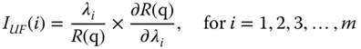
For a system with n independent components, the BI of component i, denoted as IB(i), is defined as
R(r) is the system reliability expressed as a function of component reliability, and r = [r1, r2, …, rm]. If the system consists of several subsystems and each subsystem contains multiple components, then the system reliability importance can also be expressed as
where Ri is the reliability of the ith subsystem and rij is the reliability of the jth component in subsystem i. This “chain‐rule” property makes it possible to compute the importance of each component of a subsystem. To use this formula, the statistical independence of component reliability estimates is required.
Lambert (1975) proposed an upgrading function defined as the fractional reduction in the probability of the system failure when the component failure rate is reduced fractionally. The model assumes an exponential time‐to‐failure for all components and the importance measure is defined as
where λi is the exponential failure rate of component I and q = (q1, q2, q3, …, qm) with qi being the unreliability for component i.
Gandini (1990) proposed the critical importance. This importance measure is based on the fact that it is more difficult to improve the more reliable components than the less reliable ones,

Based on Birnbaum's definition, Griffith (1985) developed a simple sensitivity measure formula for a consecutive k‐out‐of‐n:F system. Papastavridis (1987) also derived the same formula using a different approach. Their formula is given as follows:

where R(i − 1) is reliability of a consecutive k‐out‐of‐(i − 1):F system comprised of components 1, 2, …, i − 1. In addition, R′(n − i) is the reliability of a consecutive k‐out‐of‐(i − 1):F system comprised of components i + 1, i + 2, …, n.
2.10.2 Joint Reliability Importance Measure
B‐importance measures and their extensions do not explain how components mutually affect the system reliability. Design engineers working within a fixed budget might need to conduct a trade‐off analysis among components within a system. Using MRI alone would require calculation of MRI for all components in every trade‐off being considered. The joint reliability importance (JRI) of pairs of components, introduced by Hong and Lie (1993), is more effective for making this kind of trade‐off because it indicates how components mutually interact to the system reliability. The definition of JRI is given as follows:
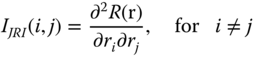
If IJRI(i, j) ≥ 0, this implies that ri is more important when rj is working than when rj has failed. If IJRI(i, j) ≤ 0, this implies that ri is more important when rj has failed than when rj is working. This indicates that IJRI(i, j) is an appropriate metric to quantify the interactions of two components with respect to the system reliability. Later, Armstrong (1995) extended the JRI to cases where component failures are statistically dependent. He showed that similar results hold in more general cases when component failures are statistically dependent.
There are other important contributions in developing reliability sensitivity measures, such as in the context of a network structure (Gertsbakh and Shpungin 2008). Most research has assumed that component reliability values are known exactly. In practice, consideration of component reliability estimation variability may lead to different assessments of the importance of the components.
2.10.3 Integrated Importance Measure for Multistate System
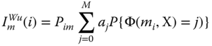
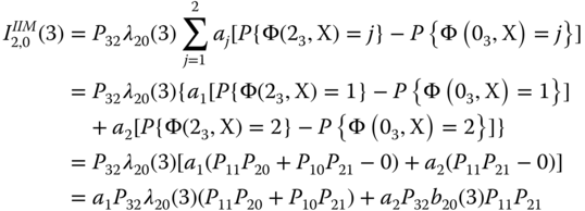
The performance measure of a multistate system aims to assess all outcomes or aspects when both the system and its components may assume more than two levels of reliability states. For example, 0%, 50%, and 100% capacities of a water plant correspond to states 0, 1, and 2, respectively. For a system with n components and M system states, the system performance can be expressed as an expectation of utilities as follows:
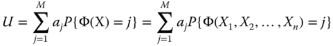
where aj is the system performance level when it is in state j and X = [X1, X2, …, Xn] with Xi being the state of component i. The probability that the system is in state j is given by P{Φ(X) = j}, where Φ(X) is the system structure function related to states of all components. Griffith (1980) proposed the following model to evaluate the importance of state m of component i to the overall system. That is,
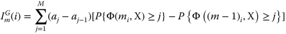
Equation 2.10.8 can be interpreted as the change of the system performance when component i deteriorates from current state m down to adjacent state m − 1.
However, it is more reasonable in practice that a component may transit from state m to any other degradation states, other than state m − 1. To generalize ImG(i), Wu and Chan (2003) proposed a new importance measure that allows the arbitrary transition of component i to any degraded state as
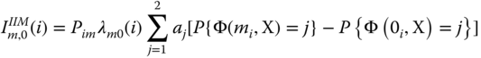
In practice changes in the operating condition usually lead to the change of transition rates of a multistate component. For example, improvements of the repair service or the reduction of usage can affect the transition rates between a degradation state and a fully operable state. Therefore, in the operation and optimization of multistate systems, it is imperative to consider the difference of transition rates between component states. Considering the joint effect of the probability distributions, transition intensities of the target component states and the system performance, Si et al. (2012) proposed the following integrated importance measure (IIM) to study how the transition of component states affects the system performance:

where Pim is the probability that component i is in state m and λml(i) is its transition rate from state m to state l.
We can interpret ![]() as the change of the system performance when component i transfers from state m to state l. IIM can identify which component state holds the largest responsibility of system performance loss and which state should be prioritized in order to improve the system reliability. We take a three‐component system in Figure 2.23 to illustrate how to use the UGF method for IIM evaluation. Note that the state spaces of components 1 and 2 are {0, 1} and the state space of component 3 is {0, 1, 2}. The structure function is Φ(X) = Φ(X1, X2, X3) = min {X1 + X2, X3}. We can define the UGF of component i as follows:
as the change of the system performance when component i transfers from state m to state l. IIM can identify which component state holds the largest responsibility of system performance loss and which state should be prioritized in order to improve the system reliability. We take a three‐component system in Figure 2.23 to illustrate how to use the UGF method for IIM evaluation. Note that the state spaces of components 1 and 2 are {0, 1} and the state space of component 3 is {0, 1, 2}. The structure function is Φ(X) = Φ(X1, X2, X3) = min {X1 + X2, X3}. We can define the UGF of component i as follows:

Figure 2.23A series–parallel system with three components.
By applying the composition operators Φ1, 2 = x1 + x2 and ΦS = min {Φ1, 2, x3} to the three‐component system, the UGF for the entire multistate system is obtained as
In order to find the UGF for the parallel subsystem comprised of components 1 and 2, the operator Φ1, 2 is applied to individual UGF u1(z) and u2(z). It yields
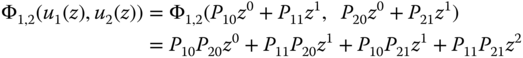
In order to find the UGF for the entire system in which component 3 is connected in series with components 1 and 2 that are configured in parallel, operator ΦS should be applied:
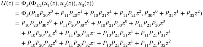
Based on Eq. 2.10.10, the IIM of this simple multistate system can be converted to
The value of P{Φ(mi, X) = j} is equal to the coefficient of zj, which includes Pim > 0 and Pim = 1. For example, we have
Other important measures pertaining to multistate systems are also proposed in the literature. For instance, Ramirez‐Marquez and Coit (2005) develop composite importance measures that are involved in measuring how a specific component affects multistate system reliability. Others (Levitin et al. 2003) have focused on investigating how a particular component state or set of states affects multistate system reliability. Readers can refer to the recent review paper by Kuo and Zhu (2012a) who reported the latest development in reliability importance measures of multistate systems.
2.10.4 Integrated Importance Measure for System Lifetime
System lifetime can be divided into several different stages depending on the characteristics of the failure intensity function or hazard rate curve. The importance of a component to the system reliability performance can also be different in different stages. To achieve the best system performance, the fact that the importance of a component to the system performance may change with the lifetime needs to be taken into account. It is usually not easy to explicitly measure the contribution of component reliability to the system performance in different life stages. However, the change of system performance caused by component degradation is often related to the expected number of component failures. The latter can be predicted by the renewal function. Dui et al. (2014) extended the IIM from a single time instance to different lifetime stages as follows:
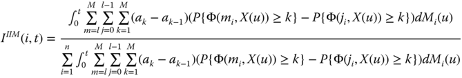
where Mi(t) is the renewal function for component i and dMi(t) is the probability that component i fails in an infinitesimal interval of [t, t + dt]. This generalized IIM describes which component is the most important in improving the system performance across its lifetime or at different stages. The effect of component reliability change on system performance represents a time‐dependent importance measure. It is very useful for system design and maintenance planning. For example, in the design phase, this measure can be a useful tool to determine which components should be prioritized for reliability growth or maintenance support such that the best system performance across different life stages is ensured.
If we let t → ∞ in the upper limit of the integrals in Eq. 2.10.16, the probability that component i causes the system performance reduction is given by

Equation 2.10.17 evaluates the importance of component i that causes the system performance reduction from the time when the system is in a perfect condition to the time when it eventually fails. During the system lifetime, IIIM(i) is a useful metric to determine which components should be managed in terms of lifecycle reliability.
The operation of some systems like satellites contains several missions or stages, such as the launch stage, mission stage, maintenance stage, and re‐entry stage; thus the importance of a component to system performance reduction may vary in different stages. Let t1 and t2 represent the start and the end time of a particular stage, respectively. We can obtain the importance of component i in stage t1 ≤ t ≤ t2 as follows:

The importance measure in different stages is a useful guideline for managers to implement the proper actions for achieving system performance improvement at different life stages. In different life stages, the IIM of component i is only dependent on t1 and t2. By changing the lower or upper time limit, we can easily estimate IIM and characterize its properties in different stages.
References
- Amari, S.V., Pham, H., and Misra, R.B. (2012). Reliability characteristics of k‐out‐of‐n warm standby systems. IEEE Transactions on Reliability 61 (4): 1007–1018.
- Armstrong, M. (1995). Joint reliability importance of components. IEEE Transaction on Reliability 44 (3): 408–412.
- Ball, M.O. (1986). Computational complexity of network reliability analysis: an overview. IEEE Transaction on Reliability 35 (3): 230–239.
- Barlow, R.E. and Proschan, F. (1975). Statistical Theory of Reliability and Life Testing. New York: Holt, Rinehart and Winston.
- Barlow, R.E. and Wu, A.S. (1978). Coherent systems with multi‐state components. Mathematical Operations Research 3 (4): 275–281.
- Borgonov, E. (2007). A new uncertainty measure. Reliability Engineering and System Safety 92 (6): 771–784.
- Clopper, C. and Pearson, S. (1934). The use of confidence or fiducial limits illustrated in the case of the binomial. Biometrika 26 (4): 404–413.
- Coit, D.W. (1997). System reliability confidence intervals for complex systems with estimated component reliability. IEEE Transactions on Reliability 46 (4): 487–493.
- Colbourn, C.J. (1987). The Combinatorics of Network Reliability. New York, NY: Oxford University Press.
- Ding, Y., Wang, P., Goel, L. et al. (2011). Long‐term reserve expansion of power systems with high wind power penetration using universal generating function methods. IEEE Transactions on Power System 26 (2): 766–774.
- Dui, H., Si, S., Cui, L. et al. (2014). Component importance for multi‐state system lifetimes with renewal functions. IEEE Transactions on Reliability 63 (1): 105–117.
- Easterling, R.G. (1972, 1972). Approximate confidence limits for system reliability. Journal of the American Statistical Association 67 (337): 220–222.
- El‐Neweihi, E., Proschan, F., and Sethuramn, J. (1978). Multi‐state coherent systems. Journal of Applied Probability 15: 675–688.
- Elsayed, E.A. (2012). Reliability Engineering, Chapter 2, 2e. Hoboken, NJ: Wiley.
- Gandini, A. (1990). Importance and sensitivity analysis in assessing system reliability. IEEE Transaction on Reliability 39 (1): 61–69.
- Gertsbakh, I. and Shpungin, Y. (2008). Network reliability importance measures: combinatorics and Monte Carlo based computations. WSEAS Transactions on Computers 7 (4): 216–227.
- Goodman, L. (1960). On the exact variance of product. Journal of American Statistical Association 50 (292): 708–713.
- Griffith, W.S. (1980). Multistate reliability models. Journal of Applied Probability 17 (3): 735–744.
- Griffith, W.S. (1985). Consecutive k‐out‐of‐n:F system: reliability, availability, component importance and multi‐state extension. American Journal of Mathematical and Management Science 5 (1 and 2): 125–160.
- Hong, J.S. and Lie, C.H. (1993). Joint reliability‐importance of two edges in an undirected network. IEEE Transaction on Reliability 42 (1): 17–23.
- Jin, T. and Coit, D. (2001). Variance of system reliability estimation with arbitrarily repeated components. IEEE Transactions on Reliability 50 (4): 409–413.
- Jin, T. and Coit, D. (2003). Approximating network reliability estimates using linear and quadratic unreliability of minimal cuts. Reliability Engineering and System Safety 82 (1): 41–48.
- Jin, T. and Coit, D. (2008). Unbiased variance estimates for system reliability estimate using block decompositions. IEEE Transactions on Reliability 57 (3): 458–464.
- Kuo, W. and Zhu, X. (2012a). Some recent advances on importance measures in reliability. IEEE Transactions on Reliability 61 (2): 344–360.
- Kuo, W. and Zhu, X. (2012b). Importance Measures in Reliability, Risk, and Optimization: Principles and Applications, 1e. Wiley.
- Lambert, H. E., Fault Tree for Decision Making in System Analysis, PhD Thesis, UCRL‐51829, University of California, Livermore, 1975.
- Leemis, L.M. (1995). Reliability Probabilistic Models and Statistical Methods. Englewood Clifs, NJ: Prentice Hall, Inc.
- Levitin, G. and Lisnianski, A. (2001). A new approach to solving problems of multi‐state system reliability optimization. Quality and Reliability Engineering International 17 (2): 93–104.
- Levitin, G., Lisnianski, A., Ben‐Haim, H., and Elmakis, D. (1998). Redundancy optimization for series‐parallel multi‐state systems. IEEE Transactions on Reliability 47 (2): 165–172.
- Levitin, G., Podofillini, L., and Zio, E. (2003). Generalised importance measures for multi‐state elements based on performance level restrictions. Reliability Engineering and System Safety 82 (3): 287–298.
- Li, Y.‐F. and Zio, E. (2012). Uncertainty analysis of the adequacy assessment model of a distributed generation system. Renewable Energy 41: 235–244.
- Li, Y.‐F., Ding, Y., and Zio, E. (2014). Random fuzzy extension of the universal generating function approach for the reliability assessment of multi‐state systems under aleatory and epistemic uncertainties. IEEE Transactions on Reliability 63 (1): 13–25.
- Lin, Y.K. (2009). System reliability evaluation for a multistate supply chain network with failure nodes by using minimal paths. IEEE Transactions on Reliability 58 (1): 34–40.
- Lisnianski, A., Levitin, G., Ben‐Haim, H., and Elmakis, D. (1996). Power system structure optimization subject to reliability constraints. Electric Power Systems Research 39 (2): 145–152.
- Liu, Y., Huang, H.‐Z., and Levitin, G. (2008). Reliability and performance assessment for fuzzy multi‐state elements. Proceedings of the Institution of Mechanical Engineers, Part O: Journal of Risk and Reliability 222 (4): 675–686.
- NERC, Reliability Standards for the Bulk Electric Systems of North America, Report of North America Reliability Corporation, January 26, 2017, available at: http://www.nerc.com/pa/Stand/Reliability%20Standards%20Complete%20Set/RSCompleteSet.pdf (accessed on February 12, 2017).
- Papastavridis, S. (1987). The most important component in a consecutive k‐out‐of‐n:F system. IEEE Transaction on Reliability 36 (2): 266–268.
- Ramirez‐Marquez, J.E. and Coit, D.W. (2005). Composite importance measures for multi‐state systems with multi‐state components. IEEE Transactions on Reliability 54 (3): 517–529.
- Ramirez‐Marquez, J.E. and Jiang, W. (2006). An improved confidence bounds for system reliability. IEEE Transactions on Reliability 55 (1): 26–36.
- Ross, S. (1979). Multivalued state component systems. Annual Probability. 7 (2): 379–383.
- Shier, D. (1991). Network Reliability and Algebraic Structures. New York, NY: Clarendon Press.
- Si, S., Dui, H., Zhao, X. et al. (2012). Integrated importance measure of component states based on loss of system performance. IEEE Transactions on Reliability 6 (1): 192–202.
- Taboada, H., Z. Xiong, T. Jin, and J. Jimenez, (2012), “Exploring a solar photovoltaic‐based energy solution for green manufacturing industry,” in Proceedings of IEEE Conference on Automation Science and Engineering, pp. 40–45.
- Ushakov, I. (1986). Universal generating function. Soviet Journal Computer Systems Science 24 (5): 118–129.
- Vollset, S.E. (1993). Confidence intervals for a binomial proportion. Statistics in Medicine 12 (9): 809–824.
- Wilson, E.B. (1927). Probable inference, the law of succession, and statistical inference. Journal of the American Statistical Association 22: 209–212.
- Wu, S. and Chan, L.Y. (2003). Performance utility‐analysis of multi‐state systems. IEEE Transactions on Reliability 52 (1): 14–20.
- Wu, X., Hillston, J., and Feng, C. (2017). Availability modeling of generalized k‐out‐of‐n:G warm standby systems with PEPA. IEEE Transactions on Systems, Man, and Cybernetics: Systems 47 (12): 3177–3188.
- Xing, L. and Dai, Y.S. (2009). A new decision‐diagram‐based method for efficient analysis on multistate systems. IEEE Transactions on Dependable and Secure Computing 6 (3): 161–174.
- Yeh, W.C. (2007). An improved sum‐of‐disjoint‐products technique for the symbolic network reliability analysis with known minimal paths. Reliability Engineering and System Safety 92 (2): 260–268.
- Zuo, M.J., Tian, Z., and Huang, H.‐Z. (2007). An efficient method for reliability evaluation of multistate networks given all minimal path vectors. IIE Transactions 39 (8): 811–817.
Problems
An electric vehicle manufacturer is testing a new generation of lithium‐ion batteries. One hundred battery cells are tested under fast direct current charging and discharging process for 500 cycles. A battery cell fails if its maximum state‐of‐charge (SOC) drops below 80% of its initial capacity. The number of failed cells at 300 and 500 cycles is 10 and 25, respectively. Estimate the mean and the variance of the cell reliability.
- Problem 2.2 Problem Solar PV systems emerged as a green and sustainable energy source to mitigate climate change resulting from carbon emissions. A roof‐top PV system usually consists of PV panels, a charge controller, a battery pack, and a DC–AC inverter. A PV system can also operate in islanding mode like a microgrid if the generation can fully meet the demand. Assume the lifetimes of the PV, the charger controller, the battery, and the inverter follow the exponential distribution with failure rates of 0.1, 0.01, 0.05, and 0.02 failures/year, respectively.
Questions:
- (1) Draw the reliability block diagram of the roof‐top PV system.
- (2) Estimate the reliability of each components at t = 1, 10, and 20 years.
- (3) Estimatestimate the reliability of the entire PV system at t = 1, 10, and 20 years.
- Problem 2.3 Problem A company developed a new microdevice that will be used in offshore oil drilling equipment. To mimic the harsh field operating condition, 20 units are chosen and placed in an environmental chamber to perform accelerated life testing. The following results are observed: one unit failed at t = 60 hours, another unit failed at t = 80 hours, and two additional units failed at t = 90 hours. The test terminated at t = 100 hours with a total of 16 units surviving. Answer the following:
- (1) Estimate the mean and the variance of device reliability at t = 50, 70, and 100 hours, respectively.
- (2) If 10 such devices are deployed in the field, what is the probability that exactly 8 units can survive at t = 70 hours?
- (3) If 10 such devices are deployed in the field, what is the probability that all these units will fail at t = 100 hours.
- Problem 2.4 Problem A system consists of six components connected in series. Reliability tests are applied to these components over a 20‐day period and the results are summarized in Table 2.8.
Table 2.8 Component failure data.
Component type i = 1 i = 2 i = 3 i = 4 i = 5 i = 6 Sample size 20 30 25 16 25 16 Cumulative failures by day 10 0 2 1 1 1 1 Cumulative failures by day 20 1 2 2 1 2 1 Questions:
- (1) Estimate the mean and the variance of the system reliability at t = 10 days.
- (2) Estimate the mean and the variance of the system reliability at t = 15 days.
- (3) Estimate the mean and the variance of the system reliability at t = 20 days.
- Problem 2.5 Problem Let
 be the unreliability estimate of a component and
  = 1 −
= 1 −  . Show that
  .
. - Problem 2.6 Problem A series system consists of five components. Estimate the mean and the variance of the reliability estimates of the series system at t1 = 1 week and t2 = 2 weeks, respectively. Note that component lifetime testing data are presented in Table 2.9.
Table 2.9 Component lifetime testing data. i 1 2 3 4 5 Sample size 10 14 20 17 19 Failures by t1 0 1 2 1 0 Failures by t2 1 2 2 1 1 - Problem 2.7 Problem Show that
 in Eq. 2.3.3 is an unbiased estimate of Rs(t).
 - Problem 2.8 Problem Show that
 in Eq. 2.3.11 is an unbiased estimate of
  .
. - Problem 2.9 Problem For aircraft equipped with two identical engines, the system is reliable as long as one engine is functional. What is the minimum reliability requirement for each engine in order to attain the 0.999 999 reliability goal of the aircraft? What is the aircraft reliability if three engines are installed?
- Problem 2.10 Problem The same group of components in Problem 2.6 are used to construct a parallel system. Estimate the mean and the variance of the reliability estimates of a system comprised of five components in parallel at t1 and t2, respectively.
- Problem 2.11 Problem Show that Eqs. 2.4.2 and 2.4.3 are the unbiased estimates for
 and
and  , respectively. Note that
  is the reliability estimate for a parallel system.
 - Problem 2.12 Problem Based on the reliability data in Example 2.1, assume that a battery storage system is comprised of three battery cells connected in parallel. The battery system is able to discharge the electric energy as long as one cell is functional. Evaluate the reliability of this energy storage system in terms of mean reliability and its variance using Monte Carlo simulations.
- Problem 2.13 Problem Show that series and parallel systems are the special cases of k‐out‐of‐n:G systems. If k = n, Eq. 2.6.1 is equivalent to Eq. 2.3.3 for a pure series system reliability model. If k = 1, it is the same as Eq. 2.4.1 for pure parallel systems.
- Problem 2.14 Problem A power grid is often designed under N − 1 redundancy criterion, meaning the network is able to meet the peak load even if one generator fails or is unavailable due to maintenance. Suppose the peak load of the power grid is 200 MW (megawatts) and 10 identical power generators are installed to produce the electricity for industrial, commercial, and residential users. The power capacity of each generator is 25 MW. Answer the following questions:
- Assuming 10 generators are always available and never fail, is this power system indeed an N − 1 design scheme?
- If the reliability of each generator is 0.99 and the reliability of the power grid is required to be 0.9999, is this power system an N − 1 design scheme?
- Given that the reliability of each generator is 0.99 and the power system is designed under the N − 1 rule, what is the maximum reliability that the grid can achieve in peak hours?
- Problem 2.15 Problem Estimate the mean and the variance of the following series–parallel and parallel–series system based on component reliability data in Table 2.5 (Figure 2.24).
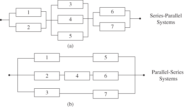
Figure 2.24(a) Series–parallel system, (b) parallel–series system. - Problem 2.16 Problem Please estimate the mean and the variance of the following hybrid system based on component reliability data in Table 2.5 (Figure 2.25).
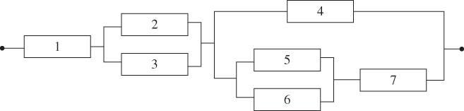
Figure 2.25A mixed series–parallel system. - Problem 2.17 Problem It is anticipated that by 2030 wind energy will represent 30% of the utility market in the USA. To achieve this penetration rate, large wind farms with dozens or hundreds of wind turbines are being deployed in onshore regions or offshore areas. A main challenge in operating a wind farm is the high equipment maintenance costs, which include spare parts, labor hours, and rental of cranes or boats (in offshore). Suppose an offshore wind farm consists of a fleet of 50 wind turbines and the reliability of each wind turbine is r = 0.9 at the end of year 1 and r = 0.75 at the end of year 2. The fleet availability is defined as the probability that a certain number of wind turbines must be functional at any instance of time. Compute the fleet availability if:
- (1) At least 45 wind turbines must be operational during the first year.
- (2) At least 45 wind turbines must be operational during the second year.
- (3) If we want to ensure that at least 45 turbines are available with 0.99 confidence in year 1, what is the minimum reliability of an individual wind turbine?
- Problem 2.18 Problem Find the minimum path and minimum set of the network in Figure 2.1d.
- Problem 2.19 Problem Based on the minimum path and minimum set of the network in Figure 2.1d, compute:
- The terminal pair reliability based on minimum paths.
- The terminal pair reliability based on minimum cuts.
- What is the exact terminal pair reliability of this network (using edge decomposition)?
- Problem 2.20 Problem A diode bridge is a device that changes alternating current (AC) to direct current (DC). Its reliability diagram is shown in Figure 2.15 where components 1–5 correspond to five diodes. A total of 30 devices have been made and installed at the beginning of January 2014. Failures reported from customers are collected and analyzed by the service department of the device manufacturer and the results are summarized in Table 2.10. Please estimate the mean and the variance of this AC–DC device reliability based on the linear‐quadratic reliability model.
Table 2.10 Reported diode failures in each quarter in 2014. Months i = 1 i = 2 i = 3 i = 4 i = 5 1–3 0 0 0 0 1 4–6 1 0 0 0 0 7–9 1 1 1 1 0 10–12 0 1 0 0 1 - Problem 2.21 Problem Let
 be the component reliability estimate. Given the mean
  and the variance
  , estimate the confidence interval for
  based on the normal distribution approximation at α = 0.1 and 0.05, respectively.
 - Problem 2.22 Problem Given
 and the sample size n = 20, estimate the confidence interval for
  using Wilson score interval estimates at α = 0.1 and 0.05, respectively.
 - Problem 2.23 Problem Given
 and the sample size n = 20, estimate the confidence interval of reliability estimate
  using the Clopper–Pearson method at α = 0.1 and 0.05, respectively.
 - Problem 2.24 Problem Based on the system structure and the component reliability given in Problem 2.6, estimate the confidence interval of the system reliability estimate at α = 0.1 and 0.05, respectively. The following approaches can be considered:
- (1) The log‐normal approximation approach.
- (2) Normal approximation.
- (3) How about the beta binomial method (i.e. the Clopper–Pearson method)?
- Problem 2.25 Problem Estimate the reliability of the following two systems shown in Figure 2.26 where each component possesses three states: fail open, fail short, and normal operation. The component reliability information is listed in Table 2.11.
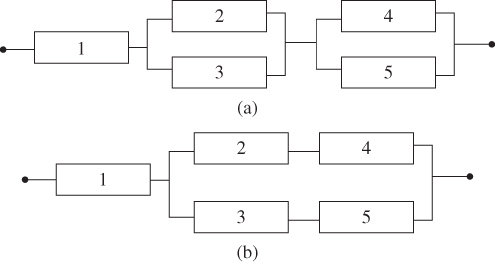
Figure 2.26(a) A series–parallel system, (b) a mixed series–parallel system. Table 2.11 Reliability of multistate components.
i 1 2 3 4 5 Fail open 0.1 0.1 0.1 0.1 0.1 Fail short 0.2 0.2 0.2 0.2 0.2 - Problem 2.26 Problem Three components are available to construct a multistate system and each component can operate in one of following states: 100%, 75%, 5%, or 25% of the capacity. The probabilities associated with each state are given in Table 2.12. Using the universal generating function approach to estimating the MSS reliability, estimate the system reliability if:
- Three components are connected as a pure series system.
- Three components are connected as a pure parallel system.
Table 2.12 Reliability of four‐state components. State (j) j = 1 j = 2 j = 3 j = 4 Capacity (%) 100 75 50 25 Component 1 0.5 0.3 0.1 0.1 Component 2 0.4 0.2 0.2 0.2 Component 3 0.3 0.45 0.1 0.15 - Problem 2.27 Problem Compute the Birnbaun importance measures of each component within a system in Figure 2.27. The reliability of components 1 to 4 is r1 = 0.9, r2 = 0.85, r3 = 0.8, and r4 = 0.75.
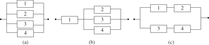
Figure 2.27(a) Parallel system; (b) a series–parallel system; (c) parallel–series system. - Problem 2.28 Problem Show that Eqs. 2.5.1 and 2.5.3 are, respectively, unbiased estimates of
 and
and  , where
  is the reliability estimate of a parallel system.
 - Problem 2.29 Problem Show that Eqs. 2.5.5 and 2.5.6 are, respectively, unbiased estimates of
 and
and  , where
  is the reliability estimate of a series–parallel system.
 - Problem 2.30 Problem For a series system comprised of m components, the mean and variance of
 are μi and
  , where
  is the reliability estimate of component i. Show that the lower and upper bounds of the system reliability estimate,
  , are given as follows:
 where
where
- Problem 2.31 Problem Given is a system with five components configured in parallel. To estimate the system reliability, 20 units of each are placed for reliability testing. The number of failures at t = 50 days and 100 days are recorded and listed in the following table. Assuming the system unreliability is lognormally distributed, estimate the following:
- The mean and the variance of the system reliability estimate at t = 50 and 100 days.
- The lower and upper bounds of the system reliability estimate at t = 50 and 100 days.
Component 1 2 3 4 5 n 20 20 20 20 20 k (t = 50 days) 1 0 2 1 2 k (t = 100 days) 2 1 3 2 2