
5
Accelerated Stress Testing and Economics
5.1 Introduction
In accelerated stress testing (AST), the product undergoes higher‐than‐normal operating conditions in an effort to extrapolate the product reliability in use conditions by precipitating faults in a compressed period. Typical accelerating stresses include environmental, electrical, mechanical, and chemical factors. The choice of accelerating stress levels and the allocation of available test units to these levels are the key considerations in executing accelerated test experiments. This chapter begins with the introduction of the concept of AST that include a highly accelerated life test (HALT) and highly accelerated stress screening (HASS). The reliability extrapolation is often justified on the basis of physical and chimerical laws, or a combination with statistical models derived from the lifetime data. The chapter describes one‐stress Arrhenius law and multistress Eyring models, both of which are physics‐experimental‐based models. We also present three types of statistics‐based AST models: a scale and use rate acceleration model, a non‐parametric model, and semi‐parametric models that include a well‐known proportional hazard model (PHM). Both HALT and HASS are costly to implement due to the consumption of equipment, materials, and labor. Economic models are developed to guide the product manufacturer to realize the cost savings in the deployment of HASS. This chapter concludes by presenting a case study of implementing HASS and environmental stress screening (ESS) to improve the product reliability in a subcontract manufacturing facility.
5.2 Design of Accelerated Stress Test
5.2.1 HALT, HASS, and ESS
Accelerated life stress testing or AST can be simply defined as: applying high levels of stresses to a device under test (DUT) for a short period of time to extrapolate the lifetime of the device in the use condition assuming it will exhibit the same failure mechanisms. Also known as accelerating variables, such stresses include temperature, humidity, voltage, power, speed, mechanical force, and torque, among others. The key here is to understand the root causes of failures and their relation to the applied stresses, either environmental, mechanical, or electrical stresses. The main purpose of AST is to accelerate the reliability growth in the product development stage such that the reliability performance at the time to shipment meets the design requirement. Depending on the stress levels and testing time, two types of AST are generally adopted in industry: HASS and HALT. We elaborate on both techniques below.
As shown in Figure 5.1, the overall operating range of a product can be divided into three areas: product specification, operating margin, and the destructive margin. The product specifications represent the normal stress levels that the product is expected to use in the field. The operating margin formed between the lower (upper) operating limit and the lower (upper) specification limit is the safety area where the product is still able to operate normally, but with a higher failure rate. This is also the operating area of implementing the HASS process, a technique that uses stresses beyond product specifications in order to detect infant mortality failures and shorten the time to corrective actions in mass production.

Figure 5.1ALT and HASS and product design margins.
The destructive margin formed between the lower (upper) destructive limit and the lower (upper) operating limit represents the area where the product operates under a much higher than usual stress, and will fail quickly. This is the testing domain of the HALT process that aims to precipitate the failure modes in a compressed time window. Sometimes HALT is also referred to as the test, analyze, and fix (TAAF) during the product design and development stage.
If a product operates beyond the lower or upper destructive limits, failure will occur immediately because the product suffers from failure mechanisms that may not happen if operating within the destructive margins. Although Figure 5.1 depicts a two‐side (i.e. upper and lower) specification, many products like electronic devices are more susceptible to failures under high temperature and voltage rather than at the low stresses. Mechanical components like bearings and gears are prone to failure only if they are subject to high rotating speeds or torques. Hence both HASS and HALT processes in these circumstances is single‐sided (right) testing rather than two‐sided experimentation.
Both HALT and HASS are discovery testing as compared to compliance testing, like the reliability demonstration test. However, the following distinctions should be made between HASS and HALT. First, HASS is a reliability growth technique incorporated in the production phase to identify manufacturing defects that could cause early infant mortality, while the purpose of HALT is to identify the design flaws or weakness in the early development and prototyping phase. The result of HALT can be applied to the robust product design, like the design of the integrated chip wire‐bonding process that is less susceptible to environmental stresses (Yang and Yang 1999). Second, HASS is a quality control process and applicable to all finished products, while HALT is implemented on sampled products, usually in prototype forms. Third, HASS in general is more economical than HALT because the use of equipment and materials, such as chambers, shakers, instruments, power, and cooling facility (e.g. liquid nitrogen), is less intensive in HASS.
In certain applications where the operating limits are already extreme (i.e. operating margin and product specification overlaps), ESS is often preferred over the HASS process. The key difference is that the stresses applied by ESS are within a product's non‐destructive operating range used in the field. Like HASS, the ESS program is also implemented in post‐production in which 100% of produced units are subjected to more severe stresses than in normal service. However, each method achieves the goal differently, depending on application‐specific timelines, costs, and stress levels.
Other types of filtering processes exist to precipitate early infant mortality, such as burn‐in, thermal cycling, power cycling, and thermal shocks. For instance, Yan and English (1997) proposed a modified bathtub curve that integrates the concept of latent failures and obsolescence for microdevice manufacturing. The idea is to construct an integrated cost model used to determine both optimal burn‐in and ESS times. Ye et al. (2013) design an optimal burn‐in process to minimize the warranty cost of a new product. Like ESS, the stress levels of these techniques are typically set in the boundary between the operating margin and the product specification. Table 5.1 summarizes the applications, stress levels, and impact units of different accelerated testing and screening techniques.
Table 5.1 Summary of HALT, HASS, ESS, and other screening techniques.
| Test type | Application | Stress level, timeframe | Impacts | Purpose | Cost ($/item) |
| HALT | Design, development, and prototyping | Destructive margin, very short time | Small sample | Identify design defect and weakness | High |
| HASS | Production stage | Operating margin | 100% products | Remove latent failure or infant mortality | Medium to low |
| ESS | Production stage | Extreme limits of product specification | 100% products | Remove latent failure, infant mortality, and manufacturing defects | Low |
| Burn‐in, thermal cycling, thermal shock, power cycling, voltage margining | Production stage | Extreme limits of product specification | 100% products | Remove latent failure, infant mortality, and manufacturing defects | Low |
5.2.2 Types of Accelerating Stresses
In an effective accelerated test, the reliability expert chooses one or more stress types that cause the product to fail under normal operating conditions. The stresses are then applied at various accelerated levels and the time‐to‐failure and time‐to‐degradation for the units under test are recorded. For example, a product normally operates at 30 °C ambient temperature with 40% relative humidity (RH). If high temperature and humidity cause the product to fail more quickly, the product can be tested under 60 °C with RH = 70% or 100 °C with RH = 90% in order to accelerate the units to fail more rapidly. In this example, the stress type is temperature and humidity and the accelerated stress levels are 60 and 100 °C for temperature and 70% and 90% for RH. Depending on the nature of product materials and the operating conditions, stresses used to accelerate the failure can be classified into three categories, as shown in Table 5.2. These are environmental, electrical, mechanical, and chemical stresses.
Table 5.2 Classification of stress types and their factors.
| Stress type | Stress factors |
| Environmental | Temperature, thermal cycle, humidity, thermal shock, vibration, sand and dust, nuclear and cosmos radiation, altitude |
| Electrical | Voltage, current, power, frequency, electrical field, power cycling |
| Mechanical | Force, friction, torque, fatigue, vibration, pressure |
| Chemical | Corrosions, diffusions |
5.2.2.1 Environmental Stresses
They are the factors that are closely related to the surroundings of the operating product. Temperature, humidity, and thermal cycling are the typical environmental stresses. It is important to determine the critical environmental stresses and assign appropriate stress levels that do not induce different failure modes other than the ones at the use condition. For instance, the life of semiconductor devices are sensitive to the operating temperature and RH. However, if the same devices are used in satellites or space stations orbiting outside the atmosphere, beta radiation and gamma rays have the ability to ionize semiconductor materials, which results in new failure effects: (i) producing additional electron‐hole pairs and (ii) creating high‐energy charges to be injected into silicon dioxide regions, causing the degradation and failure of transistors. While the humidity emerges as a key environmental stress for electronic devices used in vapor‐intensive tropical areas or rainforest regions, cosmic radiation becomes one of the primary environmental stresses when they are used in space engineering systems.
5.2.2.2 Electrical Stress
Electrical stress is applied to exercise a product near or at its electrical limits. Examples of electrical stress tests include simulating junction temperatures on semiconductors and testing the insulation of circuit breakers of high‐voltage transmission. Two basic types of electrical stress tests are available: voltage margining and power cycling. Voltage margining pertains to varying input current or voltage above and below nominal operating limits. A subset of voltage margining is frequency margining which is often used in stressing the speed (or the clock cycle) of microprocessors like the central processing unit. Other types of voltage margining include electric field. Power cycling consists of turning a machine's power on and off at specified levels with predetermined time intervals. It is often used to induce the solder joint failure by creating thermal fatigue when the temperature of solder joints increases and decreases cyclically with the on–off power. Electrical stress alone is not able to expose the number of defects commonly found under the vibration test or temperature cycling. However, it is often economical to implement the electrical stress along with other stresses to increase the overall effectiveness of ALT or HASS programs. This is because it is often required to supply electric power to products under test in order to stimulate soft or hard failures induced by mechanical or environmental factors.
5.2.2.3 Mechanical Stress
This type of stress can be induced by force, torque, vibration, and thermal shocks, among others. The effort would be caused by internal or external factors. For instance, a solder joint crack in a circuit board is often induced by repetitive thermal cycling, which is an internal factor. The disconnection of a universal serial bus connector in a computer could be caused by frequent insertion and extraction operations, belonging to an external factor. The breakage of wind turbine blades is induced by material fatigue due to vibration and wind shocks repeatedly applied to the blade. Therefore, failure of mechanical systems is largely associated with external factors.
5.2.2.4 Chemical Stress
Corrosion and diffusion are two basic failure mechanisms induced by chemical stresses. Corrosion is a natural process converting a refined metal to a more chemically stable form, such as its oxide, hydroxide, or sulfide. It is the gradual destruction of materials by chemical and/or electrochemical reaction with their environment. Diffusion is the net movement of molecules or atoms from a high concentration region to a low concentration region as a result of random motion of tiny particles. Diffusion is driven by a gradient in the chemical potential of the diffusing species.
5.2.3 Stress Profiling
Different types of load profile are available in AST and their application depends on the stress type, availability of the test bed, and the product's operating condition. Based on the stress amplitude and its variation frequency, stress loading profiles can be classified into five categories: (i) constant stress, (ii) sinusoid stress, (iii) step stress, (iv) ramp‐up and dwell, and (v) zigzag and cyclic stress.
Figure 5.2 depicts the loading profile of a constant stress. As the name implies, the stress level remains constant during the entire test period. For ALT and HASS processes subject to a constant stress level, the decision variables are the level of the stress A1 and the duration of the test period t1. For instance, Yang (1994) proposed an optimal design of four‐level constant‐stress ALT plans that chose the stress levels, test units of each stress, and censoring times to minimize the asymptotic variance of the maximum likelihood estimators of the mean life. Stresses like temperature, humidity, voltage, or power can be set at a fixed level during the accelerated testing period.
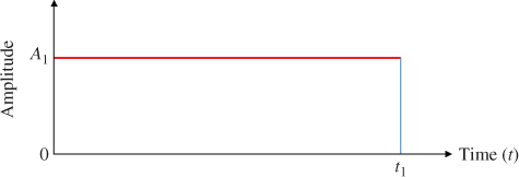
Figure 5.2Constant stress level.
A sinusoid stress profile is constantly used in fatigue testing of mechanical systems. As shown in Figure 5.3, the stress profile is characterized by two parameters: the amplitude A1 and the cycle period T. The mathematical expression of the sinusoid stress is

Figure 5.3Sinusoid stress.
where f is the frequency of stress and f = 1/T is in units of Hertz. Obviously, the frequency and the amplitude are the key factors that determine the severity of the stresses imposed on the testing units.
Figure 5.4 shows a step‐stress loading profile where a constant stress is applied for a period of time and then the stress is escalated to a new level for another period of time. This process is repeated until it reaches the end of the test time or all the stress levels have been applied. The decision variables in a step‐stress test include the number of stress steps and the amplitude and the duration of each step stress. The mathematical formula is

Figure 5.4Step stress (or stair stress).
where t0 = 0 and u(t) is a standard step function with u(t) = 1 for t ≥ 0 or u(t) = 0 for t < 0. For example, for the three‐step stress test in Figure 5.4, the values of A1, A2, A3, t1, t2, and t3 need to be determined prior to the execution of the ALT or HASS test. As an example, Miller and Nelson (1983) designed an optimum plan for two‐step stress tests where all units are run to failure and the goal is to minimize the asymptotic variance of the maximum likelihood estimator of the mean life. In electrical stress testing, it is relatively easy for stresses like voltage, power, and electric field to be transitioned from one level to another instantaneously. Hence the step stress loading profile is commonly adopted in an electrical test.
Figure 5.5 depicts the loading profile of a dwell and ramp‐up stress where the transition from the low stress level to the upper level is not instantaneous, but it takes an amount of time, i.e. t2 − t1 and t4 − t3, before reaching level A2 and A3, respectively. Hence, dwell and ramp‐up profiles are usually applied in environmental tests where different levels of stresses like temperature and humidity cannot be reached immediately due to the limitation of the test equipment.
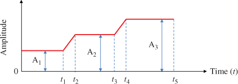
Figure 5.5Dwell and ramp‐up stress.
There exist other types of stress profiles such as the zigzag stress in Figure 5.6 and the cyclic stress in Figure 5.7. These can be treated as the variation of the dwell and ramp‐up stress in Figure 5.5. For instance, in the zigzag stress, there is no dwell period and the stress ramps up from zero to A1 for a period of t1 and the ramps down to level A2 between t1 and t2. This process is repeated until it reaches the end of the test time. The pattern of a cyclic stress test is similar to a zigzag stress profile, except that there exist dwelling periods once the stress reaches the peak or drops to the valley. Cyclic stress profiles are widely used in power cycling of electronics equipment, namely, the products under test undergo a sequence of tests: power‐on at t = 0, warm‐up between 0 and t1, normal operation between t1 and t2, power‐off between t2 and t3, and complete shut‐down from t3 and t4. While A1 > 0, in a power cycling test A2 is usually set to 0.
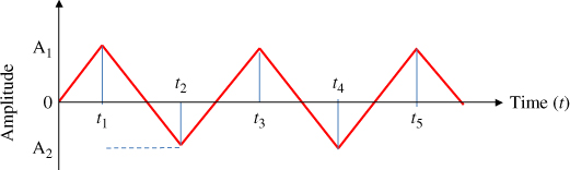
Figure 5.6Zigzag stress profile.

Figure 5.7Cyclic stress profile.
5.3 Scale Acceleration Model and Usage Rate
5.3.1 Exponential Accelerated Failure Time Model
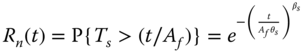
A scale accelerated failure time (SAFT) model belongs to a statistics‐based reliability modeling approach. In an SAFT model, lifetime T(s) at stress s is scaled by a deterministic number that often depends on the applied stresses s and certain unknown parameters. Therefore, the SAFT model in statistical literature is also referred to as the accelerated failure time (AFT) model. Let Tn and Ts be, respectively, the lifetime under the normal use condition and the accelerated stress condition. Their relation is governed by the acceleration factor (AF) as follows:

where Af is the acceleration factor and Tn and Ts are the lifetime at normal and the stressed condition, respectively. Lifetime is accelerated when Af > 1 and decelerated if Af < 1. For example, if the lifetime at the stressed level is exponentially distributed with failure rate λs, then the reliability at stress s is
Let Rn(t) be the reliability at the normal stress sn. Then it can be extrapolated as
Furthermore, the probability density function (PDF) and the hazard rate function at sn can also be obtained as

Equation (5.3.5) shows that the hazard rate (or failure rate) at the normal condition is scaled down by a factor of Af, which echoes the definition of the acceleration factor in Eq. (5.3.1).
5.3.2 Weibull AFT Models
In this section, we extend the exponential AFT model to the two‐parameter Weibull lifetime distributions. Let θs and βs be the Weibull scale and shape parameters under the accelerated condition. Then the reliability function under the stress condition is
Given Rs(t), we can derive the reliability, PDF, and hazard rate in normal use; they are given as follows:


Let θn and βn be, respectively, the scale and shape parameters in normal use. Based on Eqs. (5.3.7–5.3.9), it is also easy to realize that
The above results are based on a common assumption that the applied stress only influences the scale parameter, but not the shape parameter of the distribution (Escobar and Meeker 2006).
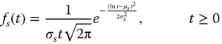
5.3.3 Lognormal AFT Models
Lognormal distribution is widely used for modeling and estimating the failure times of electronics components subject to thermal or electric stresses. These include temperature, voltage, power, and the electric‐magnetic field. Another application of lognormal distribution is to model the fracture of the substrate of integrated circuits. The root cause of this failure mechanism is power cycling. It makes the device junction temperature fluctuate because of the differences between the coefficients of thermal expansion of device packaging materials. Let μs and σs be the parameters of the lognormal distribution under the stressed condition; then the PDF is
The AF condition in Eq. (5.3.11) in logarithmic scale can be expressed as
By substituting Eq. (5.3.12) into Eq. (5.3.11), the PDF at the normal use condition is

where μn and σn are the parameters of the lognormal distribution under normal use conditions. The following relations held for the lognormal AFT model:
The lognormal distribution belongs to the location‐scale distribution family where μn (μs) are called the location parameters that are dependent on stress level s, and σn (σs) are called the scale parameters that are independent of s. Other location‐scale distributions include normal, uniform, and Cauchy distributions.
5.3.4 Linear Usage Acceleration Model
While the product is placed in the normal operating environment, increasing the usage can be an effective approach to accelerating the life as well. This differs from HALT and HASS techniques where operating conditions such as temperature, voltage, and vibrations are escalated to higher than the normal operating condition. Usage acceleration can be applied to products subject to intermittent or non‐continuous operations, such as relays, switches, bearings, motors, gearbox, vehicle tires, washing machines, and air conditioners. The basic assumption of usage acceleration models is that the product useful life should not be affected by the increased rate or cycles of operations during the short time period. This is important because cycling simulates the actual use and if the cycling frequency is low enough, the test units can return to the steady state prior to the start of the next cycle. As such, the time‐to‐failure distribution is independent of the cycling rate or there is no reciprocity effect. The implies that there exists a linear relation between the accelerated lifetime and the lifetime under normal use, namely
The model in Eq. 5.3.16 is also called the SAFT because the lifetime is proportional to the usage rate. For example, Johnston et al. (1979) observed that the cycles‐to‐failure of a type of insulation material was shortened with the increased alternating current (AC) frequency. The acceleration factor can be estimated as Af(412) = 412/60 ≈ 6.87 when the AC frequency in voltage endurance tests was increased from 60 to 412 Hz by keeping the voltage at the same level.
Ideally increasing the usage rate should not significantly change the actual use condition of the product. Hence in accelerated usage rate tests, other relevant factors should be identified and controlled to reflect the actual use environment. If the cycling rate is too high, it can cause reciprocity breakdown (Escobar and Meeker 2006). For example, in a power cycling test excessive heat may build up on test units (e.g. microprocessor chips) if the time interval between two consecutive power cycles are too short. This induces the reciprocity breakdown because the cycles‐to‐failure distribution depends on the cycling rate. Thus, it is necessary to let the test units “cool down” between the cycles of consecutive operations.
5.3.5 Miner's Rule under Cyclic Loading
Most mechanical systems often endure repeated loads that are constantly applied to the object, and the magnitude of the loads may exceed the upper or lower limits of the material strength. The stresses above or below the limits are called critical stresses. Typically examples include wind turbine blades, suspension spring, aircraft wings, and gearbox, among others. Fatigue is generated by cyclic stresses beyond the critical values, especially the upper limit. The system eventually breaks down as the result of the accumulation of fatigues.
Figure 5.10 shows a typical cyclic load profile that fluctuates between the upper and lower limits. It is assumed that there is no fatigue effect as long as the stress does not exceed the critical levels. The fatigue lifetime of an item subject to varying stress can be estimated using Miner's rule. This is expressed as
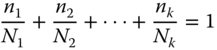
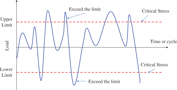
Figure 5.10A typical cyclic load profile for mechanical systems.
where
- ni = the number of cycles at a specific load level (above the fatigue limit)
- Ni = the median number of cycles to failure at that level
- k = the number of the load levels or profiles
The values of Ni for i = 1, 2, …, k can be obtained from the so‐called stress‐cycle curve, or S–N curve. Figure 5.11 depicts the empirical relationship between stress and cycles to fatigue. An important assumption is that the life is infinite below the fatigue limit stress Lc, while the system fails immediately if the maximum stress Lmax is imposed. When the applied stress varies between Lc and Lmax, it induces material fatigue, leading to a failure as a result of cumulative damages.
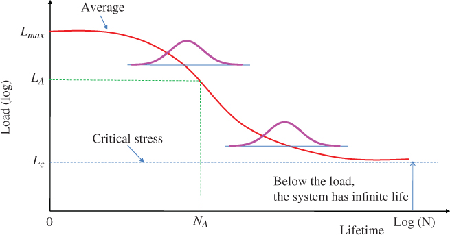
Figure 5.11S–N curve.
5.4 Arrhenius Model
5.4.1 Accelerated Life Factor
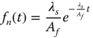
The Arrhenius acceleration model belongs to physics‐experimental‐based models. Proposed by Svante Arrhenius in 1889, the Arrhenius equation is an empirical formula for describing the temperature dependence of reaction rates (Arrhenius 1889). It has been recognized as one of the earliest and most effective acceleration models to predict how the time‐to‐failure changes with the imposed temperature stress. The model has been widely used for failure mechanisms that depend on diffusion processes, migration processes or chemical reactions. Hence, it covers many of the non‐mechanical (or non‐material) fatigu failure modes that are responsible for the dysfunction of electronic circuits or devices. The Arrhenius model takes the following form:
where
T = the temperature measured in degrees Kelvin (K)
Ea = the activation energy in units of electronvolts (eV)
k = Bolztmann's constant with k = 8.617 × 10⁻⁵ eV /K
Parameter A is a non‐thermal constant called the scaling factor. The value of Ea depends on the materials of the product and the failure mechanism. Typically it is in a range between 0.3 and 0.4 eV, but can go up to 1.5 eV or higher. The Arrhenius model argues that for reactants to transform the product into a chemical process, they must first acquire a minimum amount of energy, called the activation energy Ea. The concept of activation energy explains the exponential relationship between the reaction rate and the fraction of molecules having kinetic energy larger than Ea. The latter can be calculated from statistical mechanics.
Under different A and Ea values, Figure 5.12 plots three cases to show how the time‐to‐failure decreases with the elevation of temperature. Note that the vertical axis represents tf(T) in logarithmic scale with base 10. Assume Case 1 as the baseline with A = 0.01 and Ea = 0.3. By comparing Cases 1 with 2, it is found that activation energy plays a critical role in determining the time‐to‐failure (i.e. reliability). If Ea increases from 0.3 to 0.4 with the same A = 0.01, the value of tf(T) in Case 2 increases over 300 times at T = 200 K and 20 times at T = 400 K as opposed to Case 1.

Figure 5.12Time‐to‐failure with different A and Ea.
5.4.2 Other Units for Activation Energy
When dealing with the degradation of organic materials, such as food, plastics, pharmaceuticals, paints, and coatings, it is more common to replace the Boltzmann constant k with the universal gas constant R. Then the Arrhenius model becomes
For example, R = 8.314 46 J /(mol K) is commonly given in units of joules per mole Kelvin. In this formula, Ea is the activation energy in units of joules per mole (J/mol). According to Escobar and Meeker (2006), the corresponding Arrhenius acceleration factor is
where Tn and Ts are the temperature in Kelvin in the use and the stressed condition, respectively.
It is worth mentioning that the Arrhenius model is not applicable to all thermal acceleration problems. A main reason is because both the activation energy Ea and the rate constant k are experimentally determined. They represent macroscopic parameters that are not truly related to threshold energy and the success of individual molecular collisions. Rather, macroscopic measurements are the result of a group of molecular collisions with different parametric scenarios. Nevertheless, the Arrhenius model has been proven to be satisfactorily in many different applications.
5.5 Eyring Model and Power Law Model
5.5.1 Eyring Model
The Eyring model has its theoretical basis in chemical reactions and quantum mechanics. It is a physics‐experimental‐based acceleration model. If an aging process, such as chemical reaction, corrosion, diffusion, or metal migration, is driving the reliability degradation toward failure, the Eyring model is able to capture how the rate of degradation varies with the imposed stress. Unlike the Arrhenius model, the Eyring model can be used to model life acceleration under multiple stresses, includes temperature, voltage, current, and other relevant stresses. A two‐stress Eyring model accommodating temperature and one non‐thermal stress takes the following form (NIST 2017):

where
- T = temperature stress in degrees Kelvin
- S = non‐thermal stress in forms of voltage or current (or a function of voltage or current), or any other relevant stress
- A, B, C, and m = model parameters
As with the Arrhenius model, k is the Boltzmann constant and Ea is the activation energy. Parameters A, B, and m determine the acceleration effect between stressed and use conditions, and C determines the combined effect of stresses T and S. Applications in the literature have typically use a fixed value of m ranging from m = 0 (Boccaletti et al. 1989), m = 0.5 (Klinger 1991a,b), to m = 1 (Mann et al. 1974; Nelson 1990).
If one compares Eq. (5.5.1) with Eq. (5.4.1), the temperature terms are very similar between them, explaining why the Arrhenius model has been so effective in establishing the connection between the parameter Ea and the quantum theory concept of “activation energy needed to cross an energy barrier and initiate a reaction” (NIST 2017). The general Eyring model accommodating temperature and n non‐thermal stress factors can be expressed as

where S = {S1, S2, …, Sn] is the non‐thermal stress vector and Bi and Ci are the parameters associated with stress Si for i = 1, 2, …, n. In the general Eyring model there exist terms characterizing the interactions between the temperature and non‐thermal stresses. This means that the effect of changing temperature on the lifetime depend on the levels of other stresses. In models with no stress interaction, the acceleration factors can be computed separately for each stress and then multiplied together. This would not be the case if the interaction terms are necessary and required for the underlying physical mechanism, like the temperature and other stresses in the general Eyring model.
5.5.2 Inverse Power Law Model
The inverse power law (IPL) model is commonly used for non‐thermal accelerated stress tests and possesses the following form (Yang 2007; Elsayed 2012):
where
- L = a quantifiable life measure, such as mean life, characteristic life, median life
- V = the stress level such as voltage
- K and n = model parameters to be determined, with K > 0 and n > 0
The IPL in Eq. (5.5.3) can also be expressed in logarithmic scale as follows:
The linear relation between ln V and ln L is appealing because −ln (K) now become the intercept and n is the slope. Both ln (K) and n can be directly estimated from the log‐scale plot. In Figure 5.14, the IPL model is plotted in log‐scale with base 10 in three cases: {K = 0.001, n = 1}, {K = 0.0001, n = 1}, and {K = 0.0001, n = 1.7}, respectively. A common observation is that lifetime decreases with the increased stress level. Given the same initial life at normal condition, a larger n implies that the product life decreases faster (see Cases 2 and 3). The value of K determines the product life time at the normal condition (see Cases 1 and 2) and a smaller K implies a longer life.

Figure 5.14Plot of inverse power law model in log base 10.
Let Vn and Vs be the stresses in normal and accelerated conditions, respectively. The acceleration factor for the IPL is
The PDF of the IPL‐exponential model takes the following form:
Note that this is a two‐parameter {K, n} distribution model. The reliability function and the failure rate of the model are also obtained as follows:


The failure rate is indeed constant (time‐invariant). This result is coincident with the expected lifetime model in Eq. (5.5.3) because h(t) = 1/L(V) under exponential distribution. Both K and n can be estimated through the maximum likelihood estimation (MLE) method. The MLE function in the logarithmic scale is given as follows:
where
Fe = the number of groups of exact time‐to‐failure data
Ni = the number of time‐to‐failure in the ith time‐to‐failure dataset
Vi = the stress level of the ith dataset
Ti = the exact failure time of the ith group
S = the number of groups with suspended data points
![]() = the number of suspensions in the ith group of suspension data points
= the number of suspensions in the ith group of suspension data points
![]() = the testing time of the ith suspension data group
= the testing time of the ith suspension data group
FI = the number of interval data groups
![]() = the number of intervals in the ith group of data intervals
= the number of intervals in the ith group of data intervals
![]() = the beginning of the ith interval
= the beginning of the ith interval
![]() = the ending of the ith interval
= the ending of the ith interval
The solution to K and n will be found by solving the following equation system:
5.6 Semiparametric Acceleration Models
5.6.1 Proportional Hazard Model
Cox (1972) proposed a proportional hazard model (PHM) in 1972. It is a semiparametric model and has been widely accepted for analysis of failures with covariates. In statistics, a semiparametric model is a statistical model that has parametric and non‐parametric components. PHM is built upon the hazard rate function, assuming that the hazard rate h(t; z) under the covariate s is the multiplication of an unspecified baseline hazard rate h0(t) and a relative weight, exp(βTs), where β is the regression coefficient vector. A covariate in accelerated life testing represents the stresses imposed, such as temperature, voltage, and force. The PHM model can be expressed as:
where
s = [s1, s2, …, sn] is the covariate vector with n being the number of covariates
β = [β1, β2, …, βn] is the regression coefficient vector
The model has been successfully used for survival analysis in medical areas (O'Quigley 2008) and reliability forecasting in accelerated life testing (Elsayed and Chan 1990; Elsayed and Jiao 2002). If we are interested in the time‐to‐failure T, the cumulative distribution function (CDF) function is given by
In this semiparametric model, the parameter has both a finite‐dimensional component and an infinite‐dimensional component. Note that {β, h0(u)} are model parameters, where β is finite‐dimensional and is of interest and h0(u) is an unknown non‐negative function of time. The collection of possible candidates for h0(u) is infinite‐dimensional. If the analytical form of h0(t) is known, the conventional MLE can be employed to estimate the regression coefficient vector β. On the other hand, what makes the PHM so attractive is that β can also be estimated by maximizing the corresponding partial likelihood function without specifying h0(t). Cox (1972) developed a non‐parametric method called partial likelihood estimation to estimate the covariate parameters. The partial likelihood estimator is given as

or, expressed in the logarithmic form,

where s(i) is the regressor variable associated with the testing samples or items that failed at t(i). The index r refers to the units under test at t(i). Estimation of the parameter values is then obtained by use of the maximum partial likelihood estimation (MPLE). The partial likelihood function is derived by taking the product of the conditional probability of a failure at time ti, given the number of items that are at risk of failure at that time. Below we use a two‐level stress experiment to illustrate how to estimate the regression coefficients based on Eq. (5.6.3).
5.6.2 PH Model with Weibull Hazard Rate
In certain semi‐parametric acceleration models, the form of degradation path or lifetime distribution is specified or at least partially specified (Kobbacy et al. 1997, Wang and Kececioglu 2000). Depending on the actual distributions, these models can be classified as: (i) Weibull PHM; (ii) logistic regression model; and (iii) log‐logistic regression model. These models will be elaborated in the next three sections.
When h0(t) in Eq. (5.6.1) resumes a Weibull baseline hazard function, the PM model is referred to as the Weibull proportional hazard model (WPHM). The mathematical form is resumed as follows (Jardine et al. 1987):

By maximizing this likelihood function, regression coefficients β and baseline hazard rate parameters {β, η) in the model are estimated. Gorjian et al. (2009) discussed the advantages and limits of the Weibull PH model. The key advantages include:
- Explanatory variables have a multiplicative effect, rather than an additive effect, on the baseline hazard function. Thus it is a more realistic and reasonable assumption.
- The model can be used to investigate the effects of various explanatory variables on the life length of assets or items that possess increasing, decreasing, or constant failure rates.
According to Gorjian et al. (2009), two main limitations of the WPHM are:
- Due to multicollinearity, estimated values of regression coefficients (β) are sensitive to omission, misclassification, sample size, and time dependence of explanatory variables.
- Proportionality assumption imposes a severe limitation. This means survival curves for assets and individual components can never cross, even if they have different covariates.
5.6.3 Logistic Regression Model
The logistic regression model, also called a logit model, is an ordinal regression model that is a special case of a proportional odds model (POM). It is a regression model for ordinal dependent variables and was first considered by McCullagh (1980). A logistic regression model is usually adopted to relate the probability of an event to a set of covariates. This concept can be used in degradation analysis. If the current degradation features are s(t), the odds ratio between the reliability function R(t; s(t;)) and the cumulative distribution function can be defined as follows (Liao et al. 2006):

where both α > 0 and β are the model parameters to be estimated. Therefore, the reliability function can be expressed as
The maximum likelihood function for the model parameters can be obtained by maximizing the log‐likelihood function using the Nelder–Mead algorithm.
The advantages and limits of the logistic PH model are summarized as given by Gorjian et al. (2009). The key advantage is that compared with the PHM model, it requires less computation effort to estimate the parameter of the logistic regression model based on its likelihood function. There are two limitations of the model: (i) unlike POM, the model in Eq. (5.6.14) assumes a specific distribution; and (ii) to estimate parameters and evaluate the reliability function, this model takes into account only the current covariates, whereas PHM incorporates both current and historical covariates.
5.6.4 Log‐Logistic Regression Model
The log‐logistic regression model is a special case of POM when a log‐logistic distribution is assumed for the failure times. The log‐logistic regression model is described in which the hazard for separate samples converges with time. Therefore, this provides a linear model for the log odds on survival by any chosen time. This model is developed to overcome some shortcomings of the Weibull distribution in the modeling of failure time data, including time‐varying failure rates with an up‐and‐down profile.
The distribution used frequently in the modeling of survival and failure time data is the Weibull distribution. However, its application is limited by the fact that its hazard must be monotonic (either increasing or decreasing), whatever the values of its parameters. Bennett (1983) claims that the Weibull distribution may be inappropriate where the course of the failure (e.g. disease in individuals) is such that mortality reaches a peak after some finite period and then slowly declines. To characterize this type of non‐monotonic pattern, the following hazard function of a log‐logistic regression model is proposed by Bennett (1983):

where δ is a measure of precision and β is a measure of location. The hazard is assumed to be increasing first and then decreasing with a change at the time, which has its maximum value at
The parameters of the log‐logistic regression model can be estimated by maximizing the likelihood function. The ratio of the hazard for a covariate s takes two values s1 and s2 is given by Bennett (1983):
If we let t increase, it converges to unity. Gorjian et al. (2009) summarize the advantages and limits of the log‐logistic PH model. The key advantages are: (i) it is more suitable to apply in the analysis of survival data rather than a lognormal distribution; (ii) the model extremely fits the applications where hazard reaches a peak after some finite period, and then slowly declines; and (iii) unlike the Weibull PH model, the hazard for different samples is not proportional for a log‐logistic regression model – rather their ratio trends to unity for large t, as shown in Eq. (5.6.18). Thus, this property implies that the survival probabilities of different groups of asset/components become more similar as t increases. The main limitation of the model is that it assumes a specified distribution.
5.7 Highly Accelerated Stress Screening Testing
5.7.1 Reliability with HASS Versus Non‐HASS
HASS stands for highly accelerated stress screening, and it is a treated as the production equivalent of HALT. It is a post‐production test activity with coverage of 100% finished units. The stress intensity is typically half that used in accelerated life testing. The stress levels in HASS are near the operating limits, creating enough fatigue to precipitate latent or hidden failures owing to poor workmanship issue. As such it prevents faulty units from entering the higher level of assembly or end customer. Meanwhile, HASS can be treated as an aggressive version of ESS in which the thermal and vibration stresses are typically set near the limit of product specification (see Figure 5.1).
Manufacturers dealing with “fast‐to‐market” products are often under tremendous pressure in order to gain the market share, ward off competition, and meet reliability requirements. In the product development and prototype stage, an intensive and prolonged reliability growth test (e.g. HALT) is infeasible because of a compressed design schedule. HASS can be considered as an alternative approach to improving the reliability under fast‐to‐market pressure. To implement HASS, it is important to convince the management team that the return‐on‐investment of HASS, though it may extend product delivery time, could be larger than the products with no HASS. Below we present a framework to estimate the benefit of HASS in terms of reliability growth and financial savings of a new product introduction.
Figure 5.15 shows a typical service flow diagram for repairable systems during the product introduction period. New products are produced in the factory and are shipped and installed at customer sites. To assess the effectiveness of HASS, all shipped products are divided into two groups, one that is subjected to the HASS process and the other without HASS (referred to as “Non‐HASS” hereinafter). Two groups of products are continuously released into the market under these categories. Further assume that the manufacturer negotiates with the customers to achieve a desired mean‐time‐between‐failure (MTBF) over a promised period of time (e.g. six months or one year). Failures are returned and repaired in the factory's repair shop. Meanwhile a good unit from the inventory is delivered to replace the field failure. Let suffixes “H” and “NH” indicate HASSed and non‐HASSed groups. Assuming that the failure intensity rate is the one in the Crow/AMSAA model, we have
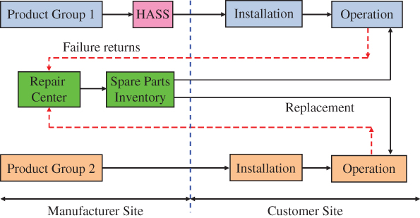
Figure 5.15HASS versus non‐HASS product flow.
where {λ1, β1}, and {λ2, β2} are the model parameters corresponding to two groups, respectively. Based on the respective failure intensity rates of product groups with and without HASS, the rate difference is obtained as follows:
Considering that HASS eliminates infant mortality, we would expect the difference between HASSed and non‐HASSed groups to be positive, i.e. Δu(t) > 0 in Eq. (5.7.3).
Table 5.4 Failure intensity of HASSed and non‐HASSed products.
| Time (t) | Single PCB | Group PCB | ||
| HASSed | Non‐HASSED | HASSed | Non‐HASSED | |
| 50 | 0.0153 | 0.0262 | 3.83 | 2.62 |
| 100 | 0.0159 | 0.0301 | 3.97 | 3.01 |
| 200 | 0.0164 | 0.0346 | 4.11 | 3.46 |
| 300 | 0.0168 | 0.0375 | 4.19 | 3.75 |
| 400 | 0.0170 | 0.0398 | 4.25 | 3.98 |
| 500 | 0.0172 | 0.0416 | 4.30 | 4.16 |
| 600 | 0.0173 | 0.0431 | 4.34 | 4.31 |
| 700 | 0.0175 | 0.0445 | 4.37 | 4.45 |
| 800 | 0.0176 | 0.0457 | 4.40 | 4.57 |
| 900 | 0.0177 | 0.0468 | 4.43 | 4.68 |
| 100 | 0.0159 | 0.0301 | 3.97 | 3.01 |
5.7.2 Financial Justification of HASS
In general all business activities are profit‐driven and accordingly implementing HASS is not different from any business decisions. As such it must be financially justifiable from the management team perspective. It is relatively easy to estimate the cost of the HASS process, and the comparisons can be made between HASSed products and non‐HASSed products in terms of cost savings. Assumptions for developing the financial model are made as follows:
- HASS will eliminate infant mortality by identifying and remedying the causes for early failures due to design weakness, quality defects, and process issues. See Silverman (2000) and Doganaksoy (2001).
- Field failure data and repair analysis reports are used to revise the product design and manufacturing processes to iron out all causes for no fault found (NFF) failures (Janamanchi and Jin 2010). The investigation by Jones and Hayes (2001) indicates that the complexity of electronic equipment, customer usages, and the operating environment are the potential causes for NFF, yet none of them can be effectively eliminated by HASS.
- Products with or without HASS are manufactured using the continually improving and evolving product design and production processes. This assumption actually occurs in the manufacturing industries where information systems such as the Failure Reports and Corrective Actions System (FRACAS) are employed to systematically track failure modes, identify critical issues, and allocate resources to improve the reliability of field products.
There are four major cost items associated with HASS implementation: labor, material, facility, and opportunity costs. Material costs refer to the consumables (e.g. liquid nitrogen, electricity), replacement components, and other incidental materials used. Investment in testing beds like environmental chambers and its depreciation (or lease or rentals) are all assumed to be part of the facility costs. Opportunity cost is referred to as the loss of goodwill because a HASS test likely will postpone the product delivery time. Other expenses such as training and documentation costs may also be significant, but for the model simplicity these costs are considered to be insignificant and as such are not included. Therefore, we have
where
- Cl = labor cost per item
- Cm = material cost per item
- Cf = facility cost per item
- Co = opportunity cost per item
The manufacturer incurs the cost of field failures that take place within the warranty period. There are three major cost components of field failures: repair costs (Cr), shipping/logistics costs (Cs), and inventory holding costs (Ch). Repair costs typically consist of material cost, labor cost, and overhead cost at the repair shop. Shipping costs include the delivery of spare parts to the customer sire for replacement and the returning of defective items. Inventory holding costs include the cost of holding the spare parts in the stockroom and the defective items in the repair pipeline. During the time interval [t, t + τ], the cost savings CSAV on account of HASS can be expressed as

where

Notice that k = 1 is for HASSed and k = 2 is for non‐HASSed products. If during the [t, t + τ], τ0 time (τ0 ≤ τ) is used for HASS, then to justify the continuation of HASS, we need the factory repair cost to be higher than HASS costs for the relevant period. By comparing Eqs. (5.7.4) and (5.7.5), we have
It then follows that, if Cf and Cl are incurred more as fixed costs rather than variable costs, then they have to be accounted for accordingly and the use of (τ0 ≤ τ) has no meaning. In other words, idle time of resources set aside for repairing field failures needs to be absorbed in the factory repairs costs. In effect, we would be using τ as a factor instead of τ0 to compute the variable cost component of repairs, while accounting the prorated fixed costs for the relevant period of τ as follows:
5.8 A Case Study for HASS Project
5.8.1 DMAIC in Six Sigma Reliability Program
Company ABC designs and markets high‐end testing equipment for wafer probing and device test in semiconductor manufacturing sector. A system is usually configured with 30–40 PCB modules depending on the functional requirements. While ABC designs the PCB, the manufacturing of these boards are subcontracted to external suppliers. Upon receiving the PCB by ABC's assembly factory, each board undergoes optional testing, system configuration, and system test before customer shipment and installation. If a PCB fails in any one of the in‐house processes, it is returned to the repair shop for root‐cause analysis. When fixed, the board is routed to “Incoming Stock” again. After the system is shipped and installed in the field, the system will be tested for one more time. If a PCB failed in the field test, it is returned to the repair shop. When fixed, it is routed to the “Incoming Stock” as well. The flowchart in Figure 5.16 shows the subcontract manufacturing process, system configuration, in‐house testing, field installation, and final test of new systems.

Figure 5.16Process map from subcontractor, in‐house testing to field installation.
Jin et al. (2011) proposed a closed‐loop HASS program with the objective to implement reliability growth initiatives in a distributed manufacturing and service chain. As shown in Figure 5.17, the proposed program consists of six functional blocks to form a Six Sigma reliability control scheme through DMAIC: Define, Measure, Analyse, Improve, and Control. DMAIC is a data‐driven improvement strategy to optimize and stabilize the business processes of a new product introduction. Tang et al. (2007) emphasize the importance of incorporating operations research and management science techniques for enhancing the effectiveness of DMAIC methodology. It is the core tool to orchestrate and guide Six Sigma projects in manufacturing industries.
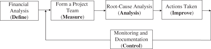
Figure 5.17DMAIC in closed‐loop Six‐Sigma reliability growth (Jin et al. 2011).
5.8.2 Define – Financial Analysis and Project Team
5.8.2.1 Financial Analysis
The Six Sigma program was motivated by customer satisfaction, but the potential cost savings resulted from the improved process is the actual incentive. The resources involved in a repair process include shipping logistics, labor, materials, and testing facilities. To assess the cost benefit of the Six Sigma project, a Monte Carlos simulation program was developed to estimate the cost savings assuming that the infant mortality rate (IMR) could be reduced from the current 14 % to 7% or 3%, and the results are summarized in Table 5.5.
Table 5.5 Potential cost savings of reducing infant mortality rates (IMR) (unit: $).
Source: Reproduced with permission of Elsevier.
| Target rate | Time (month) | T = 3 | T = 6 | T = 9 | T = 12 |
| IMRa = 7% | Average | 358 209 | 716 613 | 1 074 189 | 1 429 820 |
| Standard deviation | 63 692 | 90 500 | 110 737 | 129 480 | |
| Optimistic | 462 972 | 865 473 | 1 256 336 | 1 642 796 | |
| Pessimistic | 253 445 | 567 754 | 892 043 | 1 216 845 | |
| IMRa = 3% | Average | 564 734 | 1 128 324 | 1 696 137 | 2 259 437 |
| Standard deviation | 102 049 | 147 199 | 180 477 | 206 932 | |
| Optimistic | 732 590 | 1 370 445 | 1 992 996 | 2 599 810 | |
| Pessimistic | 396 878 | 886 202 | 1 399 278 | 1 919 064 |
For example, if IMR is down to 7%, the average saving over three months would be $358 209, and $1 429 820 over 12 months. The simulation data allows us to estimate the mean and standard deviation of the savings. At 90% confidence level, the optimistic savings (OSs) and the pessimistic savings (PSs) over the three‐month period are given as
The upper and lower cost savings are very important because they comprehend the uncertainties of the SixSigma program in actual implementations. Similar interpretations can be applied to the potential cost savings under IMRa = 3%.
5.8.2.2 Forming a Cross‐Functional Team
Effective implementation of Six‐Sigma programs requires the formation of a cross‐functional team spanning engineering, operations, supply, marketing, and field services. Figure 5.18 shows the hierarchical structure in which members from different departments are selected both vertically and horizontally to form the Six‐Sigma team. For example, the members from engineering are responsible for eliminating design weakness, correcting software bugs, and updating the software versions. Operations engineers are responsible for manufacturing, handling, and installation issues. Elimination of NFF failures is challenging because various reasons cause NFF returns. One approach is that field engineers work closely with the customer to collect the onsite failure signature, and then send it to the repair center along with the defective part. Finally, the market engineer is able to design the financial metrics to gauge the cost benefit based on the savings upon the implementation of the Six‐Sigma program.

Figure 5.18Formation of a cross‐functional team.
5.8.3 Measure – Infant Mortality Distribution
Based on the system installation dates and the defective PCB return time, Pareto charts are generated to visualize the early PCB failures, and the results are shown in Figure 5.19. The Pareto chart shows that among all the failures, 34% occurred within 30 days of installation, and 18% of the failures occurred within 10 days of installation. The failure trend strongly supports the hypothesis that the current PCB manufacturing and testing process needs to be re‐examined so as to reduce the IMR.
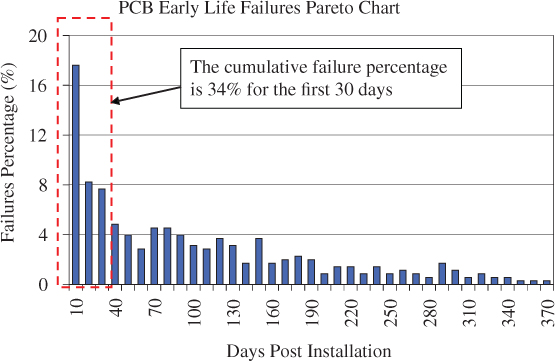
Figure 5.19PCB infant mortality distribution.
Source: Reproduced with permission of Elsevier.
5.8.4 Analyze – Root Cause of Early Failures
In this phase, the team's objective is to concentrate on the process map and narrow the process input variables down to the vital few variables, because they have the greatest impact on the early failure rate. Two hypotheses are created as the objective for the controlled experiment:
- Determine whether PCB is undergoing a thermal/vibration screening or HASS outperforms the PCB that have not.
- Determine whether PCB is undergoing multiple power cycling tests or outperforms PCB that have not.
Two controlled batches of PCB with 100 each were used in the controlled experiment. The first batch of PCB underwent the thermal/vibration screening and power cycling before they were delivered to the system configuration. The second batch of PCB, after being received from subcontract manufacturers, go directly into the system integration without going through HASS and power cycling tests. To minimize the customer usage effects, these boards were mixed randomly and configured into new systems being shipped to different customers. The reliability of these PCB can be easily tracked by the board's unique series number.
After the 30‐day field operation, failure reports of both batches revealed that there were eleven failures among 100 non‐HASS and non‐Power Cycle boards (11%). Only three failures were observed from 100 HASSed and Power Cycled boards (3%). A two‐proportion hypothesis test (Gupta 2004) was performed comparing the two batches of PCB populations. The hypothesis of the test is given below:
The test statistics are

Here p1 and p2 represents the failure rate for both batches, respectively. In addition, ![]() and
and ![]() are the corresponding estimates. In our example, x1 = 11, x2 = 3, n1 = n2 = 100. The two‐proportion hypothesis test revealed that we could conclude with 98% confidence that the HASSed and Power Cycled Tested population performed much better than those without HASS and Power Cycled during the first 30‐day operational period.
are the corresponding estimates. In our example, x1 = 11, x2 = 3, n1 = n2 = 100. The two‐proportion hypothesis test revealed that we could conclude with 98% confidence that the HASSed and Power Cycled Tested population performed much better than those without HASS and Power Cycled during the first 30‐day operational period.
5.8.5 Improve – Action Taken
Based on the result of hypothesis test, the recommendations were given by the team to implement a one‐day HASS process followed by automated power cycling tests in subcontract manufacturers. Specifically, the improvement plan highlights the following action items:
- Establish an ad‐hoc team consisting of mangers and engineers between the host company and each subcontract manufacturer to standardize the improvement process. Agreement should be reached among cost sharing and benefits resulting from the new process.
- Implement HASS and power cycling tests in all subcontract manufacturers within three to five weeks.
- Develop an automated database visible to relevant managers and engineers of the host company and the subtract manufacturers to track the implementation progress.
5.8.6 Control – Monitoring and Documentation
A control plan is developed to monitor and respond to any issues arising from the key inputs and outputs of the new process. The plan included two core components:
- Process Implementation Qualification Report (PIQR) – This report is used to evaluate the HASS and Power Cycling tests conducted by the subcontract manufacturers. The report documents the physical observations and quantitative data related to the process inputs and outputs. If variations arise from the process, the team will take corrective actions along with the subcontract manufacturers.
- Generate and update a statistical process control (SPC) chart for the PCB IMRs – The purpose of the SPC chart is to monitor the reliability performance of the PCB coming from the subcontract manufacturers in a time sequence. The SPC chart in Figure 5.20 shows that the IMR is reduced from 14% to 6.9% in week 40, and remains at the low level thereafter showing the effectiveness of the DMAIC procedure.
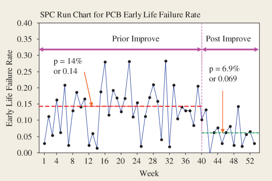
Figure 5.20Tracking the infant mortality rate.
Source: Reproduced with permission of Elsevier.
References
- Arrhenius, S.A. (1889). Über die dissociationswärme und den einfluß der temperatur auf den dissociationsgrad der elektrolyte. Zeitschrift Für Physikalische Chemie 4: 96–116. doi: 10.1515/zpch‐1889‐0108.
- Bennett, S. (1983). Log‐logistic regression models for survival data. Applied Statistics 32 (2): 165–171.
- Boccaletti, G., Borri, F.R., D'Esponosa, F., and Ghio, E. (1989). Accelerated tests. In: Microelectronic Reliability II. Integrity Assessment and Assurance (ed. E. Pollino). Chapter 11. Norwood, MA: Artech House.
- Cox, D.R. (1972). Regression models and life tables (with discussion). Journal of the Royal Statistical Society, Series B 34: 187–220.
- Doganaksoy, N. (2001). HALT, HASS and HASA explained: accelerated reliability techniques by Harry McLean. Technometrics 43 (4): 489–490.
- Elsayed, E. (2012). Reliability Engineering, Chapter 6, 2e. Hoboken, NJ: Wiley.
- Elsayed, E. and Chan, C.K. (1990). Estimation of thin‐oxide reliability usin g proportional hazards model. IEEE Transactions on Reliability 39 (3): 329–335.
- Elsayed, E. and Jiao, L. (2002). Optimal design of proportional hazards based accelerated life testing plan. International Journal of Materials and Product Technology 17 (5/6): 411–424.
- Escobar, L.A. and Meeker, W.Q. (2006). A review of accelerated test model. Statistical Science 21 (4): 552–577.
- Gorjian, N., Ma, L., Mittinty, M., Yarlagadda, P., Sun, Y., (2009), “A review on reliability models with covariates,” in Proceedings of the 4th World Congress on Engineering Asset Management, Athens, Greece, pp. 1–6.
- Gupta, P. (2004). The Six Sigma Performance Handbook: A Statistical Guide to Optimizing Results, 1e. McGraw‐Hill.
- Janamanchi, B. and Jin, T. (2010). Reliability growth vs. HASS cost for product manufacturing with fast‐to‐market requirement. International Journal of Productivity and Quality Management 5 (2): 152–170.
- Jardine, A.K.S., Anderson, P.M., and Mann, D.S. (1987). Application of the Weibull proportional hazards model to aircraft and marine engine failure data. Quality and Reliability Engineering International 3 (2): 77–82.
- Jin, T., Janamanchi, B., and Feng, Q. (2011). Reliability deployment in distributed manufacturing chain via closed‐loop six sigma methodology. International Journal of Production Economics 130 (1): 96–103.
- Johnston, D.R., LaForte, J.T., Podhorez, P.E., and Galpern, H.N. (1979). Frequency acceleration of voltage endurance. IEEE Transactions on Electrical Insulation 14 (3): 121–126.
- Jones, J. and Hayes, J. (2001). Investigation of the occurrence of: no‐faults‐found in electronic equipment. IEEE Transactions on Reliability 50 (3): 289–292.
- Klinger, D. J. (1991a). “On the notion of activation energy in reliability: Arrhenius, Eyring and thermodynamics,” in Proceedings of Annual Reliability and Maintainability Symposium, New York, NY, pp. 295–300.
- Klinger, D.J. (1991b). Humidity acceleration factor for plastic packaged electronic devices. Quality and Reliability Engineering International 7 (5): 365–370.
- Kobbacy, K.A.H., Fawzi, B.B., Percy, D.F., and Ascher, H.E. (1997). A full history proportional hazards model for preventive maintenance scheduling. Quality and Reliability Engineering International 13 (4): 187–198.
- Liao, H., Zhao, W., Guo, H., (2006), “Predicting remaining useful life of an individual unit using proportional hazards model and logistic regression model,” in Proceedings of Annual Reliability and Maintainability Symposium, pp. 127–132.
- Mann, N.R., Schafer, R.E., and Singpurwalla, N.D. (1974). Methods for Statistical Analysis of Reliability and Life Data. New York, NY: Wiley.
- McCullagh, P. (1980). Regression models for ordinal data. Journal of the Royal Statistical Society, Series B 42 (2): 109–142.
- Miller, R. and Nelson, W. (1983). Optimum simple step‐stress plans for accelerated life testing. IEEE Transactions on Reliability R‐32 (1): 59–65.
- Nelson, W. (1990). Accelerated Testing Statistical Models: Test Plans and Data Analyses. New York, NY: Wiley.
- NIST (National Institute of Standards and Technology), Engineering Statistics Handbook, Chapter 8. Available at: http://www.itl.nist.gov/div898/handbook/apr/section1/apr152.htm (accessed on September 2017)
- O'Quigley, J. (2008). Proportional Hazard Regression. New York, NY: Springer.
- Pakbaznia, E., Pedram, M., (2009), “Minimizing data center cooling and server power costs,” In ISLPED'09 Proceedings of the 2009 ACM/IEEE International Symposium on Low Power Electronics and Design, pp. 145–150, San Fancisco, CA, August 19–21, 2009.
- Silverman, M. (2000), “HASS development method: screen development, change schedule, and re‐prove schedule,” in Proceedings of the Annual Reliability and Maintainability Symposium, pp. 245–247.
- Tang, L.C., Goh, T.N., Lam, S.W., and Zhang, C.W. (2007). Fortification of Six Sigma: expanding the DMAIC toolset. Quality and Reliability Engineering International 23 (1): 3–18.
- Wang, W. and Kececioglu, D.B. (2000). Fitting the Weibull log‐linear model to accelerated life‐test data. IEEE Transactions on Reliability 49 (2): 217–223.
- Yan, L. and English, J.R. (1997). Economic cost modeling of environmental‐stress‐screening and burn‐in. IEEE Transactions on Reliability 46 (2): 275–282.
- Yang, G. (2007). Life Cycle Reliability Engineering, Chapter 7, 1e. Hoboken, NY: Wiley.
- Yang, G.B. (1994). Optimum constant‐stress accelerated life‐test plans. IEEE Transactions on Reliability 43 (4): 575–581.
- Yang, K. and Yang, G. (1999). Robust reliability design using environmental stress testing. Quality and Reliability Engineering International 14 (6): 409–416.
- Ye, Z.‐S., Murthy, D.N.P., Xie, M., and Tang, L.‐C. (2013). Optimal burn‐in for repairable products sold with a two‐dimensional warranty. IIE Transactions 45 (2): 164–176.
- Zhao, X. and Xie, M. (2017). Using accelerated life tests data to predict warranty cost under imperfect repair. Computers and Industrial Engineering 107 (5): 223–234.
Problems
State the difference between testing specifications of HALT and HASS.
- List the common stresses that are used in HALT or HASS tests.
- Across the product lifecycle, which ones are subject to HAL and HASS tests: early design and prototype, new product introduction period, volume production, and end of product life.
- Is ESS a type of HASS test? What are the main differences between ESS and HASS?
- Burn‐in, thermal cycling, thermal shock, power cycling, and voltage margining all belong to the HASS process. Give one application (i.e. example) for each test where they are used in product development or manufacturing.
- The following stress profiles are commonly applied: sinusoid, step‐stress, dwell and ramp‐up, and cyclic stress. If the stress types are temperature, please explain which of these stress profiles are more applicable to temperature in reality? What about other stress types like vibration, voltage, power cycling, and force?
- Plot the PDF of a lognormal distribution at Af = 10 and 100 given μn = 10 and σn = 3.
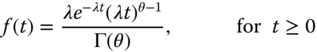
- The failure time of the FPGA (field programmable gate array) follows the gamma distribution and the PDF is given by
where λ is the scale parameter and θ is the shape parameter. Assuming that the FPGA is subject to the HALT test and the relation between the normal and stressed levels are governed by E[Tn] = AfE[Ts], where Tn and Ts are the normal and stressed life and Af (for Af > 1) is the acceleration factor, do the following:
- Let λs be the scale parameter at the stress level. Estimate λn, the scale parameter at the normal condition, assuming that θ remains constant.
- Find the hazard rate function in the normal condition.
- Given λs = 0.01 failure/hour, θ = 2.5, and Af = 200. If the FPGA has tested for 20 hours at the stressed level, what is its equivalent operating hours at the normal condition?
- The lifetime of a bearing can be modeled as a two‐parameter Weibull distribution {θ, β}. The bearing is tested under an accelerated stress condition by applying accelerated forces and vibration stresses, and the reliability reaches 0.65 after 100 000 rotations. Assuming that θn = 4.5θs, where θn and θs are the scale parameters in the normal and stressed conditions, respectively, do the following, assuming that β = 3.2 does not change under the stress:
- (1) Estimate the PDF of the bearing life under normal operating conditions.
- (2) What is the reliability upon 100 000 cycles in normal use?
- (3) Estimate the acceleration factor.
- Reliability of electronics devices are sensitive to their operating temperature. Under the normal operating temperature of 30 °C, the mean‐time‐to‐failure (MTTF) of a microprocessor is 10 years and the standard deviation is three years. The manufacturer wants to design a HALT test to verify this MTTF value. It is known that the relation between the acceleration factor and temperature is as follows:

where Ts and Tn are the temperature at the stressed and normal conditions, respectively. Do the following:
- If the HALT test must be completed in 30 days, what is the minimum temperature stress applied?
- If the device lifetime follows the lognormal distribution, find the PDF under the normal condition and the stressed condition, respectively.
- If the customer requires that the device must survive for 15 years at 90% confidence, determine the highest operating temperature under which this device can run.
- Briefly describe the three most common causes of strength degradation of mechanical components. Give an example of each and also provide methods to prevent or reduce the chance of failures.
- Miner's law is used to predict the expected time‐to‐failure of mechanical components in fatigue. A component was tested under three stress levels and their mean cycles to failure are listed in the table below. Do the following:
Stress level (×106 N/m2) 6.5 8 10 Mean cycles to failure (×105) 13 11.5 7.4 - (1) The proportion of using these stress level in the field would be 0.7, 0.2, and 0.1, respectively. What is the equivalent life of the component?
- (2) Can you estimate the mean cycles to failure under the stress level of 7 × 10⁶ N/m2?
- (3) If the component operates at a single stress level and the measured cycles to failure is 9.5 × 10⁵, what is the stress level?
- Suppose an electronic device operating at T = 40 °C continuously for tf = 2.5 years prior to its failure. Based on the Arrhenius law, estimate Ea of this device assuming A = 0.1 hour.
- For the Arrhenius model, plot the relation between time‐to‐failure and activation energy at T = 25 °C and 50 °C, respectively, assuming A = 0.01.
- A two‐stress Eyring model involves temperature T and voltage V. Assuming Ea = 0.4 eV, B = 1, and C = 1,do the following:
- (1) Plot the relationship between the mean lifetime and T for given A = 0.1, m = 0.3 and S = 10 V and 15 V.
- (2) Plot the relationship between the mean lifetime and S (voltage) for given A = 0.1, m = 0.3 and T = 25 °C and 70 °C.
- (3) Since there is no interaction between T and S, the Eyring model in Eq. (5.5.1) can be expressed as

Re‐plot subproblems (1) and (2) in logarithmic scale.
- Consider the following times‐to‐failure data at two different stress levels.
Stress (V) Times to failure 20 11.1, 16.3, 18.5, 24.1 36 2.2, 3.1 3.6, 4.7, 4.9, 5.8, 6.1, 6.8, 7.4, 8.2, 9.1, 10.4, 10.7, 12.2 14.3, 15.2 Using the maximum likelihood function, use the Weibull inverse power law to model the parameter (also see http://reliawiki.com/index.php/Inverse_Power_Law_Relationship).
- The PHM belongs to the statistics‐based (or non‐parametric) HAT model. Describe the concept of the PHM. State two major differences between the statistical HAL model and physical‐experimental based models, such as the Arrhenius and Eyring models.
- In an accelerated life test, 20 devices are placed in an environmental chamber for constant temperature stressing at T1 = 150 °C. Two devices failed at t = 900 and 960 hours, and the test is terminated at t = 1000 hours with 18 devices surviving. Another test is performed on 4 devices under a higher temperature of T2 = 310 °C. Three devices failed at t = 450, 630, and 850 hours. The last device is removed from the test at t = 700 hours. Do the following:
- (1) Define the covariate of this HAL test and present the PHM.
- (2) Formulate the partial likelihood function and solve for the coefficients of corresponding covariates.
- (3) Assuming the Weibull baseline hazard rate function with θo = 1200 and β = 3.5 and estimate the hazard rate function at T1 = 150 °C and T2 = 310 °C, respectively.
- (4) What is the hazard rate function at temperature T = 200 °C?
- A group of 20 products spend between 0 and 2.75 days in HASS. Note that “0” means the product failed in three months of field use and “1” means passes through three months. How does the number of hours affect the probability that the product will survive the field during the first three months? Use the logistics regression model to solve this.
The table shows the reliability data of 20 samples in the first three‐month field operation.
Days 0.5 0.75 1 1.25 1.5 1.75 1.75 2 2.25 2.5 0.5 Pass 0 0 0 0 0 0 1 0 1 0 0 Days 2.75 3 3.25 3.5 4 4.25 4.5 4.75 5 5.5 2.75 Pass 1 0 1 0 1 1 1 1 1 1 1 - Two batches of PCB modules will be shipped and installed in the field. The size of the batches are n1 = 30 and n2 = 20 and group 1 products undergo HASS and group 2 do not. The table below lists the field returns of failures after one year installation. Note that hours represent the cumulative operating time of that returned item.
Three HASSed products: 1050, 3700, 7900
Seven non‐HASSed products: 330, 540, 890, 1200, 3400, 5700, 8200
Do the following:
- (1) Estimate {λ1, β1}, and {λ2, β2} for both product groups using the Crow/AMSS model.
- (2) What is the intensity difference between two groups at t = 100, 200, and 300 days?
- (3) How many failures would be expected from both groups within a year if n1 = n2 = 100?
- Two batches of products are installed in the field. One is subject to HASS and the other is not. Each batch has 20 items. The failure intensity post HASS is λ1 = 0.001 failures/hour and β1 = 1.1. The item without HASS is λ2 = 0.0012 failures/hour and β2 = 1.3. The costs associated with HASS are Cl = $250/item, Cm = $220/item, Cf = $350/item, and Co = $7000. The costs for repairing a failed item are Cr = $370/item, Cs = $260/item, and Ch = $250/item. Assuming that the HASS implemented at t = 0, estimate the breakeven point of τ such that HASS is more economical than non‐HASSed products.