
4
Determinants of Real Exchange Rate in Papua New Guinea
4.1 Introduction
As discussed in Chapter 2, the real exchange rate - the price ratio of tradable to nontradable goods - is the key link between resources booms and their impact on the performance of an economy. Like other relative prices, real exchange rates are affected by real and nominal disturbances, which may be either long lasting or transient. A real exchange rate reacts to a series of real and nominal disturbances, including international terms of trade (TOT) shocks, government expenditure patterns, trade restrictions, net capital inflow and technological progress, as well as to domestic credit creation and nominal devaluation.
The objective of this chapter is twofold: to construct a real exchange rate index and to identify the major determinants of real exchange rate behaviour using a dynamic model of real exchange rate determination. Section 4.2 of this chapter presents the general concept of the real exchange rate; Section 4.3 constructs several series of real exchange rates for PNG, discusses the problems of constructing such indices, and offers alternative measures to overcome the problems; Section 4 develops a dynamic model of real exchange rate determination to analyse how the long-term equilibrium real exchange rate reacts to a series of real disturbances, and also attempts to develop a monetary model incorporating variables determining the movements of the actual real exchange rate; Section 4.5 presents an empirical model of the real exchange rate using the theoretical model developed in Section 4.4; Section 4.6 presents the data sources and the different measures of variables employed; Section 4.7 shows the econometric procedures used; Section 4.8 presents the empirical results; and Section 4.9 summarises conclusions.
4.2 Concept of Real Exchange Rate
The real exchange rate (RER) can be defined as the ratio of relative price of tradables (PT) with respect to nontradables (PNT). This ratio, which is also known as the ‘Salter ratio’, can be written symbolically as follows:
It is clear from the above definition that real exchange rate is a concept that measures the relative price of two goods as opposed to the nominal exchange rate, which is a measure of two monies (Edwards, 1988b). International competitiveness is usually measured in terms of real exchange rate movements. The definition of RER focuses on the rate at which tradables are exchanged for nontradables, or the cost of domestically produced tradables (Edwards, 1988b). A fall in this ratio represents an appreciation of RER, induced by an increase in the price of nontradable goods, and/or by a reduction in the relative price of tradables to nontradables. Real exchange rate appreciation is synonymous with a deterioration in a country’s international competitiveness, as it increases the profitability of the nontraded sector and attracts resources from other traded sectors, as well as increasing the domestic cost of producing tradable goods. By contrast, an increase in this ratio represents a real depreciation, or an improvement in the international competitiveness of tradable production.
It is important to recognise a fundamental notion about the concept of RER. RER is not unique for every sector of an economy. Within the tradable sectors, different real exchange rates can be observed for import substitutes and for exportables. For example, an exporter’s real exchange rate can be significantly different from the real exchange rate for an importer, due to costs and productivity differences in these sectors. For these reasons different RER indices are used separately to identify the changes in the competitiveness of importable and exportable sectors of an economy.
4.3 Real Exchange Rate Indices
Construction of a RER index is difficult, since the exact counterpart of the price of tradables (PT) and nontradables (PNT) is not directly observable. Furthermore, in the presence of quantitative trade restrictions, some potentially tradable sectors behave as nontradable sectors. Thus, disaggregation between these sectors becomes less meaningful. Empirical study to examine the theory of the real exchange rate in the tradable and nontradable spheres has always lagged behind due to the limitations of precise variable measurement and difficulty in obtaining data along tradable and nontradable lines.
Disaggregating GDP between the tradable and nontradable sectors and deriving the price ratio of these two sectors to observe RER movements can construct the most direct measure of the RER. GDP and imports of goods and services are divided into two broad divisions of tradables and nontradables. Tradable goods are defined as goods and services that are either traded internationally or could be traded at some ‘plausible range of variation in the relative prices’ (Goldstein and Officer, 1979, p. 415). Therefore, tradable goods have a wider scope than traded goods and their prices are determined by world prices and exchange rates. Nontradables are those goods and services that, for reasons (such as transport costs) cannot be traded internationally. Their prices are determined by the interaction of domestic demand and supply conditions. Goldstein and Officer (1979) suggest three criteria to draw the distinction between tradable and nontradable goods. First, tradable goods have a higher degree of foreign trade participation rate than nontradables. Secondly, correlations of price changes for tradables are much higher across countries than for nontradables, and finally, tradables are closer substitutes for traded goods than are nontradables.
The method of disaggregating GDP into tradable and nontradable sectors has two fundamental drawbacks. First, in most developing countries this disaggregation of GDP between tradables and nontradables is too broad to compare across sectors. Second, in the presence of quantitative trade restrictions, some tradable sectors behave as nontradable sectors and, in this case, the existing disaggregation between tradable and nontradable sectors does not provide a meaningful comparison.
A more practical proposition is to construct the real exchange rate index by disaggregating the components of the CPI into tradable and nontradable categories. Housing, rent and power components of domestic CPI can be commonly used as proxies for nontradable prices.1 This method also has some drawbacks, because, although this price index of nontradables includes most of the nontradable elements, it also incorporates some tradable items such as fuel and household equipment in production. Another problem with this index is in selecting appropriate weights to be attached to each component of this proxy. Furthermore, with very few exceptions, disaggregated CPI data are not readily available on an annual basis in most developing countries, including PNG.
Given the practical limitations of direct measures, RER is usually proxied by the following measure:
where e is the nominal exchange rate defined as a domestic currency price of foreign currency, PT* is the foreign price, and P is the domestic price level. The PT is a composite price measure of exportables and importables and the domestic price level, P, measures the domestic price of nontradables (PNT). Therefore, the real exchange rate is the ratio of foreign prices measured in domestic currency to the domestic price level.
The problem with constructing the above index starts with the choice of an appropriate nominal exchange rate. Should the nominal exchange rate be with respect to a single foreign currency, that is, a bilateral exchange rate, or does the nominal exchange rate have to be a weighted average of bilateral exchange rates of major trading partners? Then comes the problem of choice of weights. Traditionally trade weights are popularly used to capture the trading pattern of a country. Corden (1984) conjectures whether services and remittances should be included alongside the merchandise trade weights. The problem is further complicated by the existence of multiple exchange rates systems in some developing countries.
Several alternative price indices for the PT and PNT have been suggested as possible candidates for the construction of a PPP-based RER. The popular and common practice is to construct a real exchange index by deflating the trade-weighted nominal exchange rate adjusted for foreign price by a proxy for domestic nontradable price. The most widely used proxy for tradable and nontradable price is CPI. This measure is popular, since almost every country publishes CPI on a regular basis.
But the foreign CPI index has a major drawback as a fair proxy for the PT. The deficiency of using this index is that CPIs include large elements of nontradable prices. If, for example, the price of foreign nontradables increases relative to the price of tradables, then this increase in the PNT will reflect on the foreign CPI. Therefore, foreign CPI, as a proxy for tradable prices, is not appropriate as it may overstate the relevant foreign inflation and thereby overstate the depreciation of the real exchange rate (Little et al., 1993, p. 259).
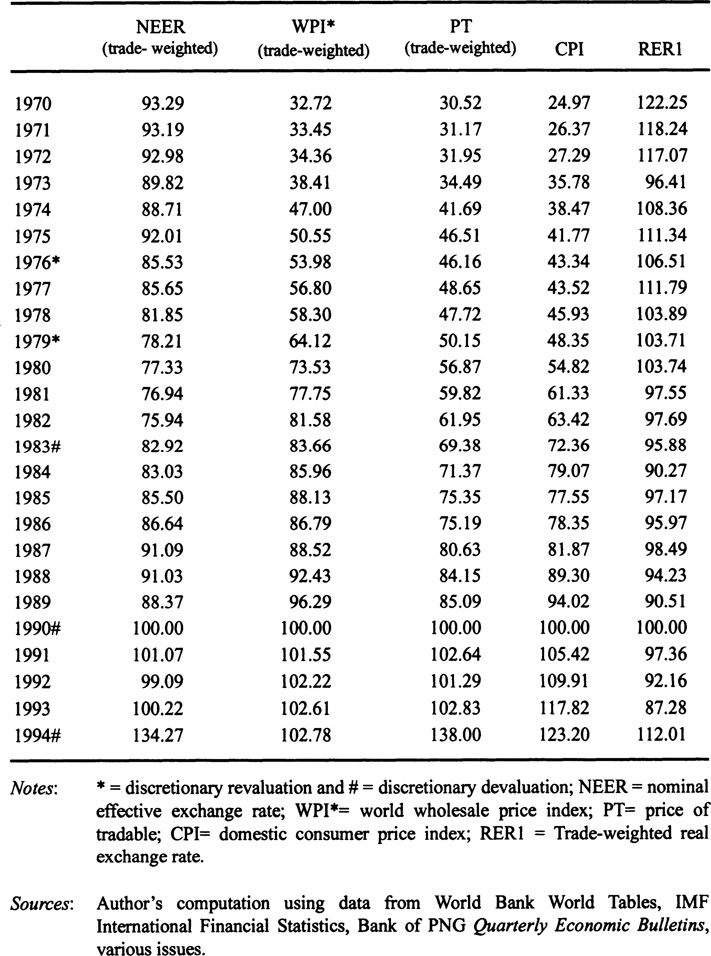
Because of the problem associated with the use of CPI as a proxy for the PT, the use of the foreign wholesale price index as a proxy of PT to measure the RER is the most common practice. We used this measure of trade-weighted real exchange rate (RER1) for our study. Therefore, the trade-weighted real exchange rate is defined as:
where WPI* is the foreign wholesale price index proxied for the world price of tradables, eTW is the trade-weighted nominal effective exchange rate and P is the domestic price level representing the price of domestic nontradables. Using average trade-weighted WPI*s as proxy for tradables solves some of the problems arising from using foreign CPIs. WPI* is heavily weighted with tradable items and does not include services. There may arise some possibility of double counting while using WPI as a proxy for the price of tradable, since WPI measures commodity prices at varying stages of production. Despite this minor limitation, WPI is considered to be the most reasonable proxy for the world price of tradables.
Domestic CPI is the standard proxy for the PNT since the major components of the domestic CPI basket comprises nontradable goods and services. The price deflator for GDP is another common proxy that is used for the PNT. Neither CPI nor the GDP deflators are appropriate indicators of the price of nontradables, since both of these indices measure the price movement as an aggregate of tradable and nontradable goods and services and do not just represent independently the separate price movement for nontradables. The GDP deflator has one advantage over the CPI index as it captures all domestic price movements on a value added basis (Goldstein and Officer, 1979). To overcome the limitations of CPI and GDP deflators as a proxy for the PNT, some authors disaggregate the CPI components into tradable and nontradable goods and services and then take the weighted average of the nontradable components of CPI to construct a price index for nontradables. This index, represents the proper price movements for nontradables, and is the most appropriate method if data is available.
So far, the PT has been considered as a composite price of importables and exportables as in Salter’s (1959) dependent economy model. But a distinction between the price of importables and the price of exportables is necessary as different trade controls and changes in international prices can affect the price movements in exportables and importables quite differently. Moreover, domestic quantitative trade restrictions can affect the price of importables more than exportables and may change some import substitutes into nontradable categories. Therefore, it has been argued that it is more appropriate to use the export price index (EPI) and import price index (IPI) separately as proxies for the world price of exportables and importables. This division of EPI and IPI clearly reflects the price movements of goods and services that are actually traded.
Therefore, two other commonly used direct measures of the real exchange rate can be defined as the relative price of exportables to nontradables (proxied either by the domestic CPI or GDP deflator or by the weighted average of nontradable components of CPI):
and the relative price of importables to domestic nontradables,
which can serve as direct measures of competitiveness in the tradable sectors of an economy. But the use of these indices to proxy the world price of tradables has also faced some criticism. It is argued that these indices (EPI, IPI) have well known deficiencies as measures of price of heterogeneous commodity groups and are generally expressed in unit value terms. It is, therefore, not surprising that there exists quite a number of different measures of the real exchange rate, given that there could be several possible proxies used to represent the PT and nontradables.
The next sub-section attempts to construct the three indices - RER1, RER2, RER3 -for PNG
4.3.1 Real Exchange Rate Indices for Papua New Guinea
Three alternative measures of real exchange rates have been constructed namely RER1, RER2 and RER3. RER1 is reported in Tables 4.1. In Table 4.1 the trade- weighted nominal effective exchange rate (NEER) of PNG has been multiplied by the weighted average of the wholesale price indices of PNG’s major trading partners (Australia, Japan, UK, US and West Germany). As discussed earlier, this measure represents the index of trade-weighted world price of tradables (PT-trade) converted in terms of PNG’s domestic currency (kina) value. With respect to the domestic price of nontradables, PNG’s consumer price index has been used as an approximate measure of the PNT. The world price of tradables is then deflated by the domestic CPI to construct the index of the trade-weighted real exchange rate (RER1) for PNG. Trade shares2 of major trading partners in 1990 have been used as weights in the calculation.
Some substantial exchange rate movements, as reflected in the trade-weighted NEER, resulted from discretionary exchange rate policy measures.
The NEER index for PNG indicates a significant appreciating trend in the post-independence period between 1975 and 1982. This nominal appreciation reflects PNG’s ‘hard kina’ strategy to insulate the domestic economy from imported inflation by revaluation of the kina several times after monetary independence in 1976. Discretionary depreciations of the kina by 10 per cent in 1983 and 10 per cent in 1990 are reflected in the overall depreciation of the NEER during this period. Then a gradual appreciation from 1991 to 1993 occurred before 1994’s sharp depreciation of the NEER, which mostly resulted from official devaluation of the kina by 12 per cent followed by the subseqcent floating of the kina.
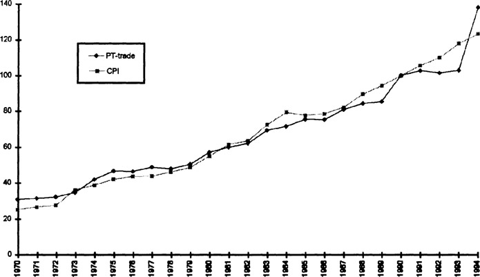
Over the 1970s and the 1980s, the price index of tradables moved very close to the domestic CPI (Figure 4.1). During the 1970s, the PT was on average higher than the price of domestic nontradables. However, the domestic CPI started to rise from the early-1980s and continued until the early-1990s. During this period the change in the PT remained lower than domestic inflation. In 1994, the PT started to rise higher than the domestic price level and to a large extent the economy regained its competitiveness in the world market, as seen in Figure 4.1.
The trend in the real exchange rate of PNG is shown in Figure 4.2. During the construction boom and minerals boom in 1971-73, the domestic wage-price increased faster than the price increase in tradables, which is clearly evident in the real exchange rate appreciation in 1973. The index of RER declined sharply by about 18 per cent in 1973 from the previous year.
The commodity boom of 1976-77 had more moderate effects on real exchange rate movements, due to cautious macroeconomic policies and a gradual reduction in foreign aid flows. Foreign aid fell by about 26 per cent in 1977 from the period of independence (Appendix Table A3.7), which helped to depreciate the RER. This real depreciation in 1977 indicated a ‘reverse resources boom’ in PNG.
WhiletheRERl of PNG appreciated during 1973 because ofrelatively high inflation in PNG compared with its major trading partners, the rate depreciated significantly in 1977, due to virtually imperceptible domestic inflation maintained by prudent macroeconomic policy. A more stable real exchange rate movement from the mid-1970s to the late 1980s was consistent with the objectives of macroeconomic policies intended to control inflation and ensure a stable macroeconomic environment.
Table 4.1 Trade-weighted real exchange rate (RER1) index, 1970–94 (1990 = 100)
The real appreciation from 1990 to 1993 was due to a combination of several external and internal factors. PNG’s inflation rate increased rapidly relative to its major trading partners’ inflation rates during the early-1990s. The resources boom in PNG’s mining sector over this period also impacted upon the PNT, which was fuelled by expansionary fiscal stances. This relative increase in PNT to the PT was quite rapid and appreciated the trade-weighted real exchange rate (RER1) during this period (Table 4.1 and Figure 4.2).
The export price index (EPI) and import price index (IPI) have been deflated by the price index of nontradables (constructed by taking only the weighted average of nontradable items in the CPI basket) to construct the real exchange rates for exportables (RER2) and for importables (RER3) for PNG. These direct measures are reported in Table 4.2 and shown in Figure 4.4. In general, all indices of the real exchange rate (RER1, RER2, RER3) moved quite differently over 1970s. Then the rest of the period they followed a similar pattern (Figure 4.4).
Between 1972 and 1979, the RER2 and RER3 indices show strong depreciation (with an exception in 1975) whereas the trade-weighted real exchange rate (RER1) indicates a significant real appreciation during 1973. RER1 appreciated due to the rate of increase of domestic CPI being higher than the PT, whereas RER2 and RER3 depreciated because export and import price indices were higher than the domestic price of nontradables in the early-1970s (Table 4.2). Over the 1980s, all measures of the RER appreciated on average, due to a declining trend in PNG’s export price index and rapid growth in the domestic price level. After 1992, PNG’s export price index increased significantly and brought about a real depreciation of RER2 over 1993-94 and improved competitiveness for the export sector. But RER1 and RER3 appreciated between 1991-93 before starting to depreciate in 1994, due to flotation and a large depreciation of kina and increase in price of tradables relative to domestic price level (Figure 4.2 and 4.4).

Note: Three different real effective exchange rate indices are constructed by using* import share, export share and trade share as weights. The three measures show a similar pattern in their movements.
Sources: Author’s computation using data from World Bank World Tables, IMF International Financial Statistics, Bank of PNG Quarterly Economic Bulletins, various issues.
Figure 4.2 Real Exchange Rate (RER1) indices of PNG, 1970-94 (1990 = 100)
Now we proceed to develop a theoretical model in order to shed light on the possible determinants of the real exchange rate, which might have impacted upon the movement of PNG’s real exchange rate.
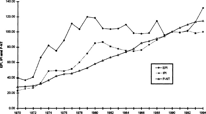
Figure 4.3 Export price index, import price index and price of nontradables(1990 = 100)
Source: Table 4.2
4.4 Theoretical Framework
The basic theoretical framework used in this study has been adopted from Edwards’ (1989) model of real exchange rate determination. The model captures most of the stylised features of a small open developing economy, including the existence of exchange and trade controls. This model allows only the ‘fundamentals’ or real variables to play a role in determining the long-term equilibrium real exchange rate, whereas both real and nominal factors influence the actual real exchange rate in the short term.
The model assumes a small, open economy, which produces and consumes two goods - tradables and nontradables. Importables and exportables are aggregated into one tradable category. The government sector consumes both tradables and nontradables and finances its expenditures by non-distortionary taxes and domestic credit creation. The country holds both domestic money and foreign money. At a later stage of the study it is assumed that there are no capital controls, and that there are some capital flows in and out of the country. The nominal exchange rate of the economy is fixed with a basket of currencies of its major trading partners. It is also assumed that there is a tariff on imports. The price of tradables in terms of foreign currency is fixed and equal to unity that is, PT = 1. Finally perfect foresight is assumed in this model.
Table 4.2
Real exchange rate indices for export and import competing sector (1990 = 100)
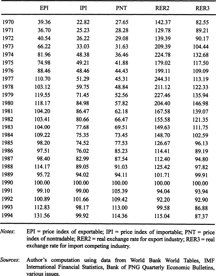
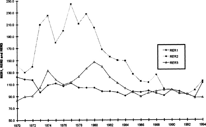
Figure 4.4 Real exchange rate indices for export and import competing sectors, 1970-94 (1990 = 100)
The model is represented by the following equations:
Portfolio Decisions:
| (4.1) |
| (4.2) |
| (4.3) |
Supply Side:
| (4.7) |
| (4.8) |
Government Sector:
| (4.9) |
| (4.9) |
| (4.10) |
| (4.11) |
External Sector:
| (4.12) |
| (4.13) |
| (4.14) |
| (4.15) |
Equation (4.1) defines the total assets, A, as the sum of domestic money M and foreign money FM. Equation (4.2) defines real assets (a) in terms of tradables, where E is the nominal effective exchange rate (foreign currency value in terms of domestic currency). Domestic money (m) and foreign money (fm) are also defined in terms of the nominal exchange rate in this equation. Equation (4.3) shows there is international capital mobility, therefore, FM ≠ 0.
The demand side of the economy is given by equations (4.4) to (4.6). The real exchange rate (e) is defined as the ratio of foreign price in terms of domestic currency to the price of domestic nontradables in equation (4.4). Demand for tradables and nontradables is determined by the real exchange rate and the level of real assets. Asset level positively affects demand for both tradables and nontradables whereas real depreciation reduces the domestic demand for tradables but increases the demand for nontradables, which is shown in equation (4.5) and (4.6).
Equations (4.7) and (4.8) summarise the supply side of the economy. The supply of tradables and nontradables is solely determined by the real exchange rate. An appreciation of the real exchange rate reduces the supply of tradables and increases the supply of nontradables. To keep the model simple the tax function is not included (equations 4.5-4.8) in the demand function and the tariff function is not included in the demand for importables.
Government sector is summarised by equations (4.9) to (4.11), where GNT and GT are government consumption of nontradables and tradables, respectively. Equation (4.9) is the real government consumption of tradables and nontradables in terms of tradable. Equation (4.10) defines the share of government consumption of tradables to the total government expenditure as λ, which is equal to (gT/g) in real terms. Equation (4.11) represents the government budget constraint where government consumption is financed by taxes (t) and domestic credit creation (DC).
The external sector is represented by equations (4.12) to (4.15). Equation (4.12) defines the current account as the difference between the output of tradables and both private and public consumption of tradables expressed in foreign currency. Equation (4.13) indicates that there is inflow and outflow of capital. The capital account is defined as a function of interest rate differentials between domestic and foreign economies. Equation (4.14) defines the change in stock of international reserves. Finally the model is closed with equation (4.15), which shows that the change in domestic money (m) is determined by changes in domestic credit creation and changes in international reserves.
Long-term equilibrium is attained when the nontradable goods market and external sector are simultaneously in equilibrium - which implies that the current account is equal to the capital account in the long term. However, in the short and medium term, there can be departures from CA = K, which will result in the accumulation and decumulation of international reserves. Therefore, the long-term steady state is attained under four scenarios, which can be summarised as follows:
- (1) there is internal equilibrium or equilibrium in the nontradable sector;
- (2) there is external equilibrium so that R = 0 = CA = KA = m;
- (3) the government runs a balanced budget such that G = t and DC = 0, that is, fiscal policy is sustainable; and
- (4) portfolio equilibrium holds.
The real exchange rate attained under these steady-state conditions is known as the long-term equilibrium real exchange rate, ERER, that is,
| (4.16) |
The nontradable market clears when
| (4.17) |
The real government consumption of nontradables in terms of tradables has been defined as gNT. Thus, the PNT can be expressed as a function of a, gNT PT and ſ (trade restrictions).
| (4.18) |
where, δn/δa>0; δn/δgNT>0; δn/δPT>O, δn/δſ>0
Equilibrium in the external sector requires that m = 0. The following equation can be derived from earlier equations as
| (4.19) |
When government expenditures are fully financed with taxes, the R = 0 will coincide with the m = 0.
From (4.18) and (4.19) it is possible to find an equilibrium relation between e, a, gNTand ſ.
| (4.20) |
where δx/δa<0; δx/δgNT<0; δx/δPT>0; δx/δſ<0
An increase in m, domestic money in terms of foreign currency, results in higher real wealth and a current account deficit. To restore equilibrium real wealth, the price of nontradables will rise (4.18). Thus, an increase in the value of real assets increases the price of nontradables and appreciates the RER to maintain long-term equilibrium. Increases in government expenditure on nontradables (gNT) have the same effects on the equilibrium RER. A rise in the PT (through an improvement in TOT due to an increase in the price of exportables) generally depreciates the RER, given that the price of nontradables and the nominal exchange rate remain constant. However, if the increase in the PT increases export earnings, and is spent in the nontradable sector, the demand for and price of nontradables increases more than the PT causing a RER appreciation. The total effect of an import tariff depends on the initial expenditure on domestic nontradables and importables. An increase in the tariff on importables worsens the current account by increasing import bills, lowers the demand for tradables, raises the demand and price for nontradables and tends to appreciate the long-term real exchange rate. But if an increase in tariff worsens the current account balance without any substitution effects, it will increase the composite PT alone and may depreciate the real exchange rate. It is therefore, possible to observe, simultaneously, a real depreciation and a worsening of the current account. So the increase in the PT and changes in trade policies can have either positive or negative impacts on the RER.
Equation (4.20) stipulates that the long-term equilibrium RER is a function of real variables only. The value of real assets, government consumption, price of tradables and trade restrictions in this equation are normally influenced by changes in other real variables such as TOT shocks, changes in government expenditure, technological progress, and changes in trade and capital restrictions. Changes in these real variables can cause the actual RER to deviate from its equilibrium level. However, changes in nominal variables, such as domestic credit expansion, and changes in the values of the nominal exchange rate, also affect the path of the actual RER in the short term. The impacts of real and monetary disturbances on the RER, both in the short- and long-term are discussed in the next section.
4.4.1 Real Disturbances and Misalignment of Real Exchange Rate
Changes in the long-term sustainable values of real variables have important effects on the equilibrium real exchange rate (ERER) and can cause it to deviate from its equilibrium level. This is commonly known as structural misalignment of the real exchange rate. In fact, the movement of the ERER from its sustainable long-term position has significant consequences for policy evaluation as it can imply either gain or loss of external competitiveness. According to the purchasing power parity version of the real exchange rate, this movement of ERER is considered a disequilibrium situation. But according to recent developments in the theory of the real exchange rate this movement of ERER does not necessarily reflect disequilibrium, since the change in ERER is induced by changes in fundamentals, that can represent a new long-term equilibrium for the real exchange rate (Edwards, 1988b). This section attempts to analyse the ways in which the equilibrium RER reacts to a number of real disturbances.
Real exchange rate fundamentals are often categorised as external and domestic fundamentals. Domestic fundamentals can be divided into policy-related and non-policy-related fundamentals. The most important external fundamentals, which affect the RER in the long term, include international terms of trade, and international transfer, including foreign aid and world real interest rates. Included among policy-related domestic fundamentals are import restrictions, export taxes or subsidies, exchange and capital controls, and government consumption expenditure. Technological progress and productivity improvement are the two most important domestic non-policy fundamentals. The role of these fundamental factors is discussed below.
Terms of trade disturbance
International TOT is one of the most important external real exchange rate fundamentals and is often included as one of the major determinants of RER in the literature, since foreign price shocks have accounted for large fluctuations in RERs of both developed and developing countries. The overall effect of TOT on the real exchange rate is ambiguous. The price of tradables is a weighted average of the price of exportables and importables. TOT may have two different effects on the real exchange rate, namely, substitution and income effects. The income effect results when an increase in export prices, or a fall in import prices, raises the income of an economy and increases demand for nontradables. This, in turn, tends to reduce the relative price of tradables to nontradables and so appreciate the RER. On the other hand, the substitution effect can be observed due to relative cheapness of nontradables. Thus an improvement in TOT due to an export price increase brings about a RER depreciation for given levels of nominal exchange rate and nontradable prices. However, if the improvement in TOT is brought about by a fall in the price of imports alone, then the improvement in the current account balance would increase aggregate income and the PNT and cause an appreciation of the RER. The income effect would be more prominent in this case. Because of the ambiguity about the final effects of a TOT shock on the RER, the price of importables and exportables should be regarded as two separate variables in determining real exchange rate behaviour.
Government expenditure
Government expenditure is another fundamental real variable, which can cause the real exchange rate to deviate from its equilibrium value. Increases in government expenditure increase the demand for nontradables if the major portion is spent on nontradable goods and services. In the short term this excess demand for nontradables bids up their price and results in RER appreciation. However, there will be depreciation of the RER if the larger share of government expenditure is spent on the tradable sector rather than on consumption of nontradables. Thus, the sign of this variable can be either positive or negative in determining behaviour of the equilibrium real exchange rate.
Trade restrictions
Trade restrictions in the form of tariff generally cause a RER appreciation. If tariff worsens the current account position and increases the demand for and price of nontradables, the RER appreciates. An increase in binding quantitative trade restriction (import quota) also increases the demand for import substitutes, which behave as nontradables due to imposition of quantitative trade restrictions during a boom period (Warr, 1986). This results in higher prices and profitability for nontradables and leads to a long-term equilibrium real appreciation. In these cases, the increase in the PNT due to trade restrictions is higher than the increase in the composite PT. However, if trade restrictions lead to a worsening of the current account deficit and reduce the demand for nontradables, there will be RER depreciation. In this case negative income effect will overweight the positive substitution effect.
Exchange and capital controls
Relaxation of capital controls may affect the movement of RER in either way. If liberalisation of capital control increases net capital inflow, it leads to expansion in the monetary base. This raises current expenditure over income and increases the demand for nontradables, resulting in an appreciation of the equilibrium RER. A fall in world real interest rates or a rise in international transfers, such as aid flows, also affects the equilibrium RER in a similar way to net capital inflow. If the major share of foreign aid is spent on nontradables, the demand for and price of nontradables increases relative to tradables, which tends to appreciate the RER.
Technological and productivity improvement
The non-policy domestic fundamental variable, namely, technological advancement (growth rate of real GDP), generally increases the efficiency and productivity of the tradable sector. Increased productivity induced by technological progress increases factor availability. By reducing the cost and price of tradables, increased productivity makes the tradable sector more competitive and tends to depreciate the RER of the sector. In this situation, supply effects of technological progress offset the demand effects according to the Rybczynski principle (Edwards, 1989, p. 48). But if the advancement in technology increases income, which, in turn, increases demand for and price of nontradables relative to tradables, there will be a real appreciation. In this case, the demand effects of technological progress are greater than the supply effects and this is known as the Ricardo-Balassa effect (Edwards, 1989, p. 136).
4.4.2 Nominal Determinants and Real Exchange Rate Misalignment
The real exchange rate often departs from its equilibrium values influenced by macroeconomic pressures, which is commonly known as macroeconomic policy induced misalignment of the real exchange rate. The effects of macroeconomic policies and changes in the nominal exchange rate on the real exchange rate will now be discussed.
In order to maintain a sustainable macroeconomic equilibrium in an open economy, fiscal and monetary policies must be consistent with the exchange rate regime. Misalignment of the real exchange rate occurs due to inconsistencies between macroeconomic policies and the official exchange rate policy. Under a fixed exchange rate regime, expansionary monetary or fiscal policy raises the real stock of money, increasing demand for both tradable and nontradable goods and financial assets. The excess demand for tradable goods results in a higher trade deficit and loss of international reserves, whereas the increased demand for nontradables raises their price and tends to deviate the actual RER further from its equilibrium value. The over-valuation of the RER, which is a fall in the actual real exchange rate from its long-run equilibrium, will be short-lived and the economy adjusts through reduction of the money stock. The higher demand for nontradables induced by the higher stock of money, would reqcire a higher (actual) RER to re-establish equilibrium in the nontradables market. The stock of international reserves will fall by the decline of the real domestic money. The actual RER will continuously depreciate through reductions in the price of nontradable goods and revert towards the long-term sustainable equilibrium RER position in the long term.
The time involved in the readjustment of a misaligned RER to its long-run equilibrium depends on the original stock of money as well as a number of other variables. Adjustment of the nominal exchange rate (devaluation/revaluation) could be one possible strategy to speed up this readjustment. In the case of an over-valued real exchange rate, a nominal devaluation reduces the stock of money since m=M/E and thus reduces the real value of financial assets. This induces expenditure reducing effects, by reducing expenditures on both tradable and nontradable goods. A nominal devaluation also induces expenditure-switching effects by reducing expenditure on tradables. It also tends to increase the production of tradables, since the PT is relatively higher and the exportable sector is more competitive following devaluation. This depreciates the RER resulting in an expansion of the export sector. Expenditure switching effects tend to increase the demand for nontradables but expenditure reducing effects may reduce their price. Therefore, following a nominal devaluation, the demand for nontradables increases and the price falls to re-establish equilibrium in the nontradable market, and this induces a real depreciation.
Following a nominal devaluation a number of policies can lead to an increase in the price of nontradables, most obviously expansionary monetary and/or fiscal policy and wage indexation policy. However, if a nominal devaluation is accompanied by restrained fiscal and monetary policies in the absence of wage indexation, the nominal devaluation will probably succeed in generating a real devaluation and achieving competitiveness in the tradable sectors. Simultaneous imposition of an import tariff and an export subsidy can affect the RER in the same way as devaluation. While export subsidies increase demand for and domestic price of exportables, a tariff increases the price of importables, so that the composite price of tradables as a group will increase in this situation. The relative price of exportables and importables will not be affected as long as the rate of tariff and subsidy is the same, but the price of tradables (as a composite measure of exportables and importables) will rise relative to nontradables as in the case of devaluation. However, while devaluation does not affect fiscal policy directly, a tariff with subsidy policy has a direct impact on the government budget. Furthermore, while a tariff with subsidy policy only affects the domestic price of tradable goods and services, devaluation affects the domestic price of both tradable goods and tradable assets. Accordingly, while the expectation of further devaluation may affect the domestic interest rate, the tariff with subsidy policy, does not have any direct effect on the domestic interest rate (Edwards, 1988b, p.31).
4.5 Empirical Model
The purpose of this section is to analyse empirically the relative importance of real and nominal variables in explaining the real exchange rate movements in PNG, as reported in Tables 4.1 and 4.2. In an attempt to estimate the dynamics of the real exchange rate, it is necessary to specify an empirical equation for the equilibrium real exchange rate et*. Based on the theoretical model developed in Section 4.4, the equilibrium real exchange rate is exclusively determined by real variables. According to the discussion in Section 4.4, the most important ‘fundamentals’ in determining the RER are:
- international terms of trade;
- government expenditure;
- trade restrictions;
- exchange and capital controls; and
- technological progress and productivity gain.
Incorporating the above-mentioned ‘fundamentals’ a model of equilibrium real exchange rate was formulated in the following equation.
| (4.21) |
The following notations have been used in the above model:
| et* | : | equilibrium real exchange rate |
| TOT | : | barter terms of trade, defined as Px*/Pm* |
| GEX | : | share of government expenditure to GDP |
| NKI | : | net capital inflow (proxied for capital control) |
| AID | : | foreign aid and grant |
| OP = (X+M)/Y | : | trade restrictions substituted by the openness of an economy3 |
| TECP | : | measure of technological progress |
| ut | : | error term |
The actual RER is a function of both real and nominal variables. Three major factors determine the dynamics of actual RER and are specified by the following equation:
| (4.22) |
where, e is the actual real exchange rate, and e* is the equilibrium RER, which is a function of real variables as specified in equation (4.21). The second determinant of the actual RER in equation (4.22) is MPt, which states that if macro policies were unsustainable in the long term under a fixed rate, there would be a tendency for the RER to appreciate. A large λ represents a large over-valuation of the actual RER from its long-term equilibrium value. Finally, RER movements are affected by the changes in the nominal exchange rate (log Et - log Et-1). A nominal devaluation has a short-term positive impact on an over-valued RER in restoring a misaligned real exchange rate towards its equilibrium value. The actual magnitude of a short-term depreciation of the RER depends on the parameter γ. The long- and medium-term effects of changes in the nominal exchange rate would depend on the initial condition of the equilibrium real exchange rate, log et*, and on the accompanying macroeconomic policies of credit creation. The parameters α, λ, γ are positive and capture the most important dynamic aspects of the adjustment process.
The term, MPt in equation (4.22) indicates the role of macroeconomic policies in determining real exchange rate behaviour. If macro policies were unsustainable in an expansionary direction, the real exchange rate would tend to appreciate, given that the other variables remain constant. To capture the impacts of macro policies, macroeconomic policy behaviour was proxied in two ways. Firstly, by the excess supply of domestic credit, measured as the rate of growth of domestic credit minus the rate of growth of real GDP.
Secondly, the rate of growth of domestic credit is used to measure the macroeconomic policy impacts on real exchange rate movements.
By successive substitution for log et*, the macroeconomic policy variable by excess supply of domestic credit, the rate of growth of domestic credit and the change in nominal devaluation by NDEV in equation (4.22), the following estimable equation for the actual RER is given by:
| (4.23) |
where θs are the combination of αs and βs.
The above model incorporates the real and nominal factors affecting the observed RER both in the short and long term. The “fundamentals” or the real variables affect the equilibrium RER in the long term whereas the nominal variables impacts on the RER only in the short term. An improvement in TOT can result in either real depreciation or real appreciation, and so is the outcome of an increase in government spending. Relaxation in exchange and capital controls tends to increase capital inflow given the political and economic stability of a country. It will appreciate the RER, if the major share of this capital flow is spent on the domestic nontradable market, thus raising the price of nontradables relative to tradables. Increased openness in international trade policy tends to depreciate the RER if the changes in trade policies reduce the price of nontradables. Moreover, if openness in the trade regime brings more competition in the tradable sector by reducing the domestic price of tradables in line with the world price level, a real depreciation will occur. But outwardness in international trade policies may appreciate the RER if it improves the trade account and increases demand for and price of nontradables relative to tradables.
Since a resources boom can be reflected in an increase in TOT, government expenditure or capital inflow, a positive change in any of these ‘fundamentals’ under the most plausible conditions will increase the relative price of nontradables to tradables and tend to appreciate the RER, as postulated by the discussion of booming sector economics in Chapter 2. A more restricted trade regime would worsen the situation by increasing demand for and price of semi-traded and import substitutes, since they behave as nontradables and their prices are determined by domestic demand and supply conditions during the boom years.
The model predicts that an expansionary macro policy associated with domestic money creation would widen the current account deficit, deplete international reserves and cause a RER appreciation. A restrictive wage and income policy can slowdown the appreciation of the RER by reducing demand for and price of nontradables. A change in the nominal exchange rate can help to restore the misaligned real exchange rate towards its equilibrium value. A nominal devaluation helps to prevent erosion of competitiveness in the export sector by reducing the foreign currency price of exports in the world market. The effectiveness of a change in the nominal exchange rate correcting a misaligned real exchange rate would be more powerful and long lasting if they are accompanied by appropriate macroeconomic policies. These two assumptions of nominal determinants of the real exchange rate portray most of the stylised features of macroeconomic policy options available for a small open developing economy such as PNG to correct a misalignment of the real exchange rate.
4.6 Variable Definition and Measurement
The real exchange rate model in equation (4.23) is estimated over the sample period 1970-1994 using annual data. In this section, data sources are listed and the method of data transformation adopted and its key limitations are discussed. All variables, except net capital inflow, are measured in natural logarithms.
The real exchange rate series presented in Tables 4.1 and 4.2 have been constructed from the available secondary data sources in the absence of ready-made data for the key dependent variable, the real exchange rate (log et). The explanatory variables are extracted from a variety of sources including The World Bank, World Tables, IMF, International Financial Statistics, Bank of PNG, Quarterly Economic Bulletin and from the National Centre for Development Studies International Economic Data Bank.
Before estimating equation (4.23), a number of issues relating to data availability should be mentioned. One of the major obstacles faced was the non-availability of annual data for most of the real exchange rate fundamentals. External TOT is the only real variable for which data are readily available. Therefore, some proxies had to be constructed to estimate the real exchange rate equation (4.23). Government expenditure is included in the model as a ratio of GDP (GEX). It is possible for this ratio to increase with a reduction in government consumption on nontradables. Thus, the actual sign of GEX in relation to RER can be either positive or negative depending on its share in the nontradable or tradable sector.
Exchange and capital mobility is represented by the lagged long-term net capital inflow (NKI). Net capital inflow is defined in the World Tables as ‘residents’ long-term foreign liabilities less long-term assets’. Changes in capital control affect the flow of capital and any relaxation of capital controls increases the inflow of capital in principle. This, in turn, an increase in international reserves would be expected to appreciate the RER. For PNG, as in most developing countries, resources boom, direct foreign investment or international grants induce capital inflow and aid flows. Therefore, foreign aid flows have been included as a separate variable in equation (4.23) since they are not included in the long-term capital inflow. Foreign aid generally increases the expenditure on nontradable sector and is expected to appreciate the RER.
It is difficult to find a good proxy for trade policy due to the non-availability of consistent and longer period data on tariff rates or tariff revenues as a proportion of imports. The standard practice in the literature is to proxy exchange and trade controls by the degree of openness of the economy. This is given by the expression [(X+M)/Y] and used as an indicator of trade policy restrictions such as tariffs and quotas. It should not be overlooked that a less restrictive trade regime is only one of the major factors of openness, as international trade is also determined by other factors affecting imports and exports, including the RER itself (Cottani et al., 1990). For example, an increase in import quotas reduces openness and is usually expected to lead to an appreciation of the RER, whereas more openness in the trade regime tends to depreciate the RER by reducing the price of nontradables to tradables. A dummy variable has also been included to capture the effects of broad trade policy responses. This dummy variable, dummy for trade restriction (DTR), takes a value of 1 for years 1983-94 for increased trade restrictions and 0 for 1970-82 when PNG had virtually no restrictions in its trade regime.
Technological progress (TECP) has been used as an explanatory variable to capture the Ricardo-Balassa effect on the equilibrium RER and is proxied by the rate of growth of real GDP.4 According to this hypothesis, productivity improvement in rapidly growing economies tends to be concentrated in the tradable sector and usually accounts for an appreciation of RER through increasing the income and PNT (Balassa, 1964).
Regarding the dependent variable, the trade-weighted real exchange rate (RER1) and real exchange rates for the export sector (RER2) and import competing sector (RER3) are used as alternative measures.
4.7 Econometric Procedure
The conventional approach to time-series econometrics is based on the implicit assumption of stationarity of time-series data. A recent development in time-series econometrics has cast serious doubt on the conventional time-series assumptions. There is substantial evidence in recent literature to suggest that many macroeconomic time-series may possess unit roots, that is, they are non-stationary processes. A time-series integrated of order zero, 1(0), includes a white-noise series and a stable first-order autoregressive AR (1) process, while a random walk process is an example of time-series integrated of order one, 1(1). Thus, a time-series integrated of order zero, 1(0), series is stationary in levels, while a time-series integrated of order one, 1(1), is stationary in first differences. Most commonly, series are found to be integrated of order one, or 1(1). The implication of some systematic movements of integrated variables in the estimation process may yield spurious results. In the case of a small sample study, the risk of spurious regression is extremely high. In the presence of 1(1) or higher order integrated variables, the conventional t-test of the regression coefficients generated by conventional OLS procedure is highly misleading (Granger and Newbold, 1977).
Resolving these problems requires transforming an integrated series into a stationary series by successive differencing of the series depending on the order of integration (Box and Jenkins, 1970). However, Sargan (1964), Hendry and Mizon (1978) and Davidson et al. (1978) have argued that the differencing process loses valuable long-term information in data, especially in the specification of dynamic models. If some, or all, of the variables of a model are of the same order of integration, following the Engle-Granger theorem, the series are cointegrated and the appropriate procedure to estimate the model will be an error correction specification. Hendry (1986) supported this view, arguing that error correction formulation minimises the possibilities of spurious relationships being estimated as it retains level information in a non-integrated form (Hendry, 1986, p. 203). Davidson et al. (1978) proposed a general autoregressive distributed lag model with a lagged dependent variable, which is known as the ‘error-correction’ term. Hendry et al. (1985) also advocated the process of adding lagged dependent and independent variables up to the point where residual whiteness is ensured in a dynamic specification. Therefore, error correction models avoid the spurious regression relationships.
Mindful of these considerations, the estimation process was begun by testing the time-series properties of the data series. Many test procedures are available for testing non-stationarity in a time-series. In this study, the Dickey-Fuller procedure was used with Augmented Dickey-Fuller test statistics to test the null hypothesis of a unit root against the alternative of stationarity of data series. The results from these tests suggested that all the variables used in this model do not have the same order of integration. The key dependent variable (RER) and some of the explanatory variables are found to be stationary. The test results are reported in the Appendix Table A4.2.
To guard against the possibility of estimating spurious relationships in the presence of some nonstationary variables, estimation was performed using a general-to-specific Hendry-type error correction modelling (ECM) procedure. This procedure begins with an over-parameterised autoregressive distributed lag (ADL) specification of an appropriate lag. The decision on lag length is determined by the consideration of the available degrees of freedom and type of data. With annual data, one or two lags would be long enough, while with quarterly data a maximum lag of four can be taken. Under this ECM procedure, the long-term relationship is embedded within the dynamic specification. Therefore, the general model of real exchange rate can be specified as follows:
| (4.24) |
where α0 is a vector of constants, Yt is a (n x 1) vector of endogenous variables, Xt is a (k x 1) vector of explanatory variables, and αi and βi are (n x n) and (n x k) matrices of parameters. As annual data are used for the model, one period lag is assumed. When the lag length is one, the general model can be written as:
| (4.25) |
Now we can consider the error correction version of the model as:
| (4.26) |
The above equation can be reparameterised in terms of differences and lagged levels so as to separate the short-term and long-term multipliers of the system:
| (4.27) |
where the new parameters
In equation (4.27) short-term relationships are captured by the coefficients on differenced variables, while long-term relationships are captured by the coefficients on lagged level variables, namely by γ1 and γ2.
The error correction specification for the different versions of the real exchange rate model can be represented by the following equations with one period lag as annual data has been used for the model estimation:
| (IV.4.1) |
| (IV.4.2) |
| (IV.4.3) |
The following notations have been used in these above equations:
Dependent variables:
RER1
| RER1 | = Trade-weighted real exchange rate |
| RER2 | = RER for export sector (EPI/PNT) |
| RER3 | = RER for importable sector (IPI/PNT) |
Independent variables:
| TOT | = international terms of trade (1990=100) |
| GEX | = government expenditure to GDP |
| NKI | = net capital inflow |
| OP | = (X+M)/Y : index of trade restrictions substituted by the openness of an economy |
| AID | = flow of foreign aid and grant |
| EXMS | = excess supply of domestic money supply |
| NDEV | = nominal devaluation |
| DTR | = a dummy variable which takes 0 for the years (1970-82) of an open trade regime and 1 for years 1983-94 with increased trade restrictions. |
All variables, except NKI, which takes negative values in some years, are measured in natural logarithms. NKI is in terms of millions of kina.
The above equations are ‘tested down’ using OLS by dropping statistically insignificant differenced and lagged terms. The testing procedure continues until a parsimonious error correction representation is obtained which retains the a priori theoretical model as its long-term solution. The selection of final equations is made after careful diagnostic tests on the OLS error process.
4.8 Results
The estimates of parsimonious dynamic Error Correction Models are reported in Table 4.3 together with the most common diagnostic tests. The long-term elasticities relating to the key explanatory variables and their t-ratios are reported in Table 4.4. While the long-term elasticities are derived from the short-term estimated equations, their respective standard errors are derived by using Kmenta’s (1986) formula.5
The adjusted R2 is quite high and suggests the model has a fairly good fit. The model is also statistically significant in terms of the standard F-test. The lagged error correction term for the real exchange rate equation (IV.4.1) is statistically significant at the 5-per-cent level and has the expected negative sign. The computed value for the Jarque-Bera test for normality of the residuals is JBN-χ2(2) = 0.05 and is much smaller than the critical value of JBN-χ2(2) = 9.21 at a 1-per-cent significance level, indicating normality of the residual errors. The computed value for Lagrange multiplier test of residual serial correlation is LM-χ2(6) = 3.99 in equation (IV.4.1), which is smaller than the critical value of LM-χ2(6) = 16.81 and indicates no serial correlation among the residuals in the real exchange rate model. A residual correlogram of up to six years was estimated for each equation, with no evidence of significant serial correlation in the error terms. The equations also comfortably passed the CUSUM test on recursive residuals and the CUSUM test on backward recursive residuals. The ARCH-%2 test for error variance shows that the computed value ofARCH-χ2(l)=0.95 is smaller than the tabulated value ARCH-χ2(1)=6.63 at a 1-per-cent significance level. Thus, the results suggest the error variances are not correlated in equation (IV.4.1).
The equation also passed the specification choice in terms of joint variable deletion tests against the maintained hypothesis of the theory of the real exchange rate. Ramsey’s RESET test for specification error indicates that the calculated F value F(l, 13)=0.32 in equation (IV.4.1) is much smaller than the critical value F(l,13)=9.07 at a 1-per-cent significance level. Hence, the computed RESET-F value for the equation is not significant, indicating the equation is not misspecified. The equation passed the Chow tests for parameter stability as the computed F-value of Chow-test for the equation is CHOW-F(11, 12)=0.67 for equation (IV.4.1) is smaller than the critical value CHOW-F(11, 12)= 4.22 at a 1-per-cent significant level which indicates parameter stability for the model.
Equations (IV.4.2) and (IV.4.3) in Table 4.3 are also statistically significant in terms of the standard F-test. The adjusted R2 are fairly high (ranging between 0.72 to 0.80) for both real exchange rate models suggesting that the models have a fairly good fit. They also perform well by all other diagnostic tests. The Jarque-Bera test statistic for residual normality for the equations are less than the critical value for a chi-square distribution with 2 degrees of freedom, indicating normality of residuals of the models of the export sector real exchange rate (equation IV.4.2) and real exchange rate for the import-competing sector (equation IV.4.3). ARCH-%2 test for error variance shows that in both models computed values of ARCH-χ2(1) are smaller than the tabulated value of ARCH-χ2(1)=6.63 at a 1-per-cent significance level. Thus the computed statistics suggest that error variances are not correlated in these equations.
Both models passed the specification choice in terms of joint variable deletion tests against the maintained hypothesis of the theory of the real exchange rate. Ramsey’s RESET test for specification error indicates that calculated F values are much smaller than the critical value at a 1-per-cent significance level. Hence, computed RESET-F values for the equations are not significant, indicating the equations are not misspecified. A residual correlogram of up to six years was estimated for each equation, with no evidence of significant serial correlation in the error terms. The equations comfortably passed the CUSUM test on reclusive residuals and the CUSUM test on backward recursive residuals. The Lagrange multiplier LM-ς2 test for residual serial correlation also indicates the calculated ς2 values in equation 4.2 and 4.3 are much smaller than the tabulated value. The calculated LM-ς2 value=2.37 and 11.0 are much smaller than the tabulated value LM-ς2=16.81 at a one per cent significance level, indicating no serial correlation in residuals. Both equations passed the Chow tests for parameter stability as the computed F-values of Chow-test are insignificant. The coefficients of the technological progress variable (TECP), the openness in trade regime (OP) and the growth of domestic credit (DCR) were consistently insignificant in experimental runs and dropped from the final equations.
Equation IV.4.1 indicates an improvement in external TOT does not have any significant long-term impact on the trade-weighted real exchange rate. Although the coefficient indicates a positive sign in relation to RER, but it is not statistically significant both in the short term as well as in the long term at the conventional 5-per-cent level.
The coefficient of the government expenditure variable (GEX) has the expected negative sign with respect to the trade-weighted real exchange rate in equation (IV.4.1) but does not have any significant short-term or long-term effect at the conventional 5-per-cent level.
The net long-term capital inflow significantly affects the trade-weighted real exchange rate. The sign of the coefficient is negative as expected in the theoretical model. A 1-per-cent increase in capital inflow appreciates the RER by 0.35 per cent in the long term. Foreign aid and grant flows have the expected negative sign with respect to the RER in equation (IV.4.1) but do not have any significant long-term effect at the 5-per-cent significance level.
Trade restrictions, as measured by the dummy variable (DTR), has a significant negative effect on the trade-weighted real exchange rate. The dummy variable for trade restriction indicates that the introduction of restrictive trade policies from the mid-1980s appreciated the RER of PNG in the long term. Trade restrictions tend to have appreciated the RER of PNG by 0.08 per cent in the long term. Thus, the trade regime had an important bearing on the movement of the real exchange rate in PNG.
The role of macro policy, as proxied by the excess growth of money supply over the growth rate of real GDP (EXMS), was found to be significant in affecting the real exchange rates of PNG in equation (IV.4.1). A 1-per-cent excess money supply over the growth of GDP appreciated the RER by 0.05 per cent in the long term. Unsustainable macropolicy, in terms of excess money supply, raised the domestic price of nontradables and appreciated the RER of PNG, confirming the theoretical analysis of the real exchange rate discussed earlier in this chapter.
Table 4.3 Determinants of real exchange rates in Papua New Guinea, 1970-94
| Trade-weighted real exchange rate (Equation IV.4.1) |
| DRER1 = 3.28 + 0.61 DNDEV + 0.10 TOT t-1 - 0.28 NKIt-1 - 0.23 AIDt-1 |
| (3.57) (1.56) (1.73) (1.85) |
| -0.01GEX t-1- 0.03 EXMSt-1 - 0.06 DTR + 0.63 NDEVt-1 |
| (1.12) (1.68) (1.92) (3.92) |
| -0.81RERlt-1 |
| (3.90) |
| Adjusted R2 = 0.82 F(8,14) = 13.5 JBN-c2(2) = 0.05 LM-c2(6) = 3.99 |
| ARCH-c2(1) = 0.95 RESET(2)-F(l,13) = 0.32 CHOW-F(11,12) = 0.67 |
| Real Exchange Rate for Export Sector (Equation IV.4.2) |
| DRER2 = 2.63 +0.66 DTOT +0.39 TOTt-1-0.27 AIDt-1-0.09 EXMSt-1 |
| (4.57) (2.01) (2.11) (1.88) |
| - 0.20 GEX t-1-0.15 DTR + 0.12 NDEV t-1 - 0.64 RER2 t-1 |
| (1.93) (2.12) (1.94) (4.52) |
| Adjusted R2 = 0.80 F(8,14) = 15.6 JBN-c2(2) = 0.58 LM-c2(6) = 2.37 |
| ARCH-c2(l) = 0.29 RESET(2)-F(l,13) = 0.65 CHOW-F(11,12) = 2.80 |
| Real Exchange Rate for Import Competing Sector (Equation IV.43) |
| DRER3 = 3.53-0.30 DTOT-0.17 TOTt-1-0.09 DTR-0.09 GEXt-1 |
| (2.93) (2.25) (2.08) (1.79) |
| - 0.12 EXMS t-1 - 0.20 AID t-1 - 0.17 NDEV t-1 - 0.53 RER3t-1 |
| (2.12) (3.20) (2.97) (5.49) |
| Adjusted R2 = 0.72 F(7,15) = 9.06 JBN-c2(2) = 0.86 LM-c2(6) = 11.0 |
| ARCH-c2(l) = 0.24 RESET(2)-F(1,14)=1.74 CHOW-F(11,12) = 1.91 |
Notes:
- 1. Figures in parentheses are t-statistics.
- 2. The F statistic is against the null that all coefficients = 0. The Durbin Watson for first order serial correlation is not reported for these models since it is strictly not valid in these models with lagged dependent variables.
- 3. LM is the Lagrange multiplier general test for residual serial correlation. ARCH is the test for Autoregressive Heteroscedasticity, RESET is the Ramsey's RESET test for functional mis-specification, residual normality test for skewness and excess kurtosis is given by Jarque Bera Normality (JBN) test.
The coefficient of the nominal exchange rate variable (NDEV) is statistically significant with positive sign as expected by the theoretical model. The econometric results indicate that there is a close link between the two variables in PNG. A 1-percent nominal devaluation depreciated the RER by 0.61 per cent in the short term and 0.8 per cent in the long term.
Equations (IV.4.2) and (IV.4.3) indicate the major factors affecting the RER in PNG’s export and import competing sectors. An improvement in TOT significantly depreciates the RER for the export sector in the short term as well as in the long term as price effect overweights the income effect of increased TOT. A 1-per-cent increase in TOT depreciates the real exchange rate for the export sector by 0.66 per cent in the short term and 0.61 per cent in the long term. However, the change in TOT has significant negative effects on the real exchange rate for the import-substitute sector in the short term as well as in the long term which indicates that the income effect is much greater than the price effect. A 1-per-cent improvement in TOT appreciates the real exchange rate of the import competing sector by 0.3 per cent in the short term and 0.16 per cent in the long term. The coefficient of government expenditure has a significant negative impact on the real exchange rate for the export and import substitute sectors (RER2 and RER3) in the long term.
The impact of net capital inflow (NKI) is found to be insignificant with respect to the real exchange rate for the export and import competing sectors and was dropped from the final equations. However, it is found that foreign aid has a significant negative impact on the real exchange rate of PNG’s export- and import-competing sectors. A 1-per-cent increase in foreign aid flows appreciate the real exchange rate for exportable sector by 0.41 per cent and real exchange rate for import competing sector by 0.37 per cent in the long term. As expected by the theoretical proposition, that increased aid and grant flows are usually spent mostly in the nontradable sector, real exchange rate appreciation was generated in the economy.
Trade restrictions measured by the dummy variable, DTR, had significant negative impacts on the real exchange rate for the export and import competing sectors’ real exchange rates (RER2 and RER3). From the mid-1980s, trade protection for selected industries appreciated the real exchange rate for the export sector by 0.15 per cent in the short term and 0.23 per cent in the long term. The real exchange rate for import-competing industries also appreciated by 0.09 per cent in the short term and 0.16 in the long term, due to an increase in trade restrictions.
Nominal devaluation improved the competitiveness of the export sector by 0.18 per cent in the long term. But nominal devaluation seems to have a significant negative impact on the import-competing sector’s real exchange rate in the long term, a result which is not consistent with the theoretical prediction. A 1-per-cent devaluation of the nominal exchange rate appreciated the real exchange rate of the import competing sector by 0.23 per cent in the long term.
4.9 Summary and Conclusion
The purpose of this chapter has been to examine real exchange rate behaviour in PNG and evaluate whether the movements in the real exchange rate follow the theoretical expectations postulated by the framework of the study in Chapter 2. The theory of real exchange rates states that, while the long-term equilibrium value of the real exchange rate is determined by real variables, the actual or observed real exchange rate is influenced by both real and nominal variables in the short term. Movement of the equilibrium RER from its original position does not necessarily represent disequilibrium since the long-term equilibrium is affected by the real variables. This chapter has examined the extent to which real and nominal determinants can explain the behaviour of the real exchange rate in PNG.
Table 4.4 Estimates of long-term elasticities of RERs in Papua New Guinea, 1970-94
| Dependent Variable Independent Variables | RER1 (IV.4.1) | RER2 (IV.4.2) | RER3 (IV.4.3) |
|
|
|||
| TOT | 0.12** | 0.61** | -0.16** |
| (1.45) | (2.56) | (2.77) | |
| NKI | -0.35** | ||
| (1.76) | |||
| GEX | -0.01 | -0.3 | -0.17 |
| (0.12) | (1.97) | (1.79) | |
| DTR | -0.08** | -0.23 | -0.16** |
| (2.20) | (3.05) | (2.77) | |
| EXMS | -0.05 | -0.14 | -0.22 |
| (1.76) | (1.96) | (2.17) | |
| AID | 0.28 | -0.41** | -0.37** |
| (0.67) | (2.03) | (2.75) | |
| NDEV | 0.77** | 0.18* | -0.23* |
| (2.45) | (1.95) | (3.17) | |
Resources booms can be brought by change in any of the real variables, which may change the relative PT to PNT and shift the equilibrium RER from its original position. As discussed in the extended version of the theoretical framework of resources booms in Chapter 2, policy-induced real (trade policy) and nominal (fiscal and exchange rate policy) variables can rectify misalignment of the exchange rate if implemented properly and in time.
The results suggest that a resources boom brought about by an improvement in the external TOT seems to have no long-term effect on the trade-weighted RER in PNG, whereas increased net capital inflow and foreign aid flows appreciated the RER. Increased trade restrictions from the early-1980s appear to have adversely affected the traded-goods sector through RER appreciation. It was found that the nominal variables also significantly affected the real exchange rate of the economy over the study period. In particular, expansionary fiscal policy resulted in an increased domestic price of nontradables and led to an appreciation of the real exchange rate, whereas a nominal devaluation helped to re-establish the real exchange rate in the short term, as well as in the long term. Nominal devaluation had a significant positive impact on the trade-weighted real exchange rate and real exchange rate for the export-competing sector in the long term, indicating that a nominal devaluation can be a powerful device to correct real exchange rate misalignment. However, the result is negative for the import-competing sector.
Notes
1 Warr (1986) computed the index of the relative PT to PNT for Indonesia, taking the ratio of the wholesale price of imported commodities to the Indonesia-wide CPI component, which belongs to nontradable categories.
2 Shares of export and import of major trading partners in 1990 have also been used separately as weights. The calculation (Appendix Table A4.1) shows that there is very little difference between export, import and total trade-weighted series and they follow a similar trend.
3 The limitations of this measure are discussed in p. 66.
4 This is admittedly a weak proxy because factor accumulation itself can increase GDP with little technical progress.
5 As Kmenta (1986, p. 486) writes “The formula refers to the general case where an estimator, say a, is a function of k other estimators such p1? p2, … pk; that is,
Then the large sample variance of a can be approximated as
(The approximation is obtained by using Taylor’s expansion for f (β1 β2, … βk) around β1, β2, … βk dropping terms of the order two or higher and then obtaining the variance by the usual formula)”.