CHAPTER 4
VELOCITY KINEMATICS
In the previous chapter we derived the forward kinematic equations relating joint positions to end-effector positions and orientations. In this chapter we derive the velocity relationships, relating the linear and angular velocities of the end effector to the joint velocities.
Mathematically, the forward kinematic equations define a function from the configuration space of joint positions to the space of Cartesian positions and orientations. The velocity relationships are then determined by the Jacobian of this function. The Jacobian is a matrix that generalizes the notion of the ordinary derivative of a scalar function. The Jacobian is one of the most important quantities in the analysis and control of robot motion. It arises in virtually every aspect of robotic manipulation: in the planning and execution of smooth trajectories, in the determination of singular configurations, in the execution of coordinated anthropomorphic motion, in the derivation of the dynamic equations of motion, and in the transformation of forces and torques from the end effector to the manipulator joints.
We begin this chapter with an investigation of velocities and how to represent them. We first consider angular velocity about a fixed axis and then generalize this to rotation about an arbitrary, possibly moving axis with the aid of skew symmetric matrices. Equipped with this general representation of angular velocities, we are able to derive equations for both the angular velocity and the linear velocity for the origin of a moving frame.
We then proceed to the derivation of the manipulator Jacobian. For an n-link manipulator we first derive the Jacobian representing the instantaneous transformation between the n-vector of joint velocities and the six-dimensional vector consisting of the linear and angular velocities of the end effector. This Jacobian is then a 6 × n matrix. The same approach is used to determine the transformation between the joint velocities and the linear and angular velocity of any point on the manipulator. This will be important when we discuss the derivation of the dynamic equations of motion in Chapter 6. We then show how the end-effector velocity is related to the velocity of an attached tool. Following this, we describe the analytic Jacobian, which uses an alternative parameterization of end-effector velocity. We then discuss the notion of singular configurations. These are configurations in which the manipulator loses one or more degrees of freedom of motion. We show how the singular configurations are determined geometrically and give several examples. Following this, we briefly discuss the inverse problems of determining joint velocities and accelerations for specified end-effector velocities and accelerations. We then discuss how the manipulator Jacobian can be used to relate forces at the end effector to joint torques. We end the chapter by considering redundant manipulators. This includes discussions of the inverse velocity problem, singular value decomposition and manipulability.
4.1 Angular Velocity: The Fixed Axis Case
When a rigid body moves in a pure rotation about a fixed axis, every point of the body moves in a circle. The centers of these circles lie on the axis of rotation. As the body rotates, a perpendicular from any point of the body to the axis sweeps out an angle θ, and this angle is the same for every point of the body. If k is a unit vector in the direction of the axis of rotation, then the angular velocity is given by
in which ![]() is the time derivative of θ.
is the time derivative of θ.
Given the angular velocity of the body, one learns in introductory dynamics courses that the linear velocity of any point on the body is given by the cross product
in which r is a vector from the origin (which in this case is assumed to lie on the axis of rotation) to the point. In fact, the computation of this velocity v is normally the goal in introductory dynamics courses, and therefore, the main role of an angular velocity is to induce linear velocities of points in a rigid body. In our applications, we are interested in describing the motion of a moving frame, including the motion of the origin of the frame through space and also the rotational motion of the frame’s axes. Therefore, for our purposes, the angular velocity will hold equal status with linear velocity.
As in previous chapters, in order to specify the orientation of a rigid object, we attach a coordinate frame rigidly to the object, and then specify the orientation of the attached frame. Since every point on the object experiences the same angular velocity (each point sweeps out the same angle θ in a given time interval), and since each point of the body is in a fixed geometric relationship to the body-attached frame, we see that the angular velocity is a property of the attached coordinate frame itself. Angular velocity is not a property of individual points. Individual points may experience a linear velocity that is induced by an angular velocity, but it makes no sense to speak of a point itself rotating. Thus, in Equation (4.2) v corresponds to the linear velocity of a point, while ω corresponds to the angular velocity associated with a rotating coordinate frame.
In this fixed axis case, the problem of specifying angular displacements is really a planar problem, since each point traces out a circle, and since every circle lies in a plane. Therefore, it is tempting to use ![]() to represent the angular velocity. However, as we have already seen in Chapter 2, this choice does not generalize to the three-dimensional case, either when the axis of rotation is not fixed, or when the angular velocity is the result of multiple rotations about distinct axes. For this reason, we will develop a more general representation for angular velocities. This is analogous to our development of rotation matrices in Chapter 2 to represent orientation in three dimensions. The key tool that we will need to develop this representation is the skew-symmetric matrix, which is the topic of the next section.
to represent the angular velocity. However, as we have already seen in Chapter 2, this choice does not generalize to the three-dimensional case, either when the axis of rotation is not fixed, or when the angular velocity is the result of multiple rotations about distinct axes. For this reason, we will develop a more general representation for angular velocities. This is analogous to our development of rotation matrices in Chapter 2 to represent orientation in three dimensions. The key tool that we will need to develop this representation is the skew-symmetric matrix, which is the topic of the next section.
4.2 Skew-Symmetric Matrices
We defined skew-symmetric matrices and presented some of their properties in Appendix B, which we used in Chapter 2 when we discussed exponential coordinates and Rodrigues’ formula. In this section we give a more detailed description of skew-symmetric matrices and their properties that will simplify many of the computations involved in computing relative velocity transformations among coordinate frames.
Recall that an n × n matrix S is skew-symmetric if and only if
and that we denote the set of all 3 × 3 skew-symmetric matrices by so(3). If S ∈ so(3) has components sij, i, j = 1, 2, 3 then Equation (4.3) is equivalent to the nine equations
From Equation (4.4) we see that sii = 0; that is, the diagonal terms of S are zero and the off-diagonal terms sij, i ≠ j satisfy sij = −sji. Thus, S contains only three independent entries and every 3 × 3 skew-symmetric matrix has the form

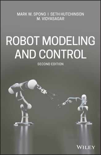
If a = (ax, ay, az) is a 3-vector, we define the skew symmetric matrix S(a) as
Example 4.1.
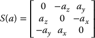
Denote by i, j, and k the three unit basis coordinate vectors,
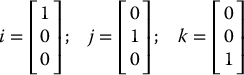
The skew-symmetric matrices S(i), S(j), and S(k) are given by
Skew-symmetric matrices possess several properties that will prove useful for subsequent derivations.1 Among these properties are Suppose now that a rotation matrix R is a function of the single variable θ. Hence, R = R(θ) ∈ SO(3) for every θ. Since R is orthogonal for all θ it follows that
Differentiating both sides of Equation (4.10) with respect to θ using the product rule gives
Let us define the matrix S as
Then the transpose of S is
Equation (4.11) says that
In other words, the matrix S defined by Equation (4.12) is skew-symmetric. Multiplying both sides of Equation (4.12) on the right by R and using the fact that RTR = I yields
Equation (4.15) is very important. It says that computing the derivative of the rotation matrix R is equivalent to a matrix multiplication by a skew-symmetric matrix S. The most commonly encountered situation is the case where R is a basic rotation matrix or a product of basic rotation matrices. Example 4.2. If Thus, we have shown that
Similar computations show that
Example 4.3. Let
4.2.1 Properties of Skew-Symmetric Matrices
![]()
![]() and scalars α and β.
and scalars α and β.![]() ,
,
![]()
![]()
![]()
![]()
![]()
![]() be an arbitrary vector. Then
be an arbitrary vector. Then

4.2.2 The Derivative of a Rotation Matrix
![]()
![]()
![]()

![]()
![]()
![]() , the basic rotation matrix given by Equation (2.7), then direct computation shows that
, the basic rotation matrix given by Equation (2.7), then direct computation shows that

![]()
![]()
![]() be a rotation about the axis defined by k = (k1, k2, k3) as in Equation (2.44). It is easy to show using Rodrigues’ formula that
be a rotation about the axis defined by k = (k1, k2, k3) as in Equation (2.44). It is easy to show using Rodrigues’ formula that
![]()
4.3 Angular Velocity: The General Case
We now consider the general case of angular velocity about an arbitrary, possibly moving, axis. Suppose that a rotation matrix R is time-varying, so that R = R(t) ∈ SO(3) for every ![]() . Assuming that R(t) is continuously differentiable as a function of t, an argument identical to the one in the previous section shows that the time derivative
. Assuming that R(t) is continuously differentiable as a function of t, an argument identical to the one in the previous section shows that the time derivative ![]() of R(t) can be written as
of R(t) can be written as
where the matrix S(ω(t)) is skew symmetric. The vector ω(t) is the angular velocity of the rotating frame with respect to the fixed frame at time t. To see that ω is the angular velocity vector, consider a point p rigidly attached to a moving frame. The coordinates of p relative to the fixed frame are given by ![]() . Differentiating this expression we obtain
. Differentiating this expression we obtain
which shows that ω is indeed the traditional angular velocity vector.
Equation (4.18) shows the relationship between angular velocity and the derivative of a rotation matrix. In particular, if the instantaneous orientation of a frame o1x1y1z1 with respect to a frame o0x0y0z0 is given by ![]() , then the angular velocity of frame o1x1y1z1 is directly related to the derivative of
, then the angular velocity of frame o1x1y1z1 is directly related to the derivative of ![]() by Equation (4.18). When there is a possibility of ambiguity, we will use the notation ωi, j to denote the angular velocity that corresponds to the derivative of the rotation matrix
by Equation (4.18). When there is a possibility of ambiguity, we will use the notation ωi, j to denote the angular velocity that corresponds to the derivative of the rotation matrix ![]() . Since ω is a free vector, we can express it with respect to any coordinate system of our choosing. As usual we use a superscript to denote the reference frame. For example, ω01, 2 would give the angular velocity that corresponds to the derivative of
. Since ω is a free vector, we can express it with respect to any coordinate system of our choosing. As usual we use a superscript to denote the reference frame. For example, ω01, 2 would give the angular velocity that corresponds to the derivative of ![]() , expressed in coordinates relative to frame o0x0y0z0. In cases where the angular velocities specify rotation relative to the base frame, we will often simplify the subscript, for example, using ω2 to represent the angular velocity that corresponds to the derivative of
, expressed in coordinates relative to frame o0x0y0z0. In cases where the angular velocities specify rotation relative to the base frame, we will often simplify the subscript, for example, using ω2 to represent the angular velocity that corresponds to the derivative of ![]() .
.
Example 4.4.
Suppose that ![]() . Then
. Then ![]() is computed using the chain rule as
is computed using the chain rule as
in which ![]() is the angular velocity. Note, i = (1, 0, 0).
is the angular velocity. Note, i = (1, 0, 0).
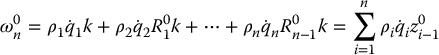
4.4 Addition of Angular Velocities
We are often interested in finding the resultant angular velocity due to the relative rotation of several coordinate frames. We now derive the expressions for the composition of angular velocities of two moving frames o1x1y1z1 and o2x2y2z2 relative to the fixed frame o0x0y0z0. For now, we assume that the three frames share a common origin. Let the relative orientations of the frames o1x1y1z1 and o2x2y2z2 be given by the rotation matrices ![]() and
and ![]() (both time-varying).
(both time-varying).
In the derivations that follow, we will use the notation ![]() to denote the angular velocity vector that corresponds to the time derivative of the rotation matrix Rij. Since we can express this vector relative to the coordinate frame of our choosing, we again use a superscript to define the reference frame. Thus,
to denote the angular velocity vector that corresponds to the time derivative of the rotation matrix Rij. Since we can express this vector relative to the coordinate frame of our choosing, we again use a superscript to define the reference frame. Thus, ![]() would denote the angular velocity vector corresponding to the derivative of Rij, expressed relative to frame k.
would denote the angular velocity vector corresponding to the derivative of Rij, expressed relative to frame k.
As in Chapter 2,
Taking derivatives of both sides of Equation (4.20) with respect to time yields
Using Equation (4.18), the term ![]() on the left-hand side of Equation (4.21) can be written
on the left-hand side of Equation (4.21) can be written
In this expression, ![]() denotes the total angular velocity experienced by frame o2x2y2z2. This angular velocity results from the combined rotations expressed by
denotes the total angular velocity experienced by frame o2x2y2z2. This angular velocity results from the combined rotations expressed by ![]() and
and ![]() .
.
The first term on the right-hand side of Equation (4.21) is simply
In this equation, ![]() denotes the angular velocity of frame o1x1y1z1 that results from the changing
denotes the angular velocity of frame o1x1y1z1 that results from the changing ![]() , and this angular velocity vector is expressed relative to the coordinate system o0x0y0z0.
, and this angular velocity vector is expressed relative to the coordinate system o0x0y0z0.
Let us examine the second term on the right-hand side of Equation (4.21). Using Equation (4.8) we have
In this equation, ![]() denotes the angular velocity of frame o2x2y2z2 that corresponds to the changing
denotes the angular velocity of frame o2x2y2z2 that corresponds to the changing ![]() , expressed relative to the coordinate system o1x1y1z1. Thus, the product
, expressed relative to the coordinate system o1x1y1z1. Thus, the product ![]() expresses this angular velocity relative to the coordinate system o0x0y0z0. In other words, R01ω11, 2 gives the coordinates of the free vector ω1, 2 with respect to frame 0.
expresses this angular velocity relative to the coordinate system o0x0y0z0. In other words, R01ω11, 2 gives the coordinates of the free vector ω1, 2 with respect to frame 0.
Now, combining the above expressions we have shown that
Since S(a) + S(b) = S(a + b), we see that
In other words, the angular velocities can be added once they are expressed relative to the same coordinate frame, in this case o0x0y0z0.
The above reasoning can be extended to any number of coordinate systems. In particular, suppose that we are given
Extending the above reasoning we obtain
in which
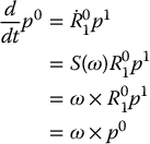
4.5 Linear Velocity of a Point Attached to a Moving Frame
We now consider the linear velocity of a point that is rigidly attached to a moving frame. Suppose the point p is rigidly attached to the frame o1x1y1z1, and that o1x1y1z1 is rotating relative to the frame o0x0y0z0. Then the coordinates of p with respect to the frame o0x0y0z0 are given by
The velocity ![]() is then given by the product rule for differentiation as
is then given by the product rule for differentiation as

which is the familiar expression for the velocity in terms of the vector cross product. Note that Equation (4.32) follows from the fact that p is rigidly attached to frame o1x1y1z1, and therefore its coordinates relative to frame o1x1y1z1 do not change, giving ![]() .
.
Now, suppose that the motion of the frame o1x1y1z1 relative to o0x0y0z0 is more general. Suppose that the homogeneous transformation relating the two frames is time-dependent, so that
For simplicity we omit the argument t and the subscripts and superscripts on ![]() and
and ![]() , and write
, and write
Differentiating the above expression using the product rule gives
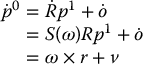
where ![]() is the vector from o1 to p expressed in the orientation of the frame o0x0y0z0, and v is the rate at which the origin o1 is moving.
is the vector from o1 to p expressed in the orientation of the frame o0x0y0z0, and v is the rate at which the origin o1 is moving.
If the point ![]() is moving relative to the frame o1x1y1z1, then we must add to the term v the term
is moving relative to the frame o1x1y1z1, then we must add to the term v the term ![]() , which is the rate of change of the coordinates
, which is the rate of change of the coordinates ![]() expressed in the frame o0x0y0z0.
expressed in the frame o0x0y0z0.
4.6 Derivation of the Jacobian
Consider an n-link manipulator with joint variables q1, …, qn . Let
denote the transformation from the end-effector frame to the base frame, where q = (q1, …, qn) is the vector of joint variables. As the robot moves about, both the joint variables qi and the end-effector position ![]() and orientation
and orientation ![]() will be functions of time. The objective of this section is to relate the linear and angular velocity of the end effector to the vector of joint velocities
will be functions of time. The objective of this section is to relate the linear and angular velocity of the end effector to the vector of joint velocities ![]() . Let
. Let
define the angular velocity vector ![]() of the end effector, and let
of the end effector, and let
denote the linear velocity of the end effector. We seek expressions of the form
where Jv and Jω are 3 × n matrices. We may write Equations (4.39) and (4.40) together as
in which ξ and J are given by
The vector ξ is sometimes called a body velocity. Note that this velocity vector is not the derivative of a position variable, since the angular velocity vector is not the derivative of any particular time-varying quantity. The matrix J is called the manipulator Jacobian or Jacobian for short. Note that J is a 6 × n matrix where n is the number of links. We next derive a simple expression for the Jacobian of any manipulator.
4.6.1 Angular Velocity
Recall from Equation (4.29) that angular velocities can be added as free vectors, provided that they are expressed relative to a common coordinate frame. Thus, we can determine the angular velocity of the end effector relative to the base by expressing the angular velocity contributed by each joint in the orientation of the base frame and then summing these.
If the ith joint is revolute, then the ith joint variable qi equals θi and the axis of rotation is zi − 1. Slightly abusing notation, let ![]() represent the angular velocity of link i that is imparted by the rotation of joint i, expressed relative to frame oi − 1xi − 1yi − 1zi − 1. This angular velocity is expressed in the frame i − 1 by
represent the angular velocity of link i that is imparted by the rotation of joint i, expressed relative to frame oi − 1xi − 1yi − 1zi − 1. This angular velocity is expressed in the frame i − 1 by
in which, as above, k is the unit coordinate vector (0, 0, 1).
If the ith joint is prismatic, then the motion of frame i relative to frame i − 1 is a translation and
Thus, if joint i is prismatic, the angular velocity of the end effector does not depend on qi, which now equals di.
Therefore, the overall angular velocity of the end effector, ![]() , in the base frame is determined by Equation (4.29) as
, in the base frame is determined by Equation (4.29) as
in which ρi is equal to 1 if joint i is revolute and 0 if joint i is prismatic, since
Of course, ![]() .
.
The lower half of the Jacobian Jω, in Equation (4.42) is thus given as
Note that, in this equation, we have omitted the superscripts for the unit vectors along the z-axes, since these are all referenced to the world frame. In the remainder of the chapter we will follow this convention when there is no ambiguity concerning the reference frame.
4.6.2 Linear Velocity
The linear velocity of the end effector is just ![]() . By the chain rule for differentiation
. By the chain rule for differentiation

Thus, we see that the ith column of Jv, which we denote as ![]() is given by
is given by

Furthermore, this expression is just the linear velocity of the end effector that would result if ![]() were equal to one and the other
were equal to one and the other ![]() were zero. In other words, the ith column of the Jacobian can be generated by holding all joints but the ith joint fixed and actuating the ith at unit velocity. This observation leads to a simple and intuitive derivation of the linear velocity Jacobian as we now show. We now consider the two cases of prismatic and revolute joints separately.
were zero. In other words, the ith column of the Jacobian can be generated by holding all joints but the ith joint fixed and actuating the ith at unit velocity. This observation leads to a simple and intuitive derivation of the linear velocity Jacobian as we now show. We now consider the two cases of prismatic and revolute joints separately.
Case 1: Prismatic Joints
Figure 4.1 illustrates the case when all joints are fixed except a single prismatic joint. Since joint i is prismatic, it imparts a pure translation to the end effector. The direction of translation is parallel to the axis zi − 1 and the magnitude of the translation is ![]() , where di is the DH joint variable. Thus, in the orientation of the base frame we have
, where di is the DH joint variable. Thus, in the orientation of the base frame we have

in which di is the joint variable for prismatic joint i. Thus, for the case of prismatic joints, after dropping the superscripts we have
Figure 4.1 Motion of the end effector due to prismatic joint i.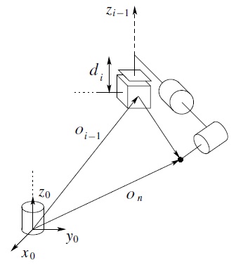
Case 2: Revolute Joints
Figure 4.2 illustrates the case when all joints are fixed except a single revolute joint. Since joint i is revolute, we have qi = θi. Referring to Figure 4.2 and assuming that all joints are fixed except joint i, we see that the linear velocity of the end effector is simply of the form ω × r, where
and
Figure 4.2 Motion of the end effector due to revolute joint i.
Thus, putting these together and expressing the coordinates relative to the base frame, for a revolute joint we obtain
in which we have omitted the zero superscripts following our convention.
4.6.5 Combining the Linear and Angular Velocity Jacobians
As we have seen in the preceding section, the upper half of the Jacobian Jv is given as
in which the ith column ![]() is
is
The lower half of the Jacobian is given as
in which the ith column ![]() is
is
The above formulas make the determination of the Jacobian of any manipulator simple since all of the quantities needed are available once the forward kinematics are worked out. Indeed, the only quantities needed to compute the Jacobian are the unit vectors zi and the coordinates of the origins o1, …, on. A moment’s reflection shows that the coordinates for zi with respect to the base frame are given by the first three elements in the third column of ![]() while oi is given by the first three elements of the fourth column of
while oi is given by the first three elements of the fourth column of ![]() . Thus, only the third and fourth columns of the
. Thus, only the third and fourth columns of the ![]() matrices are needed in order to evaluate the Jacobian according to the above formulas.
matrices are needed in order to evaluate the Jacobian according to the above formulas.
The above procedure works not only for computing the velocity of the end effector but also for computing the velocity of any point on the manipulator. This will be important in Chapter 6 when we will need to compute the velocity of the center of mass of the various links in order to derive the dynamic equations of motion.
Example 4.5. (Two-Link Planar Manipulator)
Consider the two-link planar manipulator of Example 3.3.1. Since both joints are revolute, the Jacobian matrix, which in this case is 6 × 2, is of the form
The various quantities above are easily seen to be
Performing the required calculations then yields

It is easy to see how the above Jacobian compares with Equation (1.1) derived in Chapter 1. The first two rows of Equation (4.62) are exactly the 2 × 2 Jacobian of Chapter 1 and give the linear velocity of the origin o2 relative to the base. The third row in Equation (4.62) is the linear velocity in the direction of z0, which is of course always zero in this case. The last three rows represent the angular velocity of the final frame, which is simply a rotation about the vertical axis at the rate ![]() .
.
Example 4.6. (Jacobian for an Arbitrary Point on a Link).
Consider the three-link planar manipulator of Figure 4.3. Suppose we wish to compute the linear velocity v and the angular velocity ω of the center of link 2 as shown.
In this case we have that
which is merely the usual Jacobian with oc in place of on. Note that the third column of the Jacobian is zero, since the velocity of the second link is unaffected by motion of the third link.2 Note that in this case the vector oc must be computed as it is not given directly by the T matrices (Problem 4–11).
Example 4.7. (Stanford Manipulator).
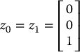
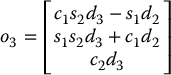
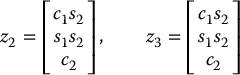
Consider the Stanford Manipulator of Example 3.3.5 with its associated Denavit–Hartenberg coordinate frames. Note that joint 3 is prismatic and that o3 = o4 = o5 as a consequence of the spherical wrist and the frame assignment. Denoting this common origin by o we see that the columns of the Jacobian have the form
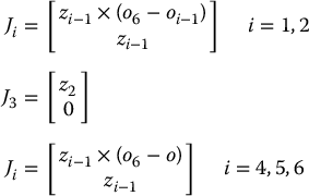
Now, using the A matrices given by Equations (3.18)–(3.20) and the T matrices formed as products of the A matrices, these quantities are easily computed as follows. First, oj is given by the first three entries of the last column of ![]() , with o0 = (0, 0, 0) = o1. The vector zj is given as
, with o0 = (0, 0, 0) = o1. The vector zj is given as ![]() where
where ![]() is the rotational part of
is the rotational part of ![]() . Thus, it is only necessary to compute the matrices
. Thus, it is only necessary to compute the matrices ![]() to calculate the Jacobian. Carrying out these calculations one obtains the following expressions for the Stanford Manipulator:
to calculate the Jacobian. Carrying out these calculations one obtains the following expressions for the Stanford Manipulator:

The various z-axes are given as

The Jacobian of the Stanford Manipulator is now given by combining these expressions according to the given formulas (Problem 4–17).
Example 4.8. (SCARA Manipulator)
We will now derive the Jacobian of the SCARA manipulator of Example 3.3.6. This Jacobian is a 6 × 4 matrix since the SCARA has only four degrees of freedom. As before we need only compute the matrices ![]() , where the A matrices are given by Equations (3.22) and (3.23).
, where the A matrices are given by Equations (3.22) and (3.23).
Since joints 1, 2, and 4 are revolute and joint 3 is prismatic, and since o4 − o3 is parallel to z3 (and thus, z3 × (o4 − o3) = 0), the Jacobian is of the form
The origins of the DH frames are given by

Similarly z0 = z1 = k, and z2 = z3 = −k. Therefore the Jacobian of the SCARA Manipulator is
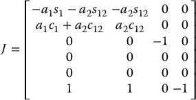
Figure 4.3 Finding the velocity of link 2 of a 3-link planar robot.
4.7 The Tool Velocity
Many tasks require that a tool be attached to the end effector. In such cases, it is necessary to relate the velocity of the tool frame to the velocity of the end-effector frame. Suppose that the tool is rigidly attached to the end effector, and the fixed spatial relationship between the end effector and the tool frame is given by the constant homogeneous transformation matrix
We will assume that the end effector velocity is given and expressed in coordinates relative to the end-effector frame, that is, we are given ξ66. In this section we will derive the velocity of the tool expressed in coordinates relative to the tool frame, that is, we will derive ξtooltool.
Since the two frames are rigidly attached, the angular velocity of the tool frame is the same as the angular velocity of the end-effector frame. To see this, simply compute the angular velocities of each frame by taking the derivatives of the appropriate rotation matrices. Since R is constant and R0tool = R06R, we have
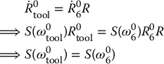
Thus, ωtool = ω6, and to obtain the tool angular velocity relative to the tool frame we apply a rotational transformation
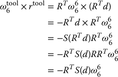
If the end-effector frame is moving with body velocity ξ = (v6, ω6), then the linear velocity of the origin of the tool frame, which is rigidly attached to the end-effector frame, is given by
where r is the vector from the origin of the end-effector frame to the origin of the tool frame. From Equation (4.74), we see that d gives the coordinates of the origin of the tool frame with respect to the end-effector frame, and therefore we can express r in coordinates relative to the tool frame as rtool = RTd. Thus, we write ω6 × r in coordinates with respect to the tool frame as
To express the free vector v66 in coordinates relative to the tool frame, we apply the rotational transformation
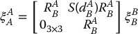
Combining Equations (4.76), (4.77), and (4.78) to obtain the linear velocity of the tool frame and using Equation (4.75) for the angular velocity of the tool frame, we have

which can be written as the matrix equation
In many cases, it is useful to solve the inverse problem: compute the required end effector-velocity to produce a desired tool velocity. Since
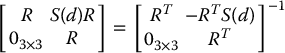
(Problem 4–18) we can solve Equation (4.79) for ξ66, obtaining
This gives the general expression for transforming velocities between two rigidly attached moving frames
4.8 The Analytical Jacobian
The Jacobian matrix derived above is sometimes called the geometric Jacobian to distinguish it from the analytical Jacobian, denoted Ja(q), which is based on a minimal representation for the orientation of the end-effector frame. Let
denote the end-effector pose, where d(q) is the usual vector from the origin of the base frame to the origin of the end-effector frame and α denotes a minimal representation for the orientation of the end-effector frame relative to the base frame. For example, let α = (ϕ, θ, ψ) be a vector of Euler angles as defined in Chapter 2. Then we seek an expression of the form
to define the analytical Jacobian.
It can be shown (Problem 4–7) that, if R = Rz, ϕRy, θRz, ψ is the Euler angle transformation, then
in which ω defining the angular velocity is given by


The components of ω are called nutation,spin, and precession, respectively. Combining the above relationship with the previous definition of the Jacobian
yields
Thus, the analytical Jacobian, Ja(q), may be computed from the geometric Jacobian as
provided ![]() .
.
In the next section we discuss the notion of Jacobian singularities, which are configurations where the Jacobian loses rank. Singularities of the matrix B(α) are called representational singularities. It can easily be shown (Problem 4–19) that B(α) is invertible provided sθ ≠ 0. This means that the singularities of the analytical Jacobian include the singularities of the geometric Jacobian, J, as defined in the next section, together with the representational singularities.
4.9 Singularities
The 6 × n Jacobian J(q) defines a mapping
between the vector ![]() of joint velocities and the vector ξ = (v, ω) of end-effector velocities. This implies that all possible end-effector velocities are linear combinations of the columns of the Jacobian matrix,
of joint velocities and the vector ξ = (v, ω) of end-effector velocities. This implies that all possible end-effector velocities are linear combinations of the columns of the Jacobian matrix,
For example, for the two-link planar arm, the Jacobian matrix given in Equation (4.62) has two columns. It is easy to see that the linear velocity of the end effector must lie in the xy-plane, since neither column has a nonzero entry for the third row. Since ![]() , it is necessary that J have six linearly independent columns for the end effector to be able to achieve any arbitrary velocity (see Appendix B).
, it is necessary that J have six linearly independent columns for the end effector to be able to achieve any arbitrary velocity (see Appendix B).
The rank of a matrix is the number of linearly independent columns (or rows) in the matrix. Thus, when rank J = 6, the end effector can execute any arbitrary velocity. For a matrix ![]() , it is always the case that rank J ⩽ min (6, n). For example, for the two-link planar arm, we always have rank J ⩽ 2, while for an anthropomorphic arm with spherical wrist we always have rank J ⩽ 6.
, it is always the case that rank J ⩽ min (6, n). For example, for the two-link planar arm, we always have rank J ⩽ 2, while for an anthropomorphic arm with spherical wrist we always have rank J ⩽ 6.
The rank of a matrix is not necessarily constant. Indeed, the rank of the manipulator Jacobian matrix will depend on the configuration q. Configurations for which rank J(q) is less than its maximum value are called singularities or singular configurations.
Identifying manipulator singularities is important for several reasons.
- Singularities represent configurations from which certain directions of motion may be unattainable.
- At singularities, bounded end-effector velocities may correspond to unbounded joint velocities.
- At singularities, bounded joint torques may correspond to unbounded end-effector forces and torques. (We will see this in Chapter 10.)
- Singularities often correspond to points on the boundary of the manipulator workspace, that is, to points of maximum reach of the manipulator.
- Singularities correspond to points in the manipulator workspace that may be unreachable under small perturbations of the link parameters, such as length, offset, etc.
There are a number of methods that can be used to determine the singularities of the Jacobian. In this chapter, we will exploit the fact that a square matrix is singular when its determinant is equal to zero. In general, it is difficult to solve the nonlinear equation ![]() . Therefore, we now introduce the method of decoupling singularities, which is applicable whenever, for example, the manipulator is equipped with a spherical wrist.
. Therefore, we now introduce the method of decoupling singularities, which is applicable whenever, for example, the manipulator is equipped with a spherical wrist.
4.9.1 Decoupling of Singularities
We saw in Chapter 3 that a set of forward kinematic equations can be derived for any manipulator by attaching a coordinate frame rigidly to each link in any manner that we choose, computing a set of homogeneous transformations relating the coordinate frames, and multiplying them together as needed. The DH convention is merely a systematic way to do this. Although the resulting equations are dependent on the coordinate frames chosen, the manipulator configurations themselves are geometric quantities, independent of the frames used to describe them. Recognizing this fact allows us to decouple the determination of singular configurations, for those manipulators with spherical wrists, into two simpler problems. The first is to determine so-called arm singularities, that is, singularities resulting from motion of the arm, which consists of the first three or more links, while the second is to determine the wrist singularities resulting from motion of the spherical wrist.
Consider the case that n = 6, that is, the manipulator consists of a 3-DOF arm with a 3-DOF spherical wrist. In this case the Jacobian is a 6 × 6 matrix and a configuration q is singular if and only if
If we now partition the Jacobian J into 3 × 3 blocks as
then, since the final three joints are always revolute
Since the wrist axes intersect at a common point o, if we choose the coordinate frames so that o3 = o4 = o5 = o6 = o, then JO becomes
In this case the Jacobian matrix has the block triangular form
with determinant
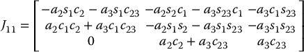
where J11 and J22 are each 3 × 3 matrices. J11 has ith column zi − 1 × (o − oi − 1) if joint i is revolute, and zi − 1 if joint i is prismatic, while
Therefore the set of singular configurations of the manipulator is the union of the set of arm configurations satisfying ![]() and the set of wrist configurations satisfying
and the set of wrist configurations satisfying ![]() . Note that this form of the Jacobian does not necessarily give the correct relation between the velocity of the end effector and the joint velocities. It is intended only to simplify the determination of singularities.
. Note that this form of the Jacobian does not necessarily give the correct relation between the velocity of the end effector and the joint velocities. It is intended only to simplify the determination of singularities.
4.9.2 Wrist Singularities
We can now see from Equation (4.96) that a spherical wrist is in a singular configuration whenever the vectors z3, z4, and z5 are linearly dependent. Referring to Figure 4.4 we see that this happens when the joint axes z3 and z5 are collinear, that is, when θ5 = 0 or π. These are the only singularities of the spherical wrist, and they are unavoidable without imposing mechanical limits on the wrist design to restrict its motion in such a way that z3 and z5 are prevented from lining up. In fact, when any two revolute-joint axes are collinear a singularity results, since an equal and opposite rotation about the axes results in no net motion of the end effector.
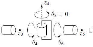
Figure 4.4 Spherical wrist singularity.
4.9.3 Arm Singularities
To investigate arm singularities we need only to compute ![]() , which is done using Equation (4.56) but with the wrist center o in place of on. In the remainder of this section, we will determine the singularities for three common arms, the elbow manipulator, the spherical manipulator and the SCARA manipulator.
, which is done using Equation (4.56) but with the wrist center o in place of on. In the remainder of this section, we will determine the singularities for three common arms, the elbow manipulator, the spherical manipulator and the SCARA manipulator.
Example 4.9. (Elbow Manipulator Singularities).
Consider the three-link articulated manipulator with coordinate frames attached as shown in Figure 4.5. It is left as an exercise (Problem 4–12) to show that
and that the determinant of J11 is
We see from Equation (4.98) that the elbow manipulator is in a singular configuration when
and whenever
The situation of Equation (4.99) is shown in Figure 4.6 and arises when the elbow is fully extended or fully retracted as shown. The second situation of Equation (4.100) is shown in Figure 4.7. This configuration occurs when the wrist center intersects the axis of the base rotation, z0. As we saw in Chapter 5, there are infinitely many singular configurations and infinitely many solutions to the inverse position kinematics when the wrist center is along this axis.
For an elbow manipulator with an offset, as shown in Figure 4.8, the wrist center cannot intersect z0, which corroborates our earlier statement that points reachable at singular configurations may not be reachable under arbitrarily small perturbations of the manipulator parameters, in this case an offset in either the elbow or the shoulder.
Example 4.10. (Spherical Manipulator).
Consider the spherical arm of Figure 4.9. This manipulator is in a singular configuration when the wrist center intersects z0 as shown since, as before, any rotation about the base leaves this point fixed.
Example 4.11. (SCARA Manipulator).
We have already derived the complete Jacobian for the SCARA manipulator. This Jacobian is simple enough to be used directly rather than deriving the modified Jacobian as we have done above. Referring to Figure 4.10 we can see geometrically that the only singularity of the SCARA arm is when the elbow is fully extended or fully retracted. Indeed, since the portion of the Jacobian of the SCARA governing arm singularities is given as
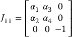
where
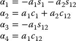
we see that the rank of J11 will be less than three when α1α4 − α2α3 = 0. It is easy to compute this quantity and show that it is equivalent to (Problem 4–14)
Note the similarities between this case and the singularities for the elbow manipulator shown in Figure 4.6. In each case, the relevant portion of the arm is merely a two-link planar manipulator. As can be seen from Equation (4.62), the Jacobian for the two-link planar manipulator loses rank when θ2 = 0 or π.

Figure 4.5 Elbow manipulator.
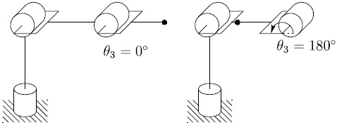
Figure 4.6 Elbow singularities of the elbow manipulator.
Figure 4.7 Singularity of the elbow manipulator with no offsets.

Figure 4.8 Elbow manipulator with an offset at the elbow.
Figure 4.9 Singularity of spherical manipulator with no offsets.

Figure 4.10 SCARA manipulator singularity.
4.10 Static Force/Torque Relationships
Interaction of the manipulator with the environment produces forces and moments at the end effector or tool. These, in turn, produce torques at the joints of the robot.3 In this section we discuss the role of the manipulator Jacobian in the quantitative relationship between the end-effector forces and joint torques. This relationship is important for the development of path planning methods in Chapter 7, the derivation of the dynamic equations in Chapter 6 and in the design of force control algorithms in Chapter 10. We can state the main result concisely as follows.
Let F = (Fx, Fy, Fz, nx, ny, nz) represent the vector of forces and moments at the end effector. Let τ denote the corresponding vector of joint torques. Then F and τ are related by
where JT(q) is the transpose of the manipulator Jacobian.
An easy way to derive this relationship is through the so-called principle of virtual work. We will defer a detailed discussion of the principle of virtual work until Chapter 6, where we will introduce the notions of generalized coordinates, holonomic constraints, and virtual constraints in more detail. However, we can give a somewhat informal justification in this section as follows. Let δX and δq represent infinitesimal displacements in the task space and joint space, respectively. These displacements are called virtual displacements if they are consistent with any constraints imposed on the system. For example, if the end effector is in contact with a rigid wall, then the virtual displacements in position are tangent to the wall. These virtual displacements are related through the manipulator JacobianJ(q) according to
The virtual work δw of the system is
Substituting Equation (4.105) into Equation (4.106) yields
The principle of virtual work says, in effect, that the quantity given by Equation (4.107) is equal to zero if the manipulator is in equilibrium. This leads to the relationship given by Equation (4.104). In other words, the end-effector forces are related to the joint torques by the transpose of the manipulator Jacobian.
Example 4.12.
Consider the two-link planar manipulator of Figure 4.11, with a force F applied at the end of link two as shown. The Jacobian of this manipulator is given by Equation (4.62). The resulting joint torques τ = (τ1, τ2) are then given as
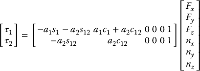
Figure 4.11 Two-link planar robot.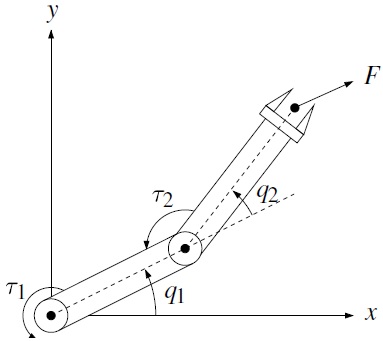
4.11 Inverse Velocity and Acceleration
The Jacobian relationship
specifies the end-effector velocity that will result when the joints move with velocity ![]() . The inverse velocity problem is the problem of finding the joint velocities
. The inverse velocity problem is the problem of finding the joint velocities ![]() that produce the desired end-effector velocity. It is perhaps a bit surprising that the inverse velocity relationship is conceptually simpler than the inverse position relationship. When the Jacobian is square and nonsingular, this problem can be solved by simply inverting the Jacobian matrix to give
that produce the desired end-effector velocity. It is perhaps a bit surprising that the inverse velocity relationship is conceptually simpler than the inverse position relationship. When the Jacobian is square and nonsingular, this problem can be solved by simply inverting the Jacobian matrix to give
For manipulators that do not have exactly six joints, the Jacobian cannot be inverted. In this case there will be a solution to Equation (4.109) if and only if ξ lies in the range space of the Jacobian. This can be determined by the following simple rank test. A vector ξ belongs to the range of J if and only if
In other words, Equation (4.109) may be solved for ![]() provided that the rank of the augmented matrix[J(q)∣ξ] is the same as the rank of the Jacobian J(q). This is a standard result from linear algebra, and several algorithms exist, such as Gaussian elimination, for solving such systems of linear equations.
provided that the rank of the augmented matrix[J(q)∣ξ] is the same as the rank of the Jacobian J(q). This is a standard result from linear algebra, and several algorithms exist, such as Gaussian elimination, for solving such systems of linear equations.
For the case when n > 6 we can solve for ![]() using the right pseudoinverse of J. We leave it as an exercise to show (Problem 4–20) that a solution to Equation (4.109) is given by
using the right pseudoinverse of J. We leave it as an exercise to show (Problem 4–20) that a solution to Equation (4.109) is given by
in which ![]() is an arbitrary vector.
is an arbitrary vector.
In general, for m < n, (I − J+J) ≠ 0, and all vectors of the form (I − J+J)b lie in the null space of J. This means that, if ![]() is a joint velocity vector such that
is a joint velocity vector such that ![]() , then when the joints move with velocity
, then when the joints move with velocity ![]() , the end effector will remain fixed since
, the end effector will remain fixed since ![]() . Thus, if
. Thus, if ![]() is a solution to Equation (4.109), then so is
is a solution to Equation (4.109), then so is ![]() with
with ![]() , for any value of b. If the goal is to minimize the resulting joint velocities, we choose b = 0 (Problem 4–20).
, for any value of b. If the goal is to minimize the resulting joint velocities, we choose b = 0 (Problem 4–20).
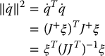
We can construct the right pseudoinverse of J using its singular value decomposition (see Appendix B).
We can apply a similar approach when the analytical Jacobian is used in place of the manipulator Jacobian. Recall from Equation (4.83) that the joint velocities and the end-effector velocities are related by the analytical Jacobian as
Thus, the inverse velocity problem becomes one of solving the linear system given by Equation (4.113), which can be accomplished as above for the manipulator Jacobian.
Differentiating Equation (4.113) yields an expression for the acceleration
Thus, given a vector ![]() of end-effector accelerations, the instantaneous joint acceleration vector
of end-effector accelerations, the instantaneous joint acceleration vector ![]() is given as a solution of
is given as a solution of
For 6-DOF manipulators the inverse velocity and acceleration equations can therefore be written as
and
provided ![]() .
.
4.12 Manipulability
For a specific value of q, the Jacobian relationship defines the linear system given by ![]() . We can think of J as scaling the input
. We can think of J as scaling the input ![]() to produce the output ξ. It is often useful to characterize quantitatively the effects of this scaling. Often, in systems with a single input and a single output, this kind of characterization is given in terms of the so-called impulse response of a system, which essentially characterizes how the system responds to a unit input. In this multidimensional case, the analogous concept is to characterize the output in terms of an input that has unit norm. Consider the set of all robot joint velocities
to produce the output ξ. It is often useful to characterize quantitatively the effects of this scaling. Often, in systems with a single input and a single output, this kind of characterization is given in terms of the so-called impulse response of a system, which essentially characterizes how the system responds to a unit input. In this multidimensional case, the analogous concept is to characterize the output in terms of an input that has unit norm. Consider the set of all robot joint velocities ![]() such that
such that
If we use the minimum norm solution ![]() , we obtain
, we obtain
The derivation of this is left as an exercise (Problem 4–21). Equation (4.118) gives us a quantitative characterization of the scaling effected by the Jacobian. In particular, if the manipulator Jacobian is full rank, that is, if rank J = m, then Equation (4.118) defines an m-dimensional ellipsoid that is known as the manipulability ellipsoid.If the input (joint velocity) vector has unit norm, then the output (end-effector velocity) will lie within the ellipsoid given by Equation (4.118). We can more easily see that Equation (4.118) defines an ellipsoid by replacing the Jacobian by its SVD J = UΣVT (see Appendix B) to obtain
in which

and σ1 ⩾ σ2… ⩾ σm ⩾ 0. The derivation of Equation (4.119) is left as an exercise (Problem 4–22). If we make the substitution w = UTξ, then Equation (4.119) can be written as

and it is clear that this is the equation for an axis-aligned ellipse in a new coordinate system that is obtained by rotation according to the orthogonal matrix UT. In the original coordinate system, the axes of the ellipsoid are given by the vectors σiui. The volume of the ellipsoid is given by
in which K is a constant that depends only on the dimension m of the ellipsoid. The manipulability measure is given by
Note that the constant K is not included in the definition of manipulability, since it is fixed once the task has been defined, that is, once the dimension of the task space has been fixed.
Now, consider the special case when the robot is not redundant, that is, ![]() . Recall that the determinant of a product is equal to the product of the determinants, and that a matrix and its transpose have the same determinant. Thus, we have
. Recall that the determinant of a product is equal to the product of the determinants, and that a matrix and its transpose have the same determinant. Thus, we have
in which λ1 ⩾ λ2 ⩾ ⋅⋅⋅ ⩾ λm are the eigenvalues of J. This leads to
The manipulability μ has the following properties.
- In general, μ = 0 holds if and only if rank(J) < m, that is, when J is not full rank.
- Suppose that there is some error in the measured velocity Δξ. We can bound the corresponding error in the computed joint velocity
 by
(4.124)
by
(4.124)
Example 4.13. (Two-link Planar Arm).
Consider the two-link planar arm and the task of positioning in the plane. The Jacobian is given by
and the manipulability is given by
Manipulability ellipsoids for several configurations of the two-link arm are shown in Figure 4.12.
We can use manipulability to determine the optimal configurations in which to perform certain tasks. In some cases it is desirable to perform a task in the configuration for which the end effector has the maximum manipulability. For the two-link arm the maximum manipulability is obtained for θ2 = ±π/2.
Manipulability can also be used to aid in the design of manipulators. For example, suppose that we wish to design a two-link planar arm whose total link length a1 + a2 is fixed. What values should be chosen for a1 and a2? If we design the robot to maximize the maximum manipulability, then we need to maximize μ = a1a2|s2|. We have already seen that the maximum is obtained when θ2 = ±π/2, so we need only find a1 and a2 to maximize the product a1a2. This is achieved when a1 = a2. Thus, to maximize manipulability, the link lengths should be chosen to be equal.

Figure 4.12 Manipulability ellipsoids are shown for several configurations of the two-link arm.
4.13 Chapter Summary
A moving coordinate frame has both a linear and an angular velocity. Linear velocity is associated to a moving point, while angular velocity is associated to a rotating frame. Thus, the linear velocity of a moving frame is merely the velocity of its origin. The angular velocity for a moving frame is related to the time derivative of the rotation matrix that describes the instantaneous orientation of the frame. In particular, if R(t) ∈ SO(3), then
and the vector ω(t) is the instantaneous angular velocity of the frame. The operator S gives a skew-symmetric matrix

The manipulator Jacobian relates the vector of joint velocities to the body velocity ξ = (vT, ω) of the end effector
This relationship can be written as two equations, one for linear velocity and one for angular velocity,
The ith column of the Jacobian matrix corresponds to the ith joint of the robot manipulator, and takes one of two forms depending on whether the ith joint is prismatic or revolute
It is often the case that a tool is attached to the end effector. When two frames are rigidly attached, their velocities are related by

and this relationship allows us to compute the required end effector velocity to achieve a desired tool velocity.
For a given parameterization of orientation, for example, Euler angles, the analytical Jacobian relates joint velocities to the time derivative of the pose parameters
in which d(q) is the usual vector from the origin of the base frame to the origin of the end-effector frame and α denotes a parameterization of the rotation matrix that specifies the orientation of the end-effector frame relative to the base frame. For the Euler angle parameterization, the analytical Jacobian is given by
in which

A configuration at which the Jacobian loses rank, that is, a configuration q such that rank J ⩽ max q rank J(q), is called a singularity. For a manipulator with a spherical wrist, the set of singular configurations includes singularities of the wrist (which are merely the singularities in the Euler angle parameterization) and singularities in the arm. The latter can be found by solving
with J11 the upper left 3 × 3 block of the manipulator Jacobian.
The Jacobian matrix can also be used to relate forces F applied at the end-effector frame to the induced joint torques τ
For nonsingular configurations, the Jacobian relationship can be used to find the joint velocities ![]() necessary to achieve a desired end-effector velocity ξ. The minimum norm solution is given by
necessary to achieve a desired end-effector velocity ξ. The minimum norm solution is given by
in which J+ = JT(JJT)− 1 is the right pseudoinverse of J.
Manipulability is defined by μ = σ1σ2⋅⋅⋅σm in which σi are the singular values for the manipulator Jacobian. The manipulability can be used to characterize the range of possible end-effector velocities for a given configuration q.
Problems
- Verify Equation (4.6) by direct calculation.
- Verify Equation (4.7) by direct calculation.
- Prove the assertion given in Equation (4.9) that R(a × b) = Ra × Rb, for R ∈ S0(3).
- Verify Equation (4.16) by direct calculation.
- Suppose that a = (1, −1, 2) and that R = Rx, 90. Show by direct calculation that RS(a)RT = S(Ra).
- Given R = Rx, θRy, ϕ, compute
 . Evaluate
  at
at  ,
,  .
. - Given the Euler angle transformation
show that
 where
The components of i, j, k, respectively, are called the nutation, spin, and precession.
where
The components of i, j, k, respectively, are called the nutation, spin, and precession.
- Repeat Problem 1–7 for the Roll-Pitch-Yaw transformation. In other words, find an explicit expression for ω such that
 , where R is given by Equation (2.39).
 - Section 2.5.1 described only the Z-Y-Z Euler angles. List all possible sets of Euler angles. Is it possible to have Z-Z-Y Euler angles? Why or why not?
- Two frames o0x0y0z0 and o1x1y1z1 are related by the homogeneous transformation
A particle has velocity v1(t) = (3, 1, 0) relative to frame o1x1y1z1. What is the velocity of the particle in frame o0x0y0z0?
- For the three-link planar manipulator of Example 4.6, compute the vector oc and derive the manipulator Jacobian matrix.
- Compute the Jacobian J11 for the 3-link elbow manipulator of Example 4.9 and show that it agrees with Equation (4.97). Show that the determinant of this matrix agrees with Equation (4.98).
- Compute the Jacobian J11 for the three-link spherical manipulator of Example 4.10.
- Use Equation (4.101) to show that the singularities of the SCARA manipulator are given by Equation (4.103).
- Find the 6 × 3 Jacobian for the three links of the cylindrical manipulator of Figure 3.7. Find the singular configurations for this arm.
- Repeat Problem 4–15 for the Cartesian manipulator of Figure 3.17.
- Complete the derivation of the Jacobian for the Stanford Manipulator from Example 4.7.
- Verify Equation (4.80) by direct computation.
- Show that B(α) given by Equation (4.86) is invertible provided sθ ≠ 0.
- Suppose that
 is a solution to Equation (4.109) for m < n.
- Show that
 is also a solution to Equation (4.109) for any
  .
. - Show that b = 0 gives the solution that minimizes the resulting joint velocities.
- Show that
- Verify Equation (4.118).
- Verify Equation (4.119).
Notes and References
Angular velocity is fundamentally related to the derivative of a rotation matrix, and therefore to the Lie algebra so(3). This relationship, and more generally the geometry of so(n), is explored in differential geometry texts, as well as in more advanced robotics texts such as [118].
The concept of a Jacobian matrix as a linear mapping from the tangent space of one manifold to the tangent space of a second manifold is also dealt with in differential geometry texts, and even in advanced calculus texts when one or both of the manifolds is a Euclidean space. The use of the geometric Jacobian matrix of Equation (4.41) to map joint velocities (which lie in the tangent space to the configuration space) to a velocity ξ = (v, ω) is not commonly found in mathematics texts (note that ξ is not itself the derivative of any quantity). However, most robotics texts include some description of the geometric Jacobian, including [134], [145], and [118].
Since the relationship between the end-effector velocity and the joint velocities is defined by a linear map, the inverse velocity problem is a special case of the more general problem of solving linear systems, a problem that is the subject of linear algebra. Algorithms for solving this problem can be found in a variety of texts, including [138] and [56].
The manipulability measure discussed in Section 4.12 is due to Yoshikawa [187].
Notes
- 1 These properties are consequences of the fact that so(3) is a Lie algebra, a vector space with a suitably defined product operation [15].
- 2 Note that we are treating only kinematic effects here. Reaction forces on link 2 due to the motion of link 3 will influence the motion of link 2. These dynamic effects are treated by the methods of Chapter 6.
- 3 Here, we consider the case of revolute joints. If the joints are prismatic, forces and moments at the end effector produce forces at the joints.