CHAPTER 1
INTRODUCTION
Robotics is a relatively young field of modern technology that crosses traditional engineering boundaries. Understanding the complexity of robots and their application requires knowledge of electrical engineering, mechanical engineering, systems and industrial engineering, computer science, economics, and mathematics. New disciplines of engineering, such as manufacturing engineering, applications engineering, and knowledge engineering have emerged to deal with the complexity of the field of robotics and factory automation. More recently, mobile robots are increasingly important for applications like autonomous vehicles and planetary exploration.
This book is concerned with fundamentals of robotics, including kinematics, dynamics, motion planning, computer vision, and control. Our goal is to provide an introduction to the most important concepts in these subjects as applied to industrial robot manipulators, mobile robots and other mechanical systems.
The term robot was first introduced by the Czech playwright Karel Čapek in his 1920 play Rossum’s Universal Robots, the word robota being the Czech word for worker. Since then the term has been applied to a great variety of mechanical devices, such as teleoperators, underwater vehicles, autonomous cars, drones, etc. Virtually anything that operates with some degree of autonomy under computer control has at some point been called a robot. In this text we will focus on two types of robots, namely industrial manipulators and mobile robots.
Industrial Manipulators
An industrial manipulator of the type shown in Figure 1.1 is essentially a mechanical arm operating under computer control. Such devices, though far from the robots of science fiction, are nevertheless extremely complex electromechanical systems whose analytical description requires advanced methods, presenting many challenging and interesting research problems.
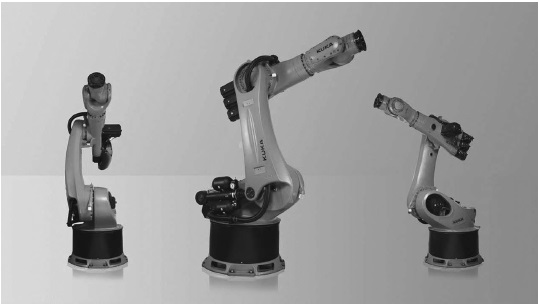
Figure 1.1 A six-axis industrial manipulator, the KUKA 500 FORTEC robot. (Photo courtesy of KUKA Robotics.)
An official definition of such a robot comes from the Robot Institute of America (RIA):
A robot is a reprogrammable, multifunctional manipulator designed to move material, parts, tools, or specialized devices through variable programmed motions for the performance of a variety of tasks.
The key element in the above definition is the reprogrammability, which gives a robot its utility and adaptability. The so-called robotics revolution is, in fact, part of the larger computer revolution.
Even this restricted definition of a robot has several features that make it attractive in an industrial environment. Among the advantages often cited in favor of the introduction of robots are decreased labor costs, increased precision and productivity, increased flexibility compared with specialized machines, and more humane working conditions as dull, repetitive, or hazardous jobs are performed by robots.
The industrial manipulator was born out of the marriage of two earlier technologies: teleoperators and numerically controlled milling machines. Teleoperators, or master-slave devices, were developed during the second world war to handle radioactive materials. Computer numerical control (CNC) was developed because of the high precision required in the machining of certain items, such as components of high performance aircraft. The first industrial robots essentially combined the mechanical linkages of the teleoperator with the autonomy and programmability of CNC machines.
The first successful applications of robot manipulators generally involved some sort of material transfer, such as injection molding or stamping, in which the robot merely attended a press to unload and either transfer or stack the finished parts. These first robots could be programmed to execute a sequence of movements, such as moving to a location A, closing a gripper, moving to a location B, etc., but had no external sensor capability. More complex applications, such as welding, grinding, deburring, and assembly, require not only more complex motion but also some form of external sensing such as vision, tactile, or force sensing, due to the increased interaction of the robot with its environment.
Figure 1.2 shows the estimated number of industrial robots worldwide between 2014 and 2020. In the future the market for service and medical robots will likely be even greater than the market for industrial robots. Service robots are defined as robots outside the manufacturing sector, such as robot vacuum cleaners, lawn mowers, window cleaners, delivery robots, etc. In 2018 alone, more than 30 million service robots were sold worldwide. The future market for robot assistants for elderly care and other medical robots will also be strong as populations continue to age.
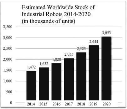
Figure 1.2 Estimated number of industrial robots worldwide 2014–2020. The industrial robot market has been growing around 14% per year. (Source: International Federation of Robotics 2018.)
Mobile Robots
Mobile robots encompass wheel and track driven robots, walking robots, climbing, swimming, crawling and flying robots. A typical wheeled mobile robot is shown in Figure 1.3. Mobile robots are used as household robots for vacuum cleaning and lawn mowing robots, as field robots for surveillance, search and rescue, environmental monitoring, forestry and agriculture, and other applications. Autonomous vehicles, for example self-driving cars and trucks, is an emerging area of robotics with great interest and promise.

Figure 1.3 Example of a typical mobile robot, the Fetch series. The figure on the right shows the mobile robot base with an attached manipulator arm. (Photo courtesy of Fetch Robotics.)
There are many other applications of robotics in areas where the use of humans is impractical or undesirable. Among these are undersea and planetary exploration, satellite retrieval and repair, the defusing of explosive devices, and work in radioactive environments. Finally, prostheses, such as artificial limbs, are themselves robotic devices requiring methods of analysis and design similar to those of industrial manipulators.
The science of robotics has grown tremendously over the past twenty years, fueled by rapid advances in computer and sensor technology as well as theoretical advances in control and computer vision. In addition to the topics listed above, robotics encompasses several areas not covered in this text such as legged robots, flying and swimming robots, grasping, artificial intelligence, computer architectures, programming languages, and computer-aided design. In fact, the new subject of mechatronics has emerged over the past four decades and, in a sense, includes robotics as a subdiscipline. Mechatronics has been defined as the synergistic integration of mechanics, electronics, computer science, and control, and includes not only robotics, but many other areas such as automotive control systems.
1.1 Mathematical Modeling of Robots
In this text we will be primarily concerned with developing and analyzing mathematical models for robots. In particular, we will develop methods to represent basic geometric aspects of robotic manipulation and locomotion. Equipped with these mathematical models, we will develop methods for planning and controlling robot motions to perform specified tasks. We begin here by describing some of the basic notation and terminology that we will use in later chapters to develop mathematical models for robot manipulators and mobile robots.
1.1.1 Symbolic Representation of Robot Manipulators
Robot manipulators are composed of links connected by joints to form a kinematic chain. Joints are typically rotary (revolute) or linear (prismatic). A revolute joint is like a hinge and allows relative rotation between two links. A prismatic joint allows a linear relative motion between two links. We denote revolute joints by R and prismatic joints by P, and draw them as shown in Figure 1.4. For example, a three-link arm with three revolute joints will be referred to as an RRR arm.
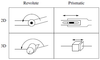
Figure 1.4 Symbolic representation of robot joints. Each joint allows a single degree of freedom of motion between adjacent links of the manipulator. The revolute joint (shown in 2D and 3D on the left) produces a relative rotation between adjacent links. The prismatic joint (shown in 2D and 3D on the right) produces a linear or telescoping motion between adjacent links.
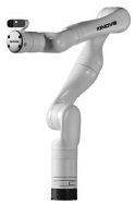
Figure 1.5 The Kinova® Gen3 Ultra lightweight arm, a 7-degree-of-freedom redundant manipulator. (Photo courtesy of Kinova, Inc.)
Each joint represents the interconnection between two links. We denote the axis of rotation of a revolute joint, or the axis along which a prismatic joint translates by zi if the joint is the interconnection of links i and i + 1. The joint variables, denoted by θ for a revolute joint and d for the prismatic joint, represent the relative displacement between adjacent links. We will make this precise in Chapter 3.
1.1.2 The Configuration Space
A configuration of a manipulator is a complete specification of the location of every point on the manipulator. The set of all configurations is called the configuration space. In the case of a manipulator arm, if we know the values for the joint variables (i.e., the joint angle for revolute joints, or the joint offset for prismatic joints), then it is straightforward to infer the position of any point on the manipulator, since the individual links of the manipulator are assumed to be rigid and the base of the manipulator is assumed to be fixed. Therefore, we will represent a configuration by a set of values for the joint variables. We will denote this vector of values by q, and say that the robot is in configuration q when the joint variables take on the values q1, …, qn, with qi = θi for a revolute joint and qi = di for a prismatic joint.
An object is said to have n degrees of freedom (DOF) if its configuration can be minimally specified by n parameters. Thus, the number of DOF is equal to the dimension of the configuration space. For a robot manipulator, the number of joints determines the number of DOF. A rigid object in three-dimensional space has six DOF: three for positioning and three for orientation. Therefore, a manipulator should typically possess at least six independent DOF. With fewer than six DOF the arm cannot reach every point in its work space with arbitrary orientation. Certain applications such as reaching around or behind obstacles may require more than six DOF. A manipulator having more than six DOF is referred to as a kinematically redundant manipulator.
1.1.3 The State Space
A configuration provides an instantaneous description of the geometry of a manipulator, but says nothing about its dynamic response. In contrast, the state of the manipulator is a set of variables that, together with a description of the manipulator’s dynamics and future inputs, is sufficient to determine the future time response of the manipulator. The state space is the set of all possible states. In the case of a manipulator arm, the dynamics are Newtonian, and can be specified by generalizing the familiar equation F = ma. Thus, a state of the manipulator can be specified by giving the values for the joint variables q and for the joint velocities ![]() (acceleration is related to the derivative of joint velocities). The dimension of the state space is thus 2n if the system has n DOF.
(acceleration is related to the derivative of joint velocities). The dimension of the state space is thus 2n if the system has n DOF.
1.1.4 The Workspace
The workspace of a manipulator is the total volume swept out by the end effector as the manipulator executes all possible motions. The workspace is constrained by the geometry of the manipulator as well as mechanical constraints on the joints. For example, a revolute joint may be limited to less than a full 360° of motion. The workspace is often broken down into a reachable workspace and a dexterous workspace. The reachable workspace is the entire set of points reachable by the manipulator, whereas the dexterous workspace consists of those points that the manipulator can reach with an arbitrary orientation of the end effector. Obviously the dexterous workspace is a subset of the reachable workspace. The workspaces of several robots are shown later in this chapter.
1.2 Robots as Mechanical Devices
There are a number of physical aspects of robotic manipulators that we will not necessarily consider when developing our mathematical models. These include mechanical aspects (e.g., how are the joints actually constructed), accuracy and repeatability, and the tooling attached at the end effector. In this section, we briefly describe some of these.
1.2.1 Classification of Robotic Manipulators
Robot manipulators can be classified by several criteria, such as their power source, meaning the way in which the joints are actuated; their geometry, or kinematic structure; their method of control; and their intended application area. Such classification is useful primarily in order to determine which robot is right for a given task. For example, an hydraulic robot would not be suitable for food handling or clean room applications whereas a SCARA robot would not be suitable for automobile spray painting. We explain this in more detail below.
Power Source
Most robots are either electrically, hydraulically, or pneumatically powered. Hydraulic actuators are unrivaled in their speed of response and torque producing capability. Therefore hydraulic robots are used primarily for lifting heavy loads. The drawbacks of hydraulic robots are that they tend to leak hydraulic fluid, require much more peripheral equipment (such as pumps, which require more maintenance), and they are noisy. Robots driven by DC or AC motors are increasingly popular since they are cheaper, cleaner and quieter. Pneumatic robots are inexpensive and simple but cannot be controlled precisely. As a result, pneumatic robots are limited in their range of applications and popularity.
Method of Control
Robots are classified by control method into servo and nonservo robots. The earliest robots were nonservo robots. These robots are essentially open-loop devices whose movements are limited to predetermined mechanical stops, and they are useful primarily for materials transfer. In fact, according to the definition given above, fixed stop robots hardly qualify as robots. Servo robots use closed-loop computer control to determine their motion and are thus capable of being truly multifunctional, reprogrammable devices.
Servo controlled robots are further classified according to the method that the controller uses to guide the end effector. The simplest type of robot in this class is the point-to-point robot. A point-to-point robot can be taught a discrete set of points but there is no control of the path of the end effector in between taught points. Such robots are usually taught a series of points with a teach pendant. The points are then stored and played back. Point-to-point robots are limited in their range of applications. With continuous path robots, on the other hand, the entire path of the end effector can be controlled. For example, the robot end effector can be taught to follow a straight line between two points or even to follow a contour such as a welding seam. In addition, the velocity and/or acceleration of the end effector can often be controlled. These are the most advanced robots and require the most sophisticated computer controllers and software development.
Application Area
Robot manipulators are often classified by application area into assembly and nonassembly robots. Assembly robots tend to be small and electrically driven with either revolute or SCARA geometries (described below). Typical nonassembly application areas are in welding, spray painting, material handling, and machine loading and unloading.
One of the primary differences between assembly and nonassembly applications is the increased level of precision required in assembly due to significant interaction with objects in the workspace. For example, an assembly task may require part insertion (the so-called peg-in-hole problem) or gear meshing. A slight mismatch between the parts can result in wedging and jamming, which can cause large interaction forces and failure of the task. As a result, assembly tasks are difficult to accomplish without special fixtures and jigs, or without controlling the interaction forces.
Geometry
Most industrial manipulators at the present time have six or fewer DOF. These manipulators are usually classified kinematically on the basis of the first three joints of the arm, with the wrist being described separately. The majority of these manipulators fall into one of five geometric types: articulated (RRR), spherical (RRP), SCARA (RRP), cylindrical (RPP), or Cartesian (PPP). We discuss each of these below in Section 1.3.
Each of these five manipulator arms is a serial link robot. A sixth distinct class of manipulators consists of the so-called parallel robot. In a parallel manipulator the links are arranged in a closed rather than open kinematic chain. Although we include a brief discussion of parallel robots in this chapter, their kinematics and dynamics are more difficult to derive than those of serial link robots and hence are usually treated only in more advanced texts.
1.2.2 Robotic Systems
A robot manipulator should be viewed as more than just a series of mechanical linkages. The mechanical arm is just one component in an overall robotic system, illustrated in Figure 1.6, which consists of the arm, external power source, end-of-arm tooling, external and internal sensors, computer interface, and control computer. Even the programmed software should be considered as an integral part of the overall system, since the manner in which the robot is programmed and controlled can have a major impact on its performance and subsequent range of applications.

Figure 1.6 The integration of a mechanical arm, sensing, computation, user interface and tooling forms a complex robotic system. Many modern robotic systems have integrated computer vision, force/torque sensing, and advanced programming and user interface features.
1.2.3 Accuracy and Repeatability
The accuracy of a manipulator is a measure of how close the manipulator can come to a given point within its workspace. Repeatability is a measure of how close a manipulator can return to a previously taught point. The primary method of sensing positioning errors is with position encoders located at the joints, either on the shaft of the motor that actuates the joint or on the joint itself. There is typically no direct measurement of the end-effector position and orientation. One relies instead on the assumed geometry of the manipulator and its rigidity to calculate the end-effector position from the measured joint positions. Accuracy is affected therefore by computational errors, machining accuracy in the construction of the manipulator, flexibility effects such as the bending of the links under gravitational and other loads, gear backlash, and a host of other static and dynamic effects. It is primarily for this reason that robots are designed with extremely high rigidity. Without high rigidity, accuracy can only be improved by some sort of direct sensing of the end-effector position, such as with computer vision.
Once a point is taught to the manipulator, however, say with a teach pendant, the above effects are taken into account and the proper encoder values necessary to return to the given point are stored by the controlling computer. Repeatability therefore is affected primarily by the controller resolution. Controller resolution means the smallest increment of motion that the controller can sense. The resolution is computed as the total distance traveled divided by 2n, where n is the number of bits of encoder accuracy. In this context, linear axes, that is, prismatic joints, typically have higher resolution than revolute joints, since the straight-line distance traversed by the tip of a linear axis between two points is less than the corresponding arc length traced by the tip of a rotational link.
In addition, as we will see in later chapters, rotational axes usually result in a large amount of kinematic and dynamic coupling among the links, with a resultant accumulation of errors and a more difficult control problem. One may wonder then what the advantages of revolute joints are in manipulator design. The answer lies primarily in the increased dexterity and compactness of revolute joint designs. For example, Figure 1.7 shows that for the same range of motion, a rotational link can be made much smaller than a link with linear motion.
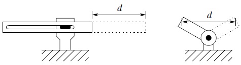
Figure 1.7 Linear vs. rotational link motion showing that a smaller revolute joint can cover the same distance d as a larger prismatic joint. The tip of a prismatic link can cover a distance equal to the length of the link. The tip of a rotational link of length a, by contrast, can cover a distance of 2a by rotating 180 degrees.
Thus, manipulators made from revolute joints occupy a smaller working volume than manipulators with linear axes. This increases the ability of the manipulator to work in the same space with other robots, machines, and people. At the same time, revolute-joint manipulators are better able to maneuver around obstacles and have a wider range of possible applications.
1.2.4 Wrists and End Effectors
The joints in the kinematic chain between the arm and end effector are referred to as the wrist. The wrist joints are nearly always all revolute. It is increasingly common to design manipulators with spherical wrists, by which we mean wrists whose three joint axes intersect at a common point, known as the wrist center point. Such a spherical wrist is shown in Figure 1.8.
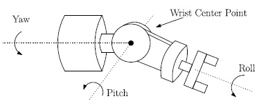
Figure 1.8 The spherical wrist. The axes of rotation of the spherical wrist are typically denoted roll, pitch, and yaw and intersect at a point called the wrist center point.
The spherical wrist greatly simplifies kinematic analysis, effectively allowing one to decouple the position and orientation of the end effector. Typically the manipulator will possess three DOF for position, which are produced by three or more joints in the arm. The number of DOF for orientation will then depend on the DOF of the wrist. It is common to find wrists having one, two, or three DOF depending on the application. For example, the SCARA robot shown in Figure 1.14 has four DOF: three for the arm, and one for the wrist, which has only a rotation about the final z-axis.
The arm and wrist assemblies of a robot are used primarily for positioning the hand, end effector, and any tool it may carry. It is the end effector or tool that actually performs the task. The simplest type of end effector is a gripper, such as shown in Figure 1.9, which is usually capable of only two actions, opening and closing. While this is adequate for materials transfer, some parts handling, or gripping simple tools, it is not adequate for other tasks such as welding, assembly, grinding, etc.
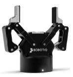
Figure 1.9 A two-finger gripper. (Photo courtesy of Robotiq, Inc.)
A great deal of research is therefore devoted to the design of special purpose end effectors as well as of tools that can be rapidly changed as the task dictates. Since we are concerned with the analysis and control of the manipulator itself and not in the particular application or end effector, we will not discuss the design of end effectors or the study of grasping and manipulation. There is also much research on the development of anthropomorphic hands such as that shown in Figure 1.10.

Figure 1.10 Anthropomorphic hand developed by Barrett Technologies. Such grippers allow for more dexterity and the ability to manipulate objects of various sizes and geometries. (Photo courtesy of Barrett Technologies.)
1.3 Common Kinematic Arrangements
There are many possible ways to construct kinematic chains using prismatic and revolute joints. However, in practice, only a few kinematic designs are commonly used. Here we briefly describe the most typical arrangements.
1.3.1 Articulated Manipulator (RRR)
The articulated manipulator is also called a revolute, elbow, or anthropomorphic manipulator. The KUKA 500 articulated arm is shown in Figure 1.11. In the anthropomorphic design the three links are designated as the body, upper arm, and forearm, respectively, as shown in Figure 1.11. The joint axes are designated as the waist (z0), shoulder (z1), and elbow (z2). Typically, the joint axis z2 is parallel to z1 and both z1 and z2 are perpendicular to z0. The workspace of the elbow manipulator is shown in Figure 1.12.
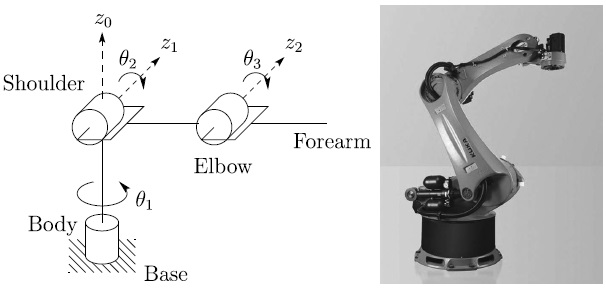
Figure 1.11 Symbolic representation of an RRR manipulator (left), and the KUKA 500 arm (right), which is a typical example of an RRR manipulator. The links and joints of the RRR configuration are analogous to human joints and limbs. (Photo courtesy of KUKA Robotics.)
Figure 1.12 Workspace of the elbow manipulator. The elbow manipulator provides a larger workspace than other kinematic designs relative to its size.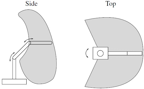
1.3.2 Spherical Manipulator (RRP)
By replacing the third joint, or elbow joint, in the revolute manipulator by a prismatic joint, one obtains the spherical manipulator shown in Figure 1.13. The term spherical manipulator derives from the fact that the joint coordinates coincide with the spherical coordinates of the end effector relative to a coordinate frame located at the shoulder joint. Figure 1.13 shows the Stanford Arm, one of the most well-known spherical robots.
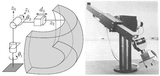
Figure 1.13 Schematic representation of an RRP manipulator, referred to as a spherical robot (left), and the Stanford Arm (right), an early example of a spherical arm. (Photo courtesy of the Coordinated Science Laboratory, University of Illinois at Urbana-Champaign.)
1.3.3 SCARA Manipulator (RRP)
The SCARA arm (for Selective Compliant Articulated Robot for Assembly) shown in Figure 1.14 is a popular manipulator, which, as its name suggests, is tailored for pick-and-place and assembly operations. Although the SCARA has an RRP structure, it is quite different from the spherical manipulator in both appearance and in its range of applications. Unlike the spherical design, which has z0 perpendicular to z1, and z1 perpendicular to z2, the SCARA has z0, z1, and z2 mutually parallel. Figure 1.14 shows the symbolic representation of a SCARA arm and the Yamaha YK-XC manipulator.

Figure 1.14 The ABB IRB910SC SCARA robot (left) and the symbolic representation showing a portion of its workspace (right). (Photo courtesy of ABB.)
1.3.4 Cylindrical Manipulator (RPP)
The cylindrical manipulator is shown in Figure 1.15. The first joint is revolute and produces a rotation about the base, while the second and third joints are prismatic. As the name suggests, the joint variables are the cylindrical coordinates of the end effector with respect to the base.
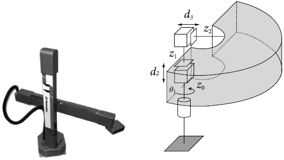
Figure 1.15 The ST Robotics R19 cylindrical robot (left) and the symbolic representation showing a portion of its workspace (right). Cylindrical robots are often used in materials transfer tasks. (Photo courtesy of ST Robotics.)
1.3.5 Cartesian Manipulator (PPP)
A manipulator whose first three joints are prismatic is known as a Cartesian manipulator. The joint variables of the Cartesian manipulator are the Cartesian coordinates of the end effector with respect to the base. As might be expected, the kinematic description of this manipulator is the simplest of all manipulators. Cartesian manipulators are useful for table-top assembly applications and, as gantry robots, for transfer of material or cargo. The symbolic representation of a Cartesian robot is shown in Figure 1.16.

Figure 1.16 The Yamaha YK-XC Cartesian robot (left) and the symbolic representation showing a portion of its workspace (right). Cartesian robots are often used in pick-and-place operations. (Photo courtesy of Yamaha Robotics.)
1.3.6 Parallel Manipulator
A parallel manipulator is one in which some subset of the links form a closed chain. More specifically, a parallel manipulator has two or more kinematic chains connecting the base to the end effector. Figure 1.17 shows the ABB IRB360 robot, which is a parallel manipulator. The closed-chain kinematics of parallel robots can result in greater structural rigidity, and hence greater accuracy, than open chain robots. The kinematic description of parallel robots is fundamentally different from that of serial link robots and therefore requires different methods of analysis.

Figure 1.17 The ABB IRB360 parallel robot. Parallel robots generally have higher structural rigidity than serial link robots. (Photo courtesy of ABB.)
1.4 Outline of the Text
The present textbook is divided into four parts. The first three parts are devoted to the study of manipulator arms. The final part treats the control of underactuated and mobile robots.
1.4.1 Manipulator Arms
We can use the simple example below to illustrate some of the major issues involved in the study of manipulator arms and to preview the topics covered. A typical application involving an industrial manipulator is shown in Figure 1.18. The manipulator is shown with a grinding tool that it must use to remove a certain amount of metal from a surface. Suppose we wish to move the manipulator from its home position to position A, from which point the robot is to follow the contour of the surface S to the point B, at constant velocity, while maintaining a prescribed force F normal to the surface. In so doing the robot will cut or grind the surface according to a predetermined specification. To accomplish this and even more general tasks, we must solve a number of problems. Below we give examples of these problems, all of which will be treated in more detail in the text.
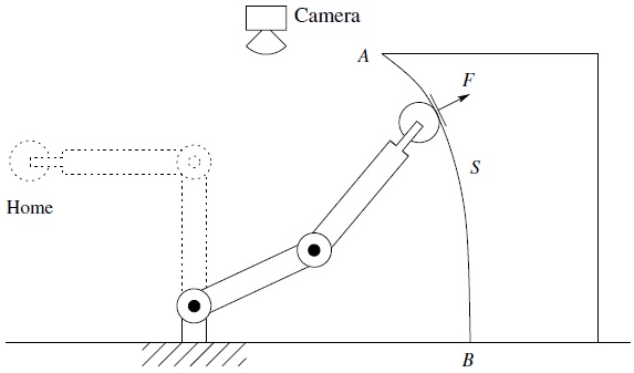
Figure 1.18 Two-link planar robot example. Each chapter of the text discusses a fundamental concept applicable to the task shown.
Chapter 2: Rigid Motions
The first problem encountered is to describe both the position of the tool and the locations A and B (and most likely the entire surface S) with respect to a common coordinate system. In Chapter 2 we describe representations of coordinate systems and transformations among various coordinate systems. We describe several ways to represent rotations and rotational transformations and we introduce so-called homogeneous transformations, which combine position and orientation into a single matrix representation.
Chapter 3: Forward Kinematics
Typically, the manipulator will be able to sense its own position in some manner using internal sensors (position encoders located at joints 1 and 2) that can measure directly the joint angles θ1 and θ2. We also need therefore to express the positions A and B in terms of these joint angles. This leads to the forward kinematics problem studied in Chapter 3, which is to determine the position and orientation of the end effector or tool in terms of the joint variables.
It is customary to establish a fixed coordinate system, called the world or base frame to which all objects including the manipulator are referenced. In this case we establish the base coordinate frame o0x0y0 at the base of the robot, as shown in Figure 1.19. The coordinates (x, y) of the tool are expressed in this coordinate frame as

Figure 1.19 Coordinate frames attached to the links of a two-link planar robot. Each coordinate frame moves as the corresponding link moves. The mathematical description of the robot motion is thus reduced to a mathematical description of moving coordinate frames.
in which a1 and a2 are the lengths of the two links, respectively. Also the orientation of the tool frame relative to the base frame is given by the direction cosines of the x2 and y2 axes relative to the x0 and y0 axes, that is,
which we may combine into a rotation matrix
Equations (1.1), (1.2), and (1.4) are called the forward kinematic equations for this arm. For a six-DOF robot these equations are quite complex and cannot be written down as easily as for the two-link manipulator. The general procedure that we discuss in Chapter 3 establishes coordinate frames at each joint and allows one to transform systematically among these frames using matrix transformations. The procedure that we use is referred to as the Denavit–Hartenberg convention. We then use homogeneous coordinates and homogeneous transformations, developed in Chapter 2, to simplify the transformation among coordinate frames.
Chapter 4: Velocity Kinematics
To follow a contour at constant velocity, or at any prescribed velocity, we must know the relationship between the tool velocity and the joint velocities. In this case we can differentiate Equations (1.1) and (1.2) to obtain
Using the vector notation ![]() and
and ![]() , we may write these equations as
, we may write these equations as
The matrix J defined by Equation (1.6) is called the Jacobian of the manipulator and is a fundamental object to determine for any manipulator. In Chapter 4 we present a systematic procedure for deriving the manipulator Jacobian.
The determination of the joint velocities from the end-effector velocities is conceptually simple since the velocity relationship is linear. Thus, the joint velocities are found from the end-effector velocities via the inverse Jacobian
where J− 1 is given by
The determinant of the Jacobian in Equation (1.6) is equal to a1a2sin θ2. Therefore, this Jacobian does not have an inverse when θ2 = 0 or θ2 = π, in which case the manipulator is said to be in a singular configuration, such as shown in Figure 1.20 for θ2 = 0. The determination of such singular configurations is important for several reasons. At singular configurations there are infinitesimal motions that are unachievable; that is, the manipulator end effector cannot move in certain directions. In the above example the end effector cannot move in the positive x2 direction when θ2 = 0. Singular configurations are also related to the nonuniqueness of solutions of the inverse kinematics. For example, for a given end-effector position of the two-link planar manipulator, there are in general two possible solutions to the inverse kinematics. Note that a singular configuration separates these two solutions in the sense that the manipulator cannot go from one to the other without passing through a singularity. For many applications it is important to plan manipulator motions in such a way that singular configurations are avoided.

Figure 1.20 A singular configuration results when the elbow is straight. In this configuration the two-link robot has only one DOF.
Chapter 5: Inverse Kinematics
Now, given the joint angles θ1, θ2 we can determine the end-effector coordinates x and y from Equations (1.1) and (1.2). In order to command the robot to move to location A we need the inverse; that is, we need to solve for the joint variables θ1, θ2 in terms of the x and y coordinates of A. This is the problem of inverse kinematics. Since the forward kinematic equations are nonlinear, a solution may not be easy to find, nor is there a unique solution in general. We can see in the case of a two-link planar mechanism that there may be no solution, for example if the given (x, y) coordinates are out of reach of the manipulator. If the given (x, y) coordinates are within the manipulator’s reach there may be two solutions as shown in Figure 1.21,

Figure 1.21 The two-link elbow robot has two solutions to the inverse kinematics except at singular configurations, the elbow up solution and the elbow down solution.
the so-called elbow up and elbow down configurations, or there may be exactly one solution if the manipulator must be fully extended to reach the point. There may even be an infinite number of solutions in some cases (Problem 1–19).
Consider the diagram of Figure 1.22. Using the law of cosines1 we see that the angle θ2 is given by
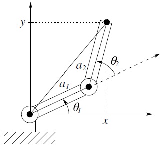
Figure 1.22 Solving for the joint angles of a two-link planar arm.
We could now determine θ2 as θ2 = cos − 1(D). However, a better way to find θ2 is to notice that if cos (θ2) is given by Equation (1.8), then sin (θ2) is given as
and, hence, θ2 can be found by
The advantage of this latter approach is that both the elbow-up and elbow-down solutions are recovered by choosing the negative and positive signs in Equation (1.10), respectively.
It is left as an exercise (Problem 1–17) to show that θ1 is now given as
Notice that the angle θ1 depends on θ2. This makes sense physically since we would expect to require a different value for θ1, depending on which solution is chosen for θ2.
Chapter 6: Dynamics
In Chapter 6 we develop techniques based on Lagrangian dynamics for systematically deriving the equations of motion for serial-link manipulators. Deriving the dynamic equations of motion for robots is not a simple task due to the large number of degrees of freedom and the nonlinearities present in the system. We also discuss the so-called recursive Newton–Euler method for deriving the robot equations of motion. The Newton–Euler formulation is well-suited for real-time computation for both simulation and control applications.
Chapter 7: Path Planning and Trajectory Generation
The robot control problem is typically decomposed hierarchically into three tasks: path planning, trajectory generation, and trajectory tracking. The path planning problem, considered in Chapter 7, is to determine a path in task space (or configuration space) to move the robot to a goal position while avoiding collisions with objects in its workspace. These paths encode position and orientation information without timing considerations, that is, without considering velocities and accelerations along the planned paths. The trajectory generation problem, also considered in Chapter 7, is to generate reference trajectories that determine the time history of the manipulator along a given path or between initial and final configurations. These are typically given in joint space as polynomial functions of time. We discuss the most common polynomial interpolation schemes used to generate these trajectories.
Chapter 8: Independent Joint Control
Once reference trajectories for the robot are specified, it is the task of the control system to track them. In Chapter 8 we discuss the motion control problem. We treat the twin problems of tracking and disturbance rejection, which are to determine the control inputs necessary to follow, or track, a reference trajectory, while simultaneously rejecting disturbances due to unmodeled dynamic effects such as friction and noise. We first model the actuator and drive-train dynamics and discuss the design of independent joint control algorithms.
A block diagram of a single-input/single-output (SISO) feedback control system is shown in Figure 1.23. We detail the standard approaches to robot control based on both frequency domain and state space techniques. We also introduce the notion of feedforward control for tracking time-varying trajectories. We also introduce the fundamental notion of computed torque, which is a feedforward disturbance cancellation scheme.
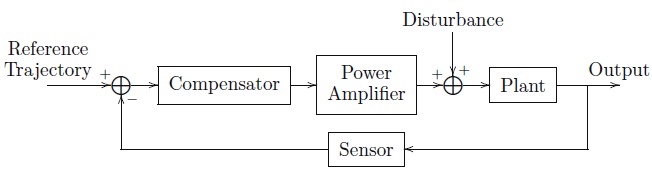
Figure 1.23 Basic structure of a feedback control system. The compensator measures the error between a reference and a measured output and produces a signal to the plant that is designed to drive the error to zero despite the presences of disturbances.
Chapter 9: Nonlinear and Multivariable Control
In Chapter 9 we discuss more advanced control techniques based on the Lagrangian dynamic equations of motion derived in Chapter 6. We introduce the notion of inverse dynamics control as a means for compensating the complex nonlinear interaction forces among the links of the manipulator. Robust and adaptive control of manipulators are also introduced using the direct method of Lyapunov and so-called passivity-based control.
Chapter 10: Force Control
In the example robot task above, once the manipulator has reached location A, it must follow the contour S maintaining a constant force normal to the surface. Conceivably, knowing the location of the object and the shape of the contour, one could carry out this task using position control alone. This would be quite difficult to accomplish in practice, however. Since the manipulator itself possesses high rigidity, any errors in position due to uncertainty in the exact location of the surface or tool would give rise to extremely large forces at the end effector that could damage the tool, the surface, or the robot. A better approach is to measure the forces of interaction directly and use a force control scheme to accomplish the task. In Chapter 10 we discuss force control and compliance, along with common approaches to force control, namely hybrid control and impedance control.
Chapter 11: Vision-Based Control
Cameras have become reliable and relatively inexpensive sensors in many robotic applications. Unlike joint sensors, which give information about the internal configuration of the robot, cameras can be used not only to measure the position of the robot but also to locate objects in the robot’s workspace. In Chapter 11 we discuss the use of computer vision to determine position and orientation of objects.
In some cases, we may wish to control the motion of the manipulator relative to some target as the end effector moves through free space. Here, force control cannot be used. Instead, we can use computer vision to close the control loop around the vision sensor. This is the topic of Chapter 11. There are several approaches to vision-based control, but we will focus on the method of Image-Based Visual Servo (IBVS). With IBVS, an error measured in image coordinates is directly mapped to a control input that governs the motion of the camera. This method has become very popular in recent years, and it relies on mathematical development analogous to that given in Chapter 4.
Chapter 12: Feedback Linearization
Chapter 12 discusses the method of nonlinear feedback linearization. Feedback linearization relies on more advanced tools from differential geometry. We discuss the Frobenius theorem, from which we prove necessary and sufficient conditions for a single-input nonlinear system to be equivalent under coordinate transformation and nonlinear feedback to a linear system. We apply the feedback linearization method to the control of elastic-joint robots, for which previous methods such as inverse dynamics cannot be applied.
1.4.2 Underactuated and Mobile Robots
Chapter 13: Underactuated Systems
Chapter 13 treats the control problem for underactuated robots, which have fewer actuators than degrees of freedom. Unlike the control of fully-actuated manipulators considered in Chapters 8–11, underactuated robots cannot track arbitrary trajectories and, consequently, the control problems are more challenging for this class of robots than for fully-actuated robots. We discuss the method of partial feedback linearization and introduce the notion of zero dynamics, which plays an important role in understanding how to control underactuated robots.
Chapter 14: Mobile Robots
Chapter 14 is devoted to the control of mobile robots, which are examples of so-called nonholonomic systems. We discuss controllability, stabilizability, and tracking control for this class of systems. Nonholonomic systems require the development of new tools for analysis and control, not treated in the previous chapters. We introduce the notions of chain-form systems, and differential flatness, which provide methods to transform nonholonomic systems into forms amenable to control design. We discuss two important results, Chow’s theorem and Brockett’s theorem, that can be used to determine when a nonholonomic system is controllable or stabilizable, respectively.
Problems
- What are the key features that distinguish robots from other forms of automation such as CNC milling machines?
- Briefly define each of the following terms: forward kinematics, inverse kinematics, trajectory planning, workspace, accuracy, repeatability, resolution, joint variable, spherical wrist, end effector.
- What are the main ways to classify robots?
- Make a list of 10 robot applications. For each application discuss which type of manipulator would be best suited; which least suited. Justify your choices in each case.
- List several applications for nonservo robots; for point-to-point robots; for continuous path robots.
- List five applications that a continuous path robot could do that a point-to-point robot could not do.
- List five applications for which computer vision would be useful in robotics.
- List five applications for which either tactile sensing or force feedback control would be useful in robotics.
- Suppose we could close every factory today and reopen them tomorrow fully automated with robots. What would be some of the economic and social consequences of such a development?
- Suppose a law were passed banning all future use of industrial robots. What would be some of the economic and social consequences of such an act?
- Discuss applications for which redundant manipulators would be useful.
- Referring to Figure 1.24, suppose that the tip of a single link travels a distance d between two points. A linear axis would travel the distance d while a rotational link would travel through an arc length ℓθ as shown. Using the law of cosines, show that the distance d is given by
which is of course less than ℓθ. With 10-bit accuracy, ℓ = 1 meter, and θ = 90°, what is the resolution of the linear link? of the rotational link?
- For the single-link revolute arm shown in Figure 1.24, if the length of the link is 50 cm and the arm travels 180 degrees, what is the control resolution obtained with an 8-bit encoder?
- Repeat Problem 1–13 assuming that the 8-bit encoder is located on the motor shaft that is connected to the link through a 50:1 gear reduction. Assume perfect gears.
- Why is accuracy generally less than repeatability?
- How could manipulator accuracy be improved using endpoint sensing? What difficulties might endpoint sensing introduce into the control problem?
- Derive Equation (1.11).
- For the two-link manipulator of Figure 1.19 suppose a1 = a2 = 1.
- Find the coordinates of the tool when
 and
and  .
. -
If the joint velocities are constant at
 ,
,  , what is the velocity of the tool? What is the instantaneous tool velocity when
  ?
? - Write a computer program to plot the joint angles as a function of time given the tool locations and velocities as a function of time in Cartesian coordinates.
- Suppose we desire that the tool follow a straight line between the points (0,2) and (2,0) at constant speed s. Plot the time history of joint angles.
- Find the coordinates of the tool when
- For the two-link planar manipulator of Figure 1.19 is it possible for there to be an infinite number of solutions to the inverse kinematic equations? If so, explain how this can occur.
- Explain why it might be desirable to reduce the mass of distal links in a manipulator design. List some ways this can be done. Discuss any possible disadvantages of such designs.
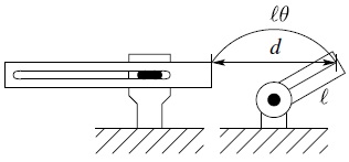
Figure 1.24 Diagram for Problem 1–12, 1–13, and 1–14.
Notes and References
We give below some of the important milestones in the history of modern robotics.
- 1947 — The first servoed electric powered teleoperator is developed.
- 1948 — A teleoperator is developed incorporating force feedback.
- 1949 — Research on numerically controlled milling machine is initiated.
- 1954 — George Devol designs the first programmable robot
- 1956 — Joseph Engelberger, a Columbia University physics student, buys the rights to Devol’s robot and founds the Unimation Company.
- 1961 — The first Unimate robot is installed in a Trenton, New Jersey plant of General Motors to tend a die casting machine.
- 1961 — The first robot incorporating force feedback is developed.
- 1963 — The first robot vision system is developed.
- 1971 — The Stanford Arm is developed at Stanford University.
- 1973 — The first robot programming language (WAVE) is developed at Stanford.
- 1974 — Cincinnati Milacron introduced the T3 robot with computer control.
- 1975 — Unimation Inc. registers its first financial profit.
- 1976 — The Remote Center Compliance (RCC) device for part insertion in assembly is developed at Draper Labs in Boston.
- 1976 — Robot arms are used on the Viking I and II space probes and land on Mars.
- 1978 — Unimation introduces the PUMA robot, based on designs from a General Motors study.
- 1979 — The SCARA robot design is introduced in Japan.
- 1981 — The first direct-drive robot is developed at Carnegie-Mellon University.
- 1982 — Fanuc of Japan and General Motors form GM Fanuc to market robots in North America.
- 1983 — Adept Technology is founded and successfully markets the direct-drive robot.
- 1986 — The underwater robot, Jason, of the Woods Hole Oceanographic Institute, explores the wreck of the Titanic, found a year earlier by Dr. Robert Barnard.
- 1988 — Stäubli Group purchases Unimation from Westinghouse.
- 1988 — The IEEE Robotics and Automation Society is formed.
- 1993 — The experimental robot, ROTEX, of the German Aerospace Agency (DLR) was flown aboard the space shuttle Columbia and performed a variety of tasks under both teleoperated and sensor-based offline programmed modes.
- 1996 — Honda unveils its Humanoid robot; a project begun in secret in 1986.
- 1997 — The first robot soccer competition, RoboCup-97, is held in Nagoya, Japan and draws 40 teams from around the world.
- 1997 — The Sojourner mobile robot travels to Mars aboard NASA’s Mars PathFinder mission.
- 2001 — Sony begins to mass produce the first household robot, a robot dog named Aibo.
- 2001 — The Space Station Remote Manipulation System (SSRMS) is launched in space on board the space shuttle Endeavor to facilitate continued construction of the space station.
- 2001 — The first telesurgery is performed when surgeons in New York perform a laparoscopic gall bladder removal on a woman in Strasbourg, France.
- 2001 — Robots are used to search for victims at the World Trade Center site after the September 11th tragedy.
- 2002 — Honda’s Humanoid Robot ASIMO rings the opening bell at the New York Stock Exchange on February 15th.
- 2004 — The Mars rovers Spirit and Opportunity both landed on the surface of Mars in January of this year. Both rovers far outlived their planned missions of 90 Martian days. Spirit was active until 2010 and Opportunity stayed active until 2018, and holds the record for having driven farther than any off-Earth vehicle in history.
- 2005 — ROKVISS (Robotic Component Verification on board the International Space Station), the experimental teleoperated arm built by the German Aerospace Center (DLR), undergoes its first tests in space.
- 2005 — Boston Dynamics releases the quadrupedal robot Big Dog.
- 2007 — Willow Garage develops the Robot Operating System (ROS).
- 2011 — Robonaut 2 was launched to the International Space Station.
- 2017 — A robot called Sophia was granted Saudi Arabian citizenship, becoming the first robot ever to have a nationality.
Note
- 1 See Appendix A.