CHAPTER 2
RIGID MOTIONS
A large part of robot kinematics is concerned with establishing various coordinate frames to represent the positions and orientations of rigid objects, and with transformations among these coordinate frames. Indeed, the geometry of three-dimensional space and of rigid motions plays a central role in all aspects of robotic manipulation. In this chapter we study the operations of rotation and translation, and introduce the notion of homogeneous transformations.
Homogeneous transformations combine the operations of rotation and translation into a single matrix multiplication, and are used in Chapter 3 to derive the so-called forward kinematic equations of rigid manipulators. Since we make extensive use of elementary matrix theory, the reader may wish to review Appendix B before beginning this chapter.
We begin by examining representations of points and vectors in a Euclidean space equipped with multiple coordinate frames. Following this, we introduce the concept of a rotation matrix to represent relative orientations among coordinate frames. We then combine these two concepts to build homogeneous transformation matrices, which can be used to simultaneously represent the position and orientation of one coordinate frame relative to another. Furthermore, homogeneous transformation matrices can be used to perform coordinate transformations. Such transformations allow us to represent various quantities in different coordinate frames, a facility that we will often exploit in subsequent chapters.
2.1 Representing Positions
Before developing representation schemes for points and vectors, it is instructive to distinguish between the two fundamental approaches to geometric reasoning: the synthetic approach and the analytic approach. In the former, one reasons directly about geometric entities (e.g., points or lines), while in the latter, one represents these entities using coordinates or equations, and reasoning is performed via algebraic manipulations. The latter approach requires the choice of a reference coordinate frame. A coordinate frame consists of an origin (a single point in space), and two or three orthogonal coordinate axes, for two- and three-dimensional spaces, respectively.
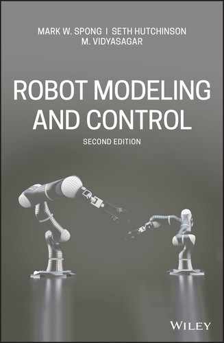
Consider Figure 2.1, which shows two coordinate frames that differ in orientation by an angle of 45°. Using the synthetic approach, without ever assigning coordinates to points or vectors, one can say that x0 is perpendicular to y0, or that v1 × v2 defines a vector that is perpendicular to the plane containing v1 and v2, in this case pointing out of the page.
Figure 2.1 Two coordinate frames, a point p, and two vectors v1 and v2.
In robotics, one typically uses analytic reasoning, since robot tasks are often defined using Cartesian coordinates. Of course, in order to assign coordinates it is necessary to specify a reference coordinate frame. Consider again Figure 2.1. We could specify the coordinates of the point p with respect to either frame o0x0y0 or frame o1x1y1. In the former case we might assign to p the coordinate vector (5, 6) and in the latter case ( − 3, 3). So that the reference frame will always be clear, we will adopt a notation in which a superscript is used to denote the reference frame. Thus, we write
Geometrically, a point corresponds to a specific location in space. We stress here that p is a geometric entity, a point in space, while both ![]() and
and ![]() are coordinate vectors that represent the location of this point in space with respect to coordinate frames o0x0y0 and o1x1y1, respectively. When no confusion can arise, we may simply refer to these coordinate frames as frame 0 and frame 1, respectively.
are coordinate vectors that represent the location of this point in space with respect to coordinate frames o0x0y0 and o1x1y1, respectively. When no confusion can arise, we may simply refer to these coordinate frames as frame 0 and frame 1, respectively.
Since the origin of a coordinate frame is also a point in space, we can assign coordinates that represent the position of the origin of one coordinate frame with respect to another. In Figure 2.1, for example, we may have
Thus, o01 specifies the coordinates of the point o1 relative to frame 0 and o10 specifies the coordinates of the point 00 relative to frame 1. In cases where there is only a single coordinate frame, or in which the reference frame is obvious, we will often omit the superscript. This is a slight abuse of notation, and the reader is advised to bear in mind the difference between the geometric entity called p and any particular coordinate vector that is assigned to represent p. The former is independent of the choice of coordinate frames, while the latter obviously depends on the choice of coordinate frames.
While a point corresponds to a specific location in space, a vector specifies a direction and a magnitude. Vectors can be used, for example, to represent displacements or forces. Therefore, while the point p is not equivalent to the vector v1, the displacement from the origin o0 to the point p is given by the vector v1. In this text, we will use the term vector to refer to what are sometimes called free vectors, that is, vectors that are not constrained to be located at a particular point in space. Under this convention, it is clear that points and vectors are not equivalent, since points refer to specific locations in space, but a free vector can be moved to any location in space. Thus, two vectors are equal if they have the same direction and the same magnitude.
When assigning coordinates to vectors, we use the same notational convention that we used when assigning coordinates to points. Thus, v1 and v2 are geometric entities that are invariant with respect to the choice of coordinate frames, but the representation by coordinates of these vectors depends directly on the choice of reference coordinate frame. In the example of Figure 2.1, we would obtain
In order to perform algebraic manipulations using coordinates, it is essential that all coordinate vectors be defined with respect to the same coordinate frame. In the case of free vectors, it is enough that they be defined with respect to “parallel” coordinate frames, that is, frames whose respective coordinate axes are parallel, since only their magnitude and direction are specified and not their absolute locations in space.
Using this convention, an expression of the form ![]() , where
, where ![]() and
and ![]() are as in Figure 2.1, is not defined since the frames o0x0y0 and o1x1y1 are not parallel. Thus, we see a clear need not only for a representation system that allows points to be expressed with respect to various coordinate frames, but also for a mechanism that allows us to transform the coordinates of points from one coordinate frame to another. Such coordinate transformations are the topic for much of the remainder of this chapter.
are as in Figure 2.1, is not defined since the frames o0x0y0 and o1x1y1 are not parallel. Thus, we see a clear need not only for a representation system that allows points to be expressed with respect to various coordinate frames, but also for a mechanism that allows us to transform the coordinates of points from one coordinate frame to another. Such coordinate transformations are the topic for much of the remainder of this chapter.
2.2 Representing Rotations
In order to represent the relative position and orientation of one rigid body with respect to another, we attach coordinate frames to each body, and then specify the geometric relationship between these coordinate frames. In Section 2.1 we saw how one can represent the position of the origin of one frame with respect to another frame. In this section, we address the problem of describing the orientation of one coordinate frame relative to another frame. We begin with the case of rotations in the plane, and then generalize our results to the case of rotations in a three-dimensional space.
2.2.1 Rotation in the Plane
Figure 2.2 shows two coordinate frames, with frame o1x1y1 obtained by rotating frame o0x0y0 by an angle θ. Perhaps the most obvious way to represent the relative orientation of these two frames is merely to specify the angle of rotation θ. There are two immediate disadvantages to such a representation. First, there is a discontinuity in the mapping from relative orientation to the value of θ in a neighborhood of θ = 0. In particular, for θ = 2π − ε, small changes in orientation can produce large changes in the value of θ, for example, a rotation by ε causes θ to “wrap around” to zero. Second, this choice of representation does not scale well to the three-dimensional case.

Figure 2.2 Coordinate frame o1x1y1 is oriented at an angle θ with respect to o0x0y0.
A slightly less obvious way to specify the orientation is to specify the coordinate vectors for the axes of frame o1x1y1 with respect to coordinate frame o0x0y0:
in which ![]() and
and ![]() are the coordinates in frame o0x0y0 of unit vectors x1 and y1, respectively.1
A matrix in this form is called a rotation matrix. Rotation matrices have a number of special properties that we will discuss below.
are the coordinates in frame o0x0y0 of unit vectors x1 and y1, respectively.1
A matrix in this form is called a rotation matrix. Rotation matrices have a number of special properties that we will discuss below.
In the two-dimensional case, it is straightforward to compute the entries of this matrix. As illustrated in Figure 2.2,
which gives
Note that we have continued to use the notational convention of allowing the superscript to denote the reference frame. Thus, ![]() is a matrix whose column vectors are the coordinates of the unit vectors along the axes of frame o1x1y1 expressed relative to frame o0x0y0.
is a matrix whose column vectors are the coordinates of the unit vectors along the axes of frame o1x1y1 expressed relative to frame o0x0y0.
Although we have derived the entries for ![]() in terms of the angle θ, it is not necessary that we do so. An alternative approach, and one that scales nicely to the three-dimensional case, is to build the rotation matrix by projecting the axes of frame o1x1y1 onto the coordinate axes of frame o0x0y0. Recalling that the dot product of two unit vectors gives the projection of one onto the other, we obtain
in terms of the angle θ, it is not necessary that we do so. An alternative approach, and one that scales nicely to the three-dimensional case, is to build the rotation matrix by projecting the axes of frame o1x1y1 onto the coordinate axes of frame o0x0y0. Recalling that the dot product of two unit vectors gives the projection of one onto the other, we obtain
which can be combined to obtain the rotation matrix
Thus, the columns of ![]() specify the direction cosines of the coordinate axes of o1x1y1 relative to the coordinate axes of o0x0y0. For example, the first column (x1 · x0, x1 · y0) of
specify the direction cosines of the coordinate axes of o1x1y1 relative to the coordinate axes of o0x0y0. For example, the first column (x1 · x0, x1 · y0) of ![]() specifies the direction of x1 relative to the frame o0x0y0. Note that the right-hand sides of these equations are defined in terms of geometric entities, and not in terms of their coordinates. Examining Figure 2.2 it can be seen that this method of defining the rotation matrix by projection gives the same result as we obtained in Equation (2.1).
specifies the direction of x1 relative to the frame o0x0y0. Note that the right-hand sides of these equations are defined in terms of geometric entities, and not in terms of their coordinates. Examining Figure 2.2 it can be seen that this method of defining the rotation matrix by projection gives the same result as we obtained in Equation (2.1).
If we desired instead to describe the orientation of frame o0x0y0 with respect to the frame o1x1y1 (that is, if we desired to use the frame o1x1y1 as the reference frame), we would construct a rotation matrix of the form
Since the dot product is commutative, (that is, xi · yj = yj · xi), we see that
In a geometric sense, the orientation of o0x0y0 with respect to the frame o1x1y1 is the inverse of the orientation of o1x1y1 with respect to the frame o0x0y0. Algebraically, using the fact that coordinate axes are mutually orthogonal, it can readily be seen that
The above relationship implies that ![]() and it is easily shown that the column vectors of
and it is easily shown that the column vectors of ![]() are of unit length and mutually orthogonal (Problem 2–4). Thus
are of unit length and mutually orthogonal (Problem 2–4). Thus ![]() is an orthogonal matrix. It also follows from the above that (Problem 2–5)
is an orthogonal matrix. It also follows from the above that (Problem 2–5) ![]() . If we restrict ourselves to right-handed coordinate frames, as defined in Appendix B, then
. If we restrict ourselves to right-handed coordinate frames, as defined in Appendix B, then ![]() (Problem 2–5).
(Problem 2–5).
More generally, these properties extend to higher dimensions, which can be formalized as the so-called special orthogonal group of order n.
Definition 2.1.
The special orthogonal group of order n, denoted SO(n), is the set of n × n real-valued matrices
Thus, for any ![]() the following properties hold
the following properties hold

- The columns (and therefore the rows) of
 are mutually orthogonal
 - Each column (and therefore each row) of
 is a unit vector
The special case, SO(2), respectively, SO(3), is called the rotation group of order 2, respectively 3.
To provide further geometric intuition for the notion of the inverse of a rotation matrix, note that in the two-dimensional case, the inverse of the rotation matrix corresponding to a rotation by angle θ can also be easily computed simply by constructing the rotation matrix for a rotation by the angle − θ:
2.2.2 Rotations in Three Dimensions
The projection technique described above scales nicely to the three-dimensional case. In three dimensions, each axis of the frame o1x1y1z1 is projected onto coordinate frame o0x0y0z0. The resulting rotation matrix R ∈ SO(3) is given by
As was the case for rotation matrices in two dimensions, matrices in this form are orthogonal, with determinant equal to 1 and therefore elements of SO(3).
Example 2.1.
Suppose the frame o1x1y1z1 is rotated through an angle θ about the z0-axis, and we wish to find the resulting transformation matrix ![]() . By convention, the right hand rule (see Appendix B) defines the positive sense for the angle θ to be such that rotation by θ about the z-axis would advance a right-hand threaded screw along the positive z-axis.
. By convention, the right hand rule (see Appendix B) defines the positive sense for the angle θ to be such that rotation by θ about the z-axis would advance a right-hand threaded screw along the positive z-axis.
From Figure 2.3 we see that
and
while all other dot products are zero. Thus, the rotation matrix ![]() has a particularly simple form in this case, namely
has a particularly simple form in this case, namely

Figure 2.3 Rotation about z0 by an angle θ.
The rotation matrix given in Equation (2.3) is called a basic rotation matrix (about the z-axis). In this case we find it useful to use the more descriptive notation ![]() instead of
instead of ![]() to denote the matrix. It is easy to verify that the basic rotation matrix
to denote the matrix. It is easy to verify that the basic rotation matrix ![]() has the properties
has the properties
which together imply
Similarly, the basic rotation matrices representing rotations about the x and y-axes are given as (Problem 2–8)

which also satisfy properties analogous to Equations (2.4)–(2.6).
Example 2.2.
Consider the frames o0x0y0z0 and o1x1y1z1 shown in Figure 2.4.
Projecting the unit vectors x1, y1, z1 onto x0, y0, z0 gives the coordinates of x1, y1, z1 in the o0x0y0z0 frame as

The rotation matrix ![]() specifying the orientation of o1x1y1z1 relative to o0x0y0z0 has these as its column vectors, that is,
specifying the orientation of o1x1y1z1 relative to o0x0y0z0 has these as its column vectors, that is,
Figure 2.4 Defining the relative orientation of two frames.
2.3 Rotational Transformations
Figure 2.5 shows a rigid object S to which a coordinate frame o1x1y1z1 is attached. Given the coordinates ![]() of the point p (in other words, given the coordinates of p with respect to the frame o1x1y1z1), we wish to determine the coordinates of p relative to a fixed reference frame o0x0y0z0. The coordinates
of the point p (in other words, given the coordinates of p with respect to the frame o1x1y1z1), we wish to determine the coordinates of p relative to a fixed reference frame o0x0y0z0. The coordinates ![]() satisfy the equation
satisfy the equation

Figure 2.5 Coordinate frame attached to a rigid body.
In a similar way, we can obtain an expression for the coordinates ![]() by projecting the point p onto the coordinate axes of the frame o0x0y0z0, giving
by projecting the point p onto the coordinate axes of the frame o0x0y0z0, giving

Combining these two equations we obtain

But the matrix in this final equation is merely the rotation matrix ![]() , which leads to
, which leads to
Thus, the rotation matrix ![]() can be used not only to represent the orientation of coordinate frame o1x1y1z1 with respect to frame o0x0y0z0, but also to transform the coordinates of a point from one frame to another. If a given point is expressed relative to o1x1y1z1 by coordinates
can be used not only to represent the orientation of coordinate frame o1x1y1z1 with respect to frame o0x0y0z0, but also to transform the coordinates of a point from one frame to another. If a given point is expressed relative to o1x1y1z1 by coordinates ![]() , then
, then ![]() represents the same point
expressed relative to the frame o0x0y0z0.
represents the same point
expressed relative to the frame o0x0y0z0.
We can also use rotation matrices to represent rigid motions that correspond to pure rotation. For example, in Figure 2.6(a) one corner of the block is located at the point pa in space. Figure 2.6(b) shows the same block after it has been rotated about z0 by the angle π. The same corner of the block is now located at point pb in space. It is possible to derive the coordinates for pb given only the coordinates for pa and the rotation matrix that corresponds to the rotation about z0. To see how this can be accomplished, imagine that a coordinate frame is rigidly attached to the block in Figure 2.6(a), such that it is coincident with the frame o0x0y0z0. After the rotation by π, the block’s coordinate frame, which is rigidly attached to the block, is also rotated by π. If we denote this rotated frame by o1x1y1z1, we obtain
In the local coordinate frame o1x1y1z1, the point pb has the coordinate representation ![]() . To obtain its coordinates with respect to frame o0x0y0z0, we merely apply the coordinate transformation Equation (2.9), giving
. To obtain its coordinates with respect to frame o0x0y0z0, we merely apply the coordinate transformation Equation (2.9), giving
It is important to notice that the local coordinates ![]() of the corner of the block do not change as the block rotates, since they are defined in terms of the block’s own coordinate frame. Therefore, when the block’s frame is aligned with the reference frame o0x0y0z0 (that is, before the rotation is performed), the coordinates
of the corner of the block do not change as the block rotates, since they are defined in terms of the block’s own coordinate frame. Therefore, when the block’s frame is aligned with the reference frame o0x0y0z0 (that is, before the rotation is performed), the coordinates ![]() equals
equals ![]() , since before the rotation is performed, the point pa is coincident with the corner of the block. Therefore, we can substitute
, since before the rotation is performed, the point pa is coincident with the corner of the block. Therefore, we can substitute ![]() into the previous equation to obtain
into the previous equation to obtain
This equation shows how to use a rotation matrix to represent a rotational motion. In particular, if the point pb is obtained by rotating the point pa as defined by the rotation matrix ![]() , then the coordinates of pb with respect to the reference frame are given by
, then the coordinates of pb with respect to the reference frame are given by
This same approach can be used to rotate vectors with respect to a coordinate frame, as the following example illustrates.
Example 2.3.
The vector v with coordinates v0 = (0, 1, 1) is rotated about y0 by ![]() as shown in Figure 2.7. The resulting vector v1 is given by
as shown in Figure 2.7. The resulting vector v1 is given by
Thus, a third interpretation of a rotation matrix ![]() is as an operator acting on vectors in a fixed frame. In other words, instead of relating the coordinates of a fixed vector with respect to two different coordinate frames, Equation (2.10) can represent the coordinates in o0x0y0z0 of a vector v1 that is obtained from a vector v by a given rotation.
is as an operator acting on vectors in a fixed frame. In other words, instead of relating the coordinates of a fixed vector with respect to two different coordinate frames, Equation (2.10) can represent the coordinates in o0x0y0z0 of a vector v1 that is obtained from a vector v by a given rotation.
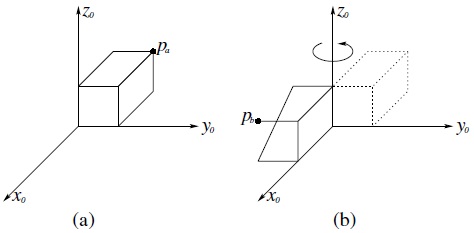
Figure 2.6 The block in (b) is obtained by rotating the block in (a) by π about z0.
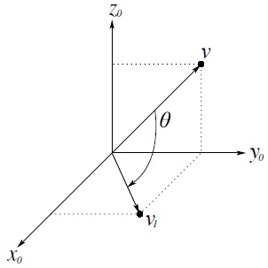
Figure 2.7 Rotating a vector about axis y0.
As we have seen, rotation matrices can serve several roles. A rotation matrix, either ![]() or
or ![]() , can be interpreted in three distinct ways:
, can be interpreted in three distinct ways:
- It represents a coordinate transformation relating the coordinates of a point p in two different frames.
- It gives the orientation of a transformed coordinate frame with respect to a fixed coordinate frame.
- It is an operator taking a vector and rotating it to give a new vector in the same coordinate frame.
The particular interpretation of a given rotation matrix ![]() should be made clear by the context.
should be made clear by the context.
Similarity Transformations
A coordinate frame is defined by a set of basis vectors, for example, unit vectors along the three coordinate axes. This means that a rotation matrix, as a coordinate transformation, can also be viewed as defining a change of basis from one frame to another. The matrix representation of a general linear transformation is transformed from one frame to another using a so-called similarity transformation. For example, if A is the matrix representation of a given linear transformation in o0x0y0z0 and B is the representation of the same linear transformation in o1x1y1z1 then A and B are related as
where ![]() is the coordinate transformation between frames o1x1y1z1 and o0x0y0z0. In particular, if A itself is a rotation, then so is B, and thus the use of similarity transformations allows us to express the same rotation easily with respect to different frames.
is the coordinate transformation between frames o1x1y1z1 and o0x0y0z0. In particular, if A itself is a rotation, then so is B, and thus the use of similarity transformations allows us to express the same rotation easily with respect to different frames.
Example 2.4.
Henceforth, whenever convenient we use the shorthand notation cθ = cos θ, sθ = sin θ for trigonometric functions. Suppose frames o0x0y0z0 and o1x1y1z1 are related by the rotation

If A = Rz, θ relative to the frame o0x0y0z0, then, relative to frame o1x1y1z1 we have
In other words, B is a rotation about the z0-axis but expressed relative to the frame o1x1y1z1. This notion will be useful below and in later sections.
2.4 Composition of Rotations
In this section we discuss the composition of rotations. It is important for subsequent chapters that the reader understand the material in this section thoroughly before moving on.
2.4.1 Rotation with Respect to the Current Frame
Recall that the matrix ![]() in Equation (2.9) represents a rotational transformation between the frames o0x0y0z0 and o1x1y1z1. Suppose we now add a third coordinate frame o2x2y2z2 related to the frames o0x0y0z0 and o1x1y1z1 by rotational transformations. A given point p can then be represented by coordinates specified with respect to any of these three frames:
in Equation (2.9) represents a rotational transformation between the frames o0x0y0z0 and o1x1y1z1. Suppose we now add a third coordinate frame o2x2y2z2 related to the frames o0x0y0z0 and o1x1y1z1 by rotational transformations. A given point p can then be represented by coordinates specified with respect to any of these three frames: ![]() ,
, ![]() , and
, and ![]() The relationship among these representations of p is
The relationship among these representations of p is
where each ![]() is a rotation matrix. Substituting Equation (2.14) into Equation (2.13) gives
is a rotation matrix. Substituting Equation (2.14) into Equation (2.13) gives
Note that ![]() and
and ![]() represent rotations relative to the frame o0x0y0z0 while
represent rotations relative to the frame o0x0y0z0 while ![]() represents a rotation relative to the frame o1x1y1z1. Comparing Equations (2.15) and (2.16) we can immediately infer
represents a rotation relative to the frame o1x1y1z1. Comparing Equations (2.15) and (2.16) we can immediately infer
Equation (2.17) is the composition law for rotational transformations. It states that, in order to transform the coordinates of a point p from its representation ![]() in the frame o2x2y2z2 to its representation
in the frame o2x2y2z2 to its representation ![]() in the frame o0x0y0z0, we may first transform to its coordinates
in the frame o0x0y0z0, we may first transform to its coordinates ![]() in the frame o1x1y1z1 using
in the frame o1x1y1z1 using ![]() and then transform
and then transform ![]() to
to ![]() using
using ![]() .
.
We may also interpret Equation (2.17) as follows. Suppose that initially all three of the coordinate frames coincide. We first rotate the frame o1x1y1z1 relative to o0x0y0z0 according to the transformation ![]() . Then, with the frames o1x1y1z1 and o2x2y2z2 coincident, we rotate o2x2y2z2 relative to o1x1y1z1 according to the transformation
. Then, with the frames o1x1y1z1 and o2x2y2z2 coincident, we rotate o2x2y2z2 relative to o1x1y1z1 according to the transformation ![]() . The resulting frame, o2x2y2z2 has orientation with respect to o0x0y0z0 given by
. The resulting frame, o2x2y2z2 has orientation with respect to o0x0y0z0 given by ![]() . We call the frame relative to which the rotation occurs the current frame.
. We call the frame relative to which the rotation occurs the current frame.
Example 2.5.
Suppose a rotation matrix ![]() represents a rotation of angle ϕ about the current y-axis followed by a rotation of angle θ about the current z-axis as shown in Figure 2.8. Then the matrix
represents a rotation of angle ϕ about the current y-axis followed by a rotation of angle θ about the current z-axis as shown in Figure 2.8. Then the matrix ![]() is given by
is given by
Figure 2.8 Composition of rotations about current axes.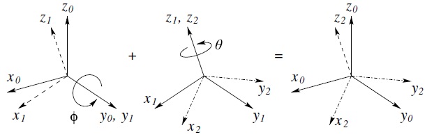
It is important to remember that the order in which a sequence of rotations is performed, and consequently the order in which the rotation matrices are multiplied together, is crucial. The reason is that rotation, unlike position, is not a vector quantity and so rotational transformations do not commute in general.
Example 2.6.
Suppose that the above rotations are performed in the reverse order, that is, first a rotation about the current z-axis followed by a rotation about the current y-axis. Then the resulting rotation matrix is given by

2.4.2 Rotation with Respect to the Fixed Frame
Many times it is desired to perform a sequence of rotations, each about a given fixed coordinate frame, rather than about successive current frames. For example we may wish to perform a rotation about x0 followed by a rotation about y0 (and not y1!). We will refer to o0x0y0z0 as the fixed frame. In this case the composition law given by Equation (2.17) is not valid. It turns out that the correct composition law in this case is simply to multiply the successive rotation matrices in the reverse order from that given by Equation (2.17). Note that the rotations themselves are not performed in reverse order. Rather they are performed about the fixed frame instead of about the current frame.
To see this, suppose we have two frames o0x0y0z0 and o1x1y1z1 related by the rotational transformation ![]() . If R ∈ SO(3) represents a rotation relative to o0x0y0z0, we know from Section 2.3 that the representation for R in the current frame o1x1y1z1 is given by (
. If R ∈ SO(3) represents a rotation relative to o0x0y0z0, we know from Section 2.3 that the representation for R in the current frame o1x1y1z1 is given by (![]() . Therefore, applying the composition law for rotations about the current axis yields
. Therefore, applying the composition law for rotations about the current axis yields
Thus, when a rotation ![]() is performed with respect to the world coordinate frame, the current rotation matrix is premultiplied by
is performed with respect to the world coordinate frame, the current rotation matrix is premultiplied by ![]() to obtain the desired rotation matrix.
to obtain the desired rotation matrix.
Example 2.7. (Rotations about Fixed Axes)
Referring to Figure 2.9, suppose that a rotation matrix ![]() represents a rotation of angle ϕ about y0 followed by a rotation of angle θ about the fixed z0. The second rotation about the fixed axis is given by
represents a rotation of angle ϕ about y0 followed by a rotation of angle θ about the fixed z0. The second rotation about the fixed axis is given by ![]() , which is the basic rotation about the z-axis expressed relative to the frame o1x1y1z1 using a similarity transformation. Therefore, the composition rule for rotational transformations gives us
, which is the basic rotation about the z-axis expressed relative to the frame o1x1y1z1 using a similarity transformation. Therefore, the composition rule for rotational transformations gives us
It is not necessary to remember the above derivation, only to note by comparing Equation (2.21) with Equation (2.18) that we obtain the same basic rotation matrices, but in the reverse order.
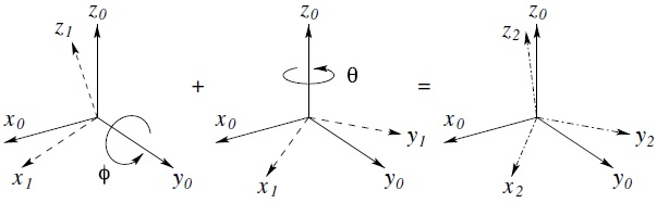
Figure 2.9 Composition of rotations about fixed axes.
2.4.3 Rules for Composition of Rotations
We can summarize the rule of composition of rotational transformations by the following recipe. Given a fixed frame o0x0y0z0 and a current frame o1x1y1z1, together with rotation matrix ![]() relating them, if a third frame o2x2y2z2 is obtained by a rotation
relating them, if a third frame o2x2y2z2 is obtained by a rotation ![]() performed relative to the current frame then postmultiply
performed relative to the current frame then postmultiply ![]() by
by ![]() to obtain
to obtain
If the second rotation is to be performed relative to the fixed frame then it is both confusing and inappropriate to use the notation ![]() to represent this rotation. Therefore, if we represent the rotation by
to represent this rotation. Therefore, if we represent the rotation by ![]() , we premultiply
, we premultiply ![]() by
by ![]() to obtain
to obtain
In each case ![]() represents the transformation between the frames o0x0y0z0 and o2x2y2z2. The frame o2x2y2z2 that results from Equation (2.22) will be different from that resulting from Equation (2.23).
represents the transformation between the frames o0x0y0z0 and o2x2y2z2. The frame o2x2y2z2 that results from Equation (2.22) will be different from that resulting from Equation (2.23).
Using the above rule for composition of rotations, it is an easy matter to determine the result of multiple sequential rotational transformations.
Example 2.8.
Suppose R is defined by the following sequence of basic rotations in the order specified:
- A rotation of θ about the current x-axis
- A rotation of ϕ about the current z-axis
- A rotation of α about the fixed z-axis
- A rotation of β about the current y-axis
- A rotation of δ about the fixed x-axis
In order to determine the cumulative effect of these rotations we simply begin with the first rotation Rx, θ and pre- or postmultiply as the case may be to obtain
2.5 Parameterizations of Rotations
The nine elements rij in a general rotational transformation ![]() are not independent quantities. Indeed, a rigid body possesses at most three rotational degrees of freedom, and thus at most three quantities are required to specify its orientation. This can be easily seen by examining the constraints that govern the matrices in SO(3):
are not independent quantities. Indeed, a rigid body possesses at most three rotational degrees of freedom, and thus at most three quantities are required to specify its orientation. This can be easily seen by examining the constraints that govern the matrices in SO(3):
Equation (2.25) follows from the fact that the columns of a rotation matrix are unit vectors, and Equation (2.26) follows from the fact that columns of a rotation matrix are mutually orthogonal. Together, these constraints define six independent equations with nine unknowns, which implies that there are three free variables.
In this section we derive three ways in which an arbitrary rotation can be represented using only three independent quantities: the Euler angle representation, the roll-pitch-yaw representation, and the axis-angle representation.
2.5.1 Euler Angles
A common method of specifying a rotation matrix in terms of three independent quantities is to use the so-called Euler angles. Consider the fixed coordinate frame o0x0y0z0 and the rotated frame o1x1y1z1 shown in Figure 2.10. We can specify the orientation of the frame o1x1y1z1 relative to the frame o0x0y0z0 by three angles (ϕ, θ, ψ), known as Euler angles, and obtained by three successive rotations as follows. First rotate about the z-axis by the angle ϕ. Next rotate about the current y-axis by the angle θ. Finally rotate about the current z-axis by the angle ψ. In Figure 2.10, frame oaxayaza represents the new coordinate frame after the rotation by ϕ, frame obxbybzb represents the new coordinate frame after the rotation by θ, and frame o1x1y1z1 represents the final frame, after the rotation by ψ. Frames oaxayaza and obxbybzb are shown in the figure only to help visualize the rotations.
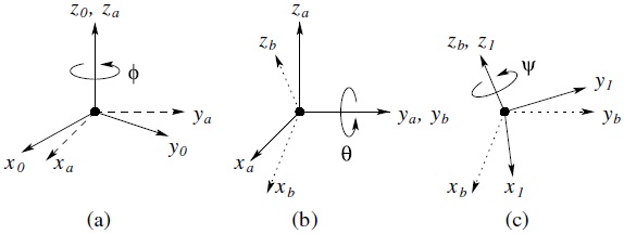
Figure 2.10 Euler angle representation.
In terms of the basic rotation matrices the resulting rotational transformation can be generated as the product

The matrix RZYZ in Equation (2.27) is called the ZYZ–Euler angle transformation.
The more important and more difficult problem is to determine for a particular R = (rij) the set of Euler angles ϕ, θ, and ψ, that satisfy
for a matrix R ∈ SO(3). This problem will be important later when we address the inverse kinematics problem for manipulators in Chapter 5.
To find a solution for this problem we break it down into two cases. First, suppose that not both of r13, r23 are zero. Then from Equation (2.27) we deduce that sθ ≠ 0, and hence that not both of r31, r32 are zero. If not both r13 and r23 are zero, then r33 ≠ ±1, and we have cθ = r33, ![]() so
so
or
where the function Atan2 is the two-argument arctangent function defined in Appendix A.
If we choose the value for θ given by Equation (2.29), then sθ > 0, and
If we choose the value for θ given by Equation (2.30), then sθ < 0, and
Thus, there are two solutions depending on the sign chosen for θ.
If r13 = r23 = 0, then the fact that ![]() is orthogonal implies that r33 = ±1, and that r31 = r32 = 0. Thus,
is orthogonal implies that r33 = ±1, and that r31 = r32 = 0. Thus, ![]() has the form
has the form
If r33 = 1, then cθ = 1 and sθ = 0, so that θ = 0. In this case, Equation (2.27) becomes

Thus, the sum ϕ + ψ can be determined as
Since only the sum ϕ + ψ can be determined in this case, there are infinitely many solutions. In this case, we may take ϕ = 0 by convention. If r33 = −1, then cθ = −1 and sθ = 0, so that θ = π. In this case Equation (2.27) becomes

The solution is thus
As before there are infinitely many solutions.
2.5.2 Roll, Pitch, Yaw Angles
A rotation matrix ![]() can also be described as a product of successive rotations about the principal coordinate axes x0, y0, and z0 taken in a specific order. These rotations define the roll, pitch, and yaw angles, which we shall also denote ϕ, θ, ψ, and which are shown in Figure 2.11.
can also be described as a product of successive rotations about the principal coordinate axes x0, y0, and z0 taken in a specific order. These rotations define the roll, pitch, and yaw angles, which we shall also denote ϕ, θ, ψ, and which are shown in Figure 2.11.
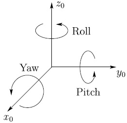
Figure 2.11 Roll, pitch, and yaw angles.
We specify the order of rotation as x − y − z, in other words, first a yaw about x0 through an angle ψ, then pitch about the y0 by an angle θ, and finally roll about the z0 by an angle ϕ.2 Since the successive rotations are relative to the fixed frame, the resulting transformation matrix is given by

Of course, instead of yaw-pitch-roll relative to the fixed frames we could also interpret the above transformation as roll-pitch-yaw, in that order, each taken with respect to the current frame. The end result is the same matrix as in Equation (2.39).
The three angles ϕ, θ, and ψ can be obtained for a given rotation matrix using a method that is similar to that used to derive the Euler angles above.
2.5.3 Axis-Angle Representation
Rotations are not always performed about the principal coordinate axes. We are often interested in a rotation about an arbitrary axis in space. This provides both a convenient way to describe rotations, and an alternative parameterization for rotation matrices. Let k = (kx, ky, kz), expressed in the frame o0x0y0z0, be a unit vector defining an axis. We wish to derive the rotation matrix ![]() representing a rotation of θ about this axis.
representing a rotation of θ about this axis.
There are several ways in which the matrix ![]() can be derived. One approach is to note that the rotational transformation
can be derived. One approach is to note that the rotational transformation ![]() will bring the world z-axis into alignment with the vector k. Therefore, a rotation about the axis k can be computed using a similarity transformation as
will bring the world z-axis into alignment with the vector k. Therefore, a rotation about the axis k can be computed using a similarity transformation as
From Figure 2.12 we see that

Note that the final two equations follow from the fact that k is a unit vector. Substituting Equations (2.42) and (2.43) into Equation (2.41), we obtain after some lengthy calculation (Problem 2–17)
where vθ = vers θ = 1 − cθ.
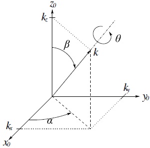
Figure 2.12 Rotation about an arbitrary axis.
In fact, any rotation matrix ![]() can be represented by a single rotation about a suitable axis in space by a suitable angle,
can be represented by a single rotation about a suitable axis in space by a suitable angle,
where k is a unit vector defining the axis of rotation, and θ is the angle of rotation about k. The pair (k, θ) is called the axis-angle representation of ![]() . Given an arbitrary rotation matrix
. Given an arbitrary rotation matrix ![]() with components rij, the equivalent angle θ and equivalent axis k are given by the expressions
with components rij, the equivalent angle θ and equivalent axis k are given by the expressions
and

These equations can be obtained by direct manipulation of the entries of the matrix given in Equation (2.44). The axis-angle representation is not unique since a rotation of − θ about − k is the same as a rotation of θ about k, that is,
If θ = 0 then ![]() is the identity matrix and the axis of rotation is undefined.
is the identity matrix and the axis of rotation is undefined.
Example 2.9.
Suppose ![]() is generated by a rotation of 90° about z0 followed by a rotation of 30° about y0 followed by a rotation of 60° about x0. Then
is generated by a rotation of 90° about z0 followed by a rotation of 30° about y0 followed by a rotation of 60° about x0. Then
We see that ![]() and hence the equivalent angle is given by Equation (2.46) as
and hence the equivalent angle is given by Equation (2.46) as
The equivalent axis is given from Equation (2.46) as
The above axis-angle representation characterizes a given rotation by four quantities, namely the three components of the equivalent axis k and the equivalent angle θ. However, since the equivalent axis k is given as a unit vector only two of its components are independent. The third is constrained by the condition that k is of unit length. Therefore, only three independent quantities are required in this representation of a rotation ![]() . We can represent the equivalent axis-angle by a single vector r as
. We can represent the equivalent axis-angle by a single vector r as
Note, since k is a unit vector, that the length of the vector r is the equivalent angle θ and the direction of r is the equivalent axis k.
One should be careful to note that the representation in Equation (2.51) does not mean that two axis-angle representations may be combined using standard rules of vector algebra, as doing so would imply that rotations commute which, as we have seen, is not true in general.
2.5.4 Exponential Coordinates
In this section we introduce the so-called exponential coordinates and give an alternate description of the axis-angle transformation (2.44). We showed above in Section 2.5.3 that any rotation matrix R ∈ SO(3) can be expressed as an axis-angle matrix Rk, θ using Equation (2.44). The components of the vector ![]() are called exponential coordinates of R.
are called exponential coordinates of R.
To see why this terminology is used, we first recall from Appendix B the definition of so(3) as the set of 3 × 3 skew-symmetric matrices S satisfying
For ![]() let S(k) be the skew-symmetric matrix
let S(k) be the skew-symmetric matrix
and let eS(k)θ be the matrix exponential as defined in Appendix B
Then we have the following proposition, which gives an important relationship between SO(3) and so(3).
Proposition 2.1
The matrix eS(k)θ is an element of SO(3) for any S(k) ∈ so(3) and, conversely, every element of SO(3) can be expressed as the exponential of an element of so(3).
Proof: To show that the matrix eS(k)θ is in SO(3) we need to show that eS(k)θ is an orthogonal matrix with determinant equal to + 1. To show this we rely on the following properties that hold for any n × n matrices A and B

- If the n × n matrices A and B commute, i.e., AB = BA, then eAeB = e(A + B)
- The determinant
 , where tr(A) is the trace of A.
The first two properties above can be shown by direct calculation using the series expansion (2.54) for eA. The third property follows from the Jacobi Identity (Appendix B). Now, since ST = −S, if S is skew-symmetric, then S and ST clearly commute. Therefore, with S = S(kθ) ∈ so(3), we have
which shows that eS(kθ) is an orthogonal matrix. Also
since the trace of a skew-symmetric matrix is zero. Thus eS(kθ) ∈ SO(3) for S(kθ) ∈ so(3).
The converse, namely, that every element of SO(3) is the exponential of an element of so(3), follows from the axis-angle representation of R and Rodrigues’ formula, which we derive next.
Rodrigues’ Formula
Given the skew-symmetric matrix S(k) it is easy to show that S3(k) = −S(k), from which it follows that S4(k) = −S2(k), etc. Thus the series expansion for eS(k)θ reduces to
the latter equality following from the series expansion of the sine and cosine functions. The expression
is known as Rodrigues’ formula. It can be shown by direct calculation that the angle-axis representation for Rk, θ given by Equation (2.44) and Rodrigues’ formula in Equation (2.57) are identical.
Remark 2.1.
The above results show that the matrix exponential function defines a one-to-one mapping from so(3) onto SO(3). Mathematically, so(3) is a Lie algebra and SO(3) is a Lie group.
2.6 Rigid Motions
We have now seen how to represent both positions and orientations. We combine these two concepts in this section to define a rigid motion and, in the next section, we derive an efficient matrix representation for rigid motions using the notion of homogeneous transformation.
Definition 2.2.
A rigid motion is an ordered pair (d, R) where ![]() and R ∈ SO(3). The group of all rigid motions is known as the special Euclidean group and is denoted by SE(3). We see then that
and R ∈ SO(3). The group of all rigid motions is known as the special Euclidean group and is denoted by SE(3). We see then that ![]() .
.
A rigid motion is a pure translation together with a pure rotation.3 Let ![]() be the rotation matrix that specifies the orientation of frame o1x1y1z1 with respect to o0x0y0z0, and
be the rotation matrix that specifies the orientation of frame o1x1y1z1 with respect to o0x0y0z0, and ![]() be the vector from the origin of frame o0x0y0z0 to the origin of frame o1x1y1z1. Suppose the point
be the vector from the origin of frame o0x0y0z0 to the origin of frame o1x1y1z1. Suppose the point ![]() is rigidly attached to coordinate frame o1x1y1z1, with local coordinates
is rigidly attached to coordinate frame o1x1y1z1, with local coordinates ![]() . We can express the coordinates of
. We can express the coordinates of ![]() with respect to frame o0x0y0z0 using
with respect to frame o0x0y0z0 using
Now consider three coordinate frames o0x0y0z0, o1x1y1z1, and o2x2y2z2. Let d1 be the vector from the origin of o0x0y0z0 to the origin of o1x1y1z1 and d2 be the vector from the origin of o1x1y1z1 to the origin of o2x2y2z2. If the point p is attached to frame o2x2y2z2 with local coordinates ![]() , we can compute its coordinates relative to frame o0x0y0z0 using
, we can compute its coordinates relative to frame o0x0y0z0 using
and
The composition of these two equations defines a third rigid motion, which we can describe by substituting the expression for ![]() from Equation (2.59) into Equation (2.60)
from Equation (2.59) into Equation (2.60)
Since the relationship between ![]() and
and ![]() is also a rigid motion, we can equally describe it as
is also a rigid motion, we can equally describe it as
Comparing Equations (2.61) and (2.62) we have the relationships
Equation (2.63) shows that the orientation transformations can simply be multiplied together and Equation (2.64) shows that the vector from the origin o0 to the origin o2 has coordinates given by the sum of ![]() (the vector from o0 to o1 expressed with respect to o0x0y0z0) and
(the vector from o0 to o1 expressed with respect to o0x0y0z0) and ![]() (the vector from o1 to o2, expressed in the orientation of the coordinate frame o0x0y0z0).
(the vector from o1 to o2, expressed in the orientation of the coordinate frame o0x0y0z0).
2.6.1 Homogeneous Transformations
One can easily see that the calculation leading to Equation (2.61) would quickly become intractable if a long sequence of rigid motions were considered. In this section we show how rigid motions can be represented in matrix form so that composition of rigid motions can be reduced to matrix multiplication as was the case for composition of rotations.
In fact, a comparison of Equations (2.63) and (2.64) with the matrix identity
where 0 denotes the row vector (0, 0, 0), shows that the rigid motions can be represented by the set of matrices of the form
Transformation matrices of the form given in Equation (2.66) are called homogeneous transformations. A homogeneous transformation is therefore nothing more than a matrix representation of a rigid motion and we will use SE(3) interchangeably to represent both the set of rigid motions and the set of all 4 × 4 matrices ![]() of the form given in Equation (2.66).
of the form given in Equation (2.66).
Using the fact that ![]() is orthogonal it is an easy exercise to show that the inverse transformation
is orthogonal it is an easy exercise to show that the inverse transformation ![]() is given by
is given by
In order to represent the transformation given in Equation (2.58) by a matrix multiplication, we must augment the vectors ![]() and
and ![]() by the addition of a fourth component of 1 as follows,
by the addition of a fourth component of 1 as follows,
The vectors ![]() and
and ![]() are known as homogeneous representations of the vectors
are known as homogeneous representations of the vectors ![]() and
and ![]() , respectively. It can now be seen directly that the transformation given in Equation (2.58) is equivalent to the (homogeneous) matrix equation
, respectively. It can now be seen directly that the transformation given in Equation (2.58) is equivalent to the (homogeneous) matrix equation
A set of basic homogeneous transformations generating SE(3) is given by
for translation and rotation about the x, y, z-axes, respectively.
The most general homogeneous transformation that we will consider may be written now as
In the above equation n = (nx, ny, nz) is a vector representing the direction of x1 in the o0x0y0z0 frame, s = (sx, sy, sz) represents the direction of y1, and a = (ax, ay, az) represents the direction of z1. The vector d = (dx, dy, dz) represents the vector from the origin o0 to the origin o1 expressed in the frame o0x0y0z0. The rationale behind the choice of letters n, s, and a is explained in Chapter 3.
The same interpretation regarding composition and ordering of transformations holds for 4 × 4 homogeneous transformations as for 3 × 3 rotations. Given a homogeneous transformation H01 relating two frames, if a second rigid motion, represented by H ∈ SE(3) is performed relative to the current frame, then
whereas if the second rigid motion is performed relative to the fixed frame, then
Example 2.10.
The homogeneous transformation matrix ![]() that represents a rotation by angle α about the current x-axis followed by a translation of b units along the current x-axis, followed by a translation of d units along the current z-axis, followed by a rotation by angle θ about the current z-axis, is given by
that represents a rotation by angle α about the current x-axis followed by a translation of b units along the current x-axis, followed by a translation of d units along the current z-axis, followed by a rotation by angle θ about the current z-axis, is given by
2.6.2 Exponential Coordinates for General Rigid Motions
Just as we represented rotation matrices as exponentials of skew-symmetric matrices, we can also represent homogeneous transformations as exponentials using so-called twists.
Definition 2.3.
Let v and k be vectors in ![]() with k a unit vector. A twist ξ defined by k and v is the 4 × 4 matrix
with k a unit vector. A twist ξ defined by k and v is the 4 × 4 matrix
We define se(3) as
se(3) is the vector space of twists, and a similar argument as before in Section 2.5.4 can be used to show that, given any twist ξ ∈ se(3) and angle ![]() , the matrix exponential of ξθ is an element of SE(3) and, conversely, every homogeneous transformation (rigid motion) in SE(3) can be expressed as the exponential of a twist. We omit the details here.
, the matrix exponential of ξθ is an element of SE(3) and, conversely, every homogeneous transformation (rigid motion) in SE(3) can be expressed as the exponential of a twist. We omit the details here.
2.7 Chapter Summary
In this chapter, we have seen how matrices in SE(n) can be used to represent the relative position and orientation of two coordinate frames for n = 2, 3. We have adopted a notional convention in which a superscript is used to indicate a reference frame. Thus, the notation ![]() represents the coordinates of the point p relative to frame 0.
represents the coordinates of the point p relative to frame 0.
The relative orientation of two coordinate frames can be specified by a rotation matrix, R ∈ SO(n), with n = 2, 3. In two dimensions, the orientation of frame 1 with respect to frame 0 is given by
in which θ is the angle between the two coordinate frames. In the three-dimensional case, the rotation matrix is given by

In each case, the columns of the rotation matrix are obtained by projecting an axis of the target frame (in this case, frame 1) onto the coordinate axes of the reference frame (in this case, frame 0).
The set of n × n rotation matrices is known as the special orthogonal group of order n, and is denoted by SO(n). An important property of these matrices is that R− 1 = RT for any R ∈ SO(n).
Rotation matrices can be used to perform coordinate transformations between frames that differ only in orientation. We derived rules for the composition of rotational transformations as
for the case where the second transformation, R, is performed relative to the current frame and
for the case where the second transformation, R, is performed relative to the fixed frame.
In the three-dimensional case, a rotation matrix can be parameterized using three angles. A common convention is to use the Euler angles (ϕ, θ, ψ), which correspond to successive rotations about the z, y, and z-axes. The corresponding rotation matrix is given by
Roll, pitch, and yaw angles are similar, except that the successive rotations are performed with respect to the fixed, world frame instead of being performed with respect to the current frame.
Homogeneous transformations combine rotation and translation. In the three-dimensional case, a homogeneous transformation has the form
The set of all such matrices comprises the set SE(3), and these matrices can be used to perform coordinate transformations, analogous to rotational transformations using rotation matrices.
Homogeneous transformation matrices can be used to perform coordinate transformations between frames that differ in orientation and translation. We derived rules for the composition of rotational transformations as
for the case where the second transformation, H, is performed relative to the current frame and
for the case where the second transformation, H, is performed relative to the fixed frame.
We also defined the vector spaces
and showed that elements of SO(3) and SE(3) can be expressed as matrix exponentials of elements of so(3) and se(3). Formally, SO(3) and SE(3) are Lie groups and so(3) and se(3) are their associated Lie algebras.
Problems
- Using the fact that v1 · v2 = vT1v2, show that the dot product of two free vectors does not depend on the choice of frames in which their coordinates are defined.
- Show that the length of a free vector is not changed by rotation, that is, that ‖v‖ = ‖Rv‖.
- Show that the distance between points is not changed by rotation, that is, ‖p1 − p2‖ = ‖Rp1 − Rp2‖.
- If a matrix R satisfies RTR = I, show that the column vectors of R are of unit length and mutually perpendicular.
-
If a matrix R satisfies RTR = I, then
a) Show that
b) Show that
 if we restrict ourselves to right-handed coordinate frames.
 - Verify Equations (2.4)–(2.6).
- A group is a set X together with an operation * defined on that set such that
- x1*x2 ∈ X for all x1, x2 ∈ X
- (x1*x2)*x3 = x1*(x2*x3)
- There exists an element I ∈ X such that I*x = x*I = x for all x ∈ X
- For every x ∈ X, there exists some element y ∈ X such that x*y = y*x = I
- Derive Equations (2.7) and (2.8).
- Suppose A is a 2 × 2 rotation matrix. In other words ATA = I and
 . Show that there exists a unique θ such that A is of the form

- Consider the following sequence of rotations:
- Rotate by ϕ about the world x-axis.
- Rotate by θ about the current z-axis.
- Rotate by ψ about the world y-axis.
- Consider the following sequence of rotations:
- Rotate by ϕ about the world x-axis.
- Rotate by θ about the world z-axis.
- Rotate by ψ about the current x-axis.
- Consider the following sequence of rotations:
- Rotate by ϕ about the world x-axis.
- Rotate by θ about the current z-axis.
- Rotate by ψ about the current x-axis.
- Rotate by α about the world z-axis.
- Consider the following sequence of rotations:
- Rotate by ϕ about the world x-axis.
- Rotate by θ about the world z-axis.
- Rotate by ψ about the current x-axis.
- Rotate by α about the world z-axis.
-
If the coordinate frame o1x1y1z1 is obtained from the coordinate frame o0x0y0z0 by a rotation of
 about the x-axis followed by a rotation of
  about the fixed y-axis, find the rotation matrix R representing the composite transformation. Sketch the initial and final frames.
 -
Suppose that three coordinate frames o1x1y1z1, o2x2y2z2, and o3x3y3z3 are given, and suppose
Find the matrix
 .
. - Derive equations for the roll, pitch, and yaw angles corresponding to the rotation matrix R = (rij).
- Verify Equation (2.44).
- Verify Equation (2.46).
-
If
 is a rotation matrix show that + 1 is an eigenvalue of
  . Let k be a unit eigenvector corresponding to the eigenvalue + 1. Give a physical interpretation of k.
 -
Let
 , θ = 90°. Find
  .
. -
Show by direct calculation that
 given by Equation (2.44) is equal to
  given by Equation (2.48) if θ and k are given by Equations (2.49) and (2.50), respectively.
 -
Compute the rotation matrix given by the product
-
Suppose
 represents a rotation of 90° about y0 followed by a rotation of 45° about z1. Find the equivalent axis-angle to represent
  . Sketch the initial and final frames and the equivalent axis vector k.
 -
Find the rotation matrix corresponding to the Euler angles
 θ = 0, and
  . What is the direction of the x1 axis relative to the base frame?
 - Unit magnitude complex numbers a + ib with a2 + b2 = 1 can be used to represent orientation in the plane. In particular, for the complex number a + ib, we can define the angle θ = Atan2(a, b). Show that multiplication of two complex numbers corresponds to addition of the corresponding angles.
- Show that complex numbers together with the operation of complex multiplication define a group. What is the identity for the group? What is the inverse for a + ib?
-
Complex numbers can be generalized by defining three independent square roots for − 1 that obey the multiplication rules
Using these, we define a quaternion by Q = q0 + iq1 + jq2 + kq3, which is typically represented by the 4-tuple (q0, q1, q2, q3). A rotation by θ about the unit vector n = (nx, ny, nz) can be represented by the unit quaternion
 . Show that such a quaternion has unit norm, that is, q20 + q21 + q22 + q23 = 1.
 -
Using
 , and the results from Section 2.5.3, determine the rotation matrix R that corresponds to the rotation represented by the quaternion (q0, q1, q2, q3).
 - Determine the quaternion Q that represents the same rotation as given by the rotation matrix R.
-
The quaternion Q = (q0, q1, q2, q3) can be thought of as having a scalar component q0 and a vector component q = (q1, q2, q3). Show that the product of two quaternions, Z = XY is given by
Hint: Perform the multiplication (x0 + ix1 + jx2 + kx3)(y0 + iy1 + jy2 + ky3) and simplify the result.
- Show that QI = (1, 0, 0, 0) is the identity element for unit quaternion multiplication, that is, QQI = QIQ = Q for any unit quaternion Q.
-
The conjugate Q* of the quaternion Q is defined as

Show that Q* is the inverse of Q, that is, Q*Q = QQ* = (1, 0, 0, 0).
- Let v be a vector whose coordinates are given by (vx, vy, vz). If the quaternion Q represents a rotation, show that the new, rotated coordinates of v are given by Q(0, vx, vy, vz)Q*, in which (0, vx, vy, vz) is a quaternion with zero as its real component.
-
Let the point p be rigidly attached to the end effector coordinate frame with local coordinates (x, y, z). If Q specifies the orientation of the end effector frame with respect to the base frame, and T is the vector from the base frame to the origin of the end effector frame, show that the coordinates of p with respect to the base frame are given by
(2.77)
in which (0, x, y, z) is a quaternion with zero as its real component.
- Verify Equation (2.67).
-
Compute the homogeneous transformation representing a translation of 3 units along the x-axis followed by a rotation of
 about the current z-axis followed by a translation of 1 unit along the fixed y-axis. Sketch the frame. What are the coordinates of the origin o1 with respect to the original frame in each case?
 - Consider the diagram of Figure 2.13. Find the homogeneous transformations
 representing the transformations among the three frames shown. Show that
  .
. - Consider the diagram of Figure 2.14. A robot is set up 1 meter from a table. The table top is 1 meter high and 1 meter square. A frame o1x1y1z1 is fixed to the edge of the table as shown. A cube measuring 20 cm on a side is placed in the center of the table with frame o2x2y2z2 established at the center of the cube as shown. A camera is situated directly above the center of the block 2 meters above the table top with frame o3x3y3z3 attached as shown. Find the homogeneous transformations relating each of these frames to the base frame o0x0y0z0. Find the homogeneous transformation relating the frame o2x2y2z2 to the camera frame o3x3y3z3.
- In Problem 2–38, suppose that, after the camera is calibrated, it is rotated 90° about z3. Recompute the above coordinate transformations.
- If the block on the table is rotated 90° about z2 and moved so that its center has coordinates [0, .8, .1]T relative to the frame o1x1y1z1, compute the homogeneous transformation relating the block frame to the camera frame; the block frame to the base frame.
- Consult an astronomy book to learn the basic details of the Earth’s rotation about the sun and about its own axis. Define for the Earth a local coordinate frame whose z-axis is the Earth’s axis of rotation. Define t = 0 to be the exact moment of the summer solstice, and the global reference frame to be coincident with the Earth’s frame at time t = 0. Give an expression R(t) for the rotation matrix that represents the instantaneous orientation of the earth at time t. Determine as a function of time the homogeneous transformation that specifies the Earth’s frame with respect to the global reference frame.
-
In general, multiplication of homogeneous transformation matrices is not commutative. Consider the matrix product

Determine which pairs of the four matrices on the right-hand side commute. Explain why these pairs commute. Find all permutations of these four matrices that yield the same homogeneous transformation matrix,
 .
.

Figure 2.13 Diagram for Problem 2–37.

Figure 2.14 Diagram for Problem 2–38.
Notes and References
Rigid body motions and the groups SO(n) and SE(n) are often addressed in mathematics books on the topic of linear algebra. Standard texts for this material include [9], [30], and [49]. These topics are also often covered in applied mathematics texts for physics and engineering, such as [143], [155], and [182]. In addition to these, a detailed treatment of rigid body motion developed with the aid of exponential coordinates and Lie groups is given in [118].
Notes
- 1 We will use
 ,
,  to denote both coordinate axes and unit vectors along the coordinate axes depending on the context.
 - 2 It should be noted that other conventions exist for naming the roll, pitch, and yaw angles.
- 3 The definition of rigid motion is sometimes broadened to include reflections, which correspond to detR = −1. We will always assume in this text that detR = +1 so that R ∈ SO(3).