Example 4.2. Creating a Customized Table of Descriptive Statistics
Goal
Create a table of descriptive statistics. Obtain the statistics through use of standard SAS procedures, and then write the results in a customized style.
Report
|
Example Features
| Data Set | DEMOG |
| Preparatory Steps | PROC FREQ PROC MEANS with NOPRINT and NWAY options |
| Featured Step | DATA step |
| Featured Step Statements and Options | FILE statement: N= option (example uses N=PS, which is valid when sending output to the LISTING destination) PUT statement with column and formatted output when sending output to the LISTING destination |
| Formatting Features | FILE statement: HEADER= and NOTITLES options when sending output to the LISTING destination |
| Creating a Format for Percentages with the PICTURE Statement in PROC FORMAT
Computing Descriptive Statistics Concatenating SAS Data Sets Positioning the Output Line Pointer to a Specific Column by Calculating the Column Position Positioning the Output Line Pointer to a Specific Row by Calculating the Row Position Supplying Heading Information for All Pages | |
| ODS Enhanced Version of This Example | Example 6.12 |
| Other Examples That Use This Data Set | Example 6.12 |
Example Overview
This report compares the demographic data of subjects assigned to two treatment groups in a clinical trial. It mixes frequencies and statistics within the content of the report. The required structure of the table cannot be achieved with PROC TABULATE or PROC REPORT.
The FREQ and MEANS procedures summarize the data and output the results to data sets. There are six sections in the report, and the program creates an output data set from either PROC FREQ or PROC MEANS for each section. A DATA step concatenates these data sets, uses conditional processing to write rows in the report, and produces the report’s headings.
Each observation in the DEMOG data set corresponds to all the measurements on one patient in one treatment group.
The sole destination of this example is intended to be the LISTING destination. The PUT statements in the DATA step write output to specific row and column positions. The same output sent to a nonlisting destination would not look properly formatted. Example 6.12 uses ODS features to construct a similar report that is sent to a nonlisting destination.
This example works with data sets produced by PROC FREQ and PROC MEANS. You can also save your output in data sets produced by ODS output objects. Example 4.3 creates a customized report from data sets produced by ODS output objects.
Program
|
| A Closer Look |
Creating a Format for Percentages with the PICTURE Statement in PROC FORMAT
The PERCEN. format writes percentage values according to the templates, or pictures, in the PICTURE statement. The ROUND option rounds off values to the closest integer. If a value ends in 0.5, it is rounded up.
picture percen (round) .=' ( %)' (noedit)
other ='0009%)'
(prefix ='('),The first picture, which is for missing values, writes parentheses with a percent sign, but no number. The NOEDIT option means that the PICTURE format writes the characters between quotes exactly as they appear in the statement for the specified value or values.
For the picture for all nonmissing values, the string “0009” specifies placeholders for the formatted value. The PREFIX= option writes the open parenthesis before the first digit. The prefix character counts as one of the positions in the picture. The remaining three positions in the picture, represented by the second and the third 0 and the 9, are reserved for the percentage value. The placeholder of 0 specifies that no leading zero is written in that position. That is, if the value that is being formatted is less than 10, the left parenthesis will be put in the position of the third 0 in the picture.
Computing Descriptive Statistics
PROC MEANS provides data summarization tools that compute descriptive statistics for variables across all observations and within groups of observations. The program in this example executes three simple PROC MEANS steps. Each execution computes a few statistics on one analysis variable for groups defined by the values of one classification variable. The results are saved in output data sets.
The OUTPUT statement tells SAS to save specific statistics in an output data set. Specify each keyword for a statistic that you want to save and follow the keyword with an equal sign and the variable name that you want to assign to the statistic in the output data set. In this example, the variable names are the same as the keyword names.
The class variable TMTDG has two values, and each of the three output data sets produced by the three PROC MEANS steps has two observations, one for each value of TMTDG. The first observation in each output data set contains the statistics for the active group and the second observation contains the statistics for the placebo group.
PROC MEANS supports many variations on the form of the OUTPUT statement for computing statistics, providing variable names, and identifying specific observations. Saving these seven statistics is just a small sampling of what you can do with the OUTPUT statement in PROC MEANS. See Example 3.2 for more detail on using PROC MEANS.
Concatenating SAS Data Sets
The SET statement reads one observation on each iteration of the DATA step. It reads all the observations from the first data set, then the second, and so on, until it has read all observations from all six data sets:
set t1(in=in1) t2(in=in2) t3(in=in3) t4(in=in4)
t5(in=in5) t6(in=in6);The IN= data set option creates a variable that indicates whether the data set contributed to the current observation (1=true and 0=false). The values of the variables IN1 through IN6 are used in conditional processing to write different rows in the report.
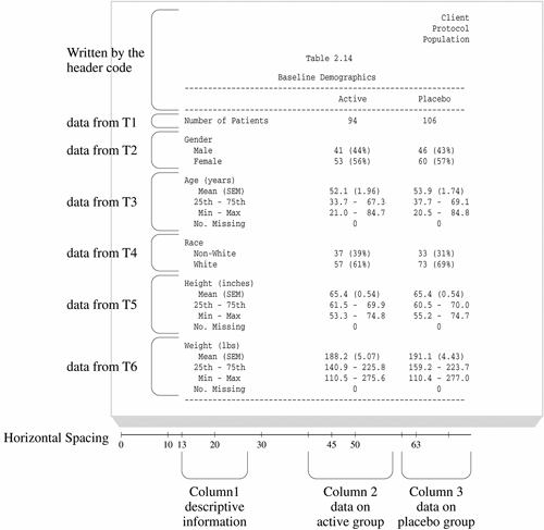
Figure 4.2 identifies rows and columns in the report and shows which of the six data sets contributes to each row. Note the similar structure of the data on gender and race from data sets T2 and T4 and the similar structure of the data on age, height, and weight from data sets T3, T5, and T6. Because these sections of the report are so similar, the same code can be used to produce the rows describing GENDER and RACE, and the same code can be used to produce the rows on AGE, HEIGHT, and WEIGHT.
Positioning the Output Line Pointer to a Specific Column by Calculating the Column Position
This program is written to send output to the LISTING destination. Therefore, it can direct output to specific columns on the report page.
This program uses the variable COL to position the pointer when centering text under “Active” and “Placebo” in the report. The value of COL is derived by applying the informat COLPLC to the variable TMTDG.
proc format;
  invalue colplc 'Active'=45
                 'Placebo'=63;
The INPUT function reads the value of TMTDG, applies the informat COLPLC to the values of TMTDG, returns the value 45 or 63, and assigns one of these numeric values to COL.
col=input(tmtdg,colplc.);
All data written in the “Active” column is centered on column 45, and data in the “Placebo” column is centered on column 63. Many PUT statements in this program use the value of COL to correctly position text in these columns. Here are some examples:
| □ | put...@(col-1) count pct_row percen5.; |
| □ | put...@(col-2) mean 4.1 |
| □ | put...@(col+3) '(' stderr 4.2 ')' |
Using this indirect method to determine where to place a value has two advantages:
| □ | It puts the literal value in one location so that if you need to move that column in the report, you can make one change and yet keep the data aligned. |
| □ | It uses one variable value for two purposes: to place the data in the correct treatment column (“Active” or “Placebo”) and to center the data under the column headings. |
Positioning the Output Line Pointer to a Specific Row by Calculating the Row Position
The following lines of code write the rows on gender data when reading from data set T2 (IN2 is true) and the rows on race data when reading from T4. (Because this code is part of a larger DO group that reads only from data sets T2 or T4, the ELSE block processes data only from T4.)
if in2 then put 2 #(row+gender) @15 gender gendrfmt.
               1 @(col-1) count pct_row percen5.;
else put 2 #(row+race) @15 race racefmt.
        1 @(col-1) count pct_row percen5.;
if inds=4 then inds=0; 3
|
| The use of the variable COL to position the pointer based on the value “Active” (45) or “Placebo” (63) is discussed in the previous section. |
|
| Similar to the way COL is used in conjunction with the current values of TMTDG, the values of ROW, GENDER, and RACE are used to position the pointer on the correct row based on the current value of GENDER or RACE. For example, when the observation contains data on “Male,” the true value of GENDER is 0, so those values are written on the row equal to the current value of the variable ROW. When the observation contains data on “Female,” the true value of GENDER is 1, so those values are written one row after the row for “Male.” |
|
| There are only four observations in each of the two data sets. When INDS equals 4, the DATA step reads the last observation in the data set currently being processed. It resets INDS to zero because the next observation that the DATA step processes will be from a new data set. |
Supplying Heading Information for All Pages
To print headings at the top of each new page of a report:
| □ | specify a label with the HEADER= option in a FILE statement |
| □ | place a RETURN statement before the statement label |
| □ | place a colon after the label |
| □ | place the statements that construct the heading after the statement label |
| □ | place a RETURN statement at the end of these statements. |
Here is the code that creates the heading for this report, followed by an explanation:
file 'external-file' print n=ps notitles header=reporttop; 1

return; 2

reporttop: 3
  put #2  @67 'Client' 4
      #3  @65 'Protocol'
      #4  @63 'Population'
      #6  @38 'Table  2.14'
      #8  @32 'Baseline Demographics'
      #9  @13 60*'-'
      #10 @45 'Active' @62 'Placebo'
      #11 @13 60*'-';
  row=12; 5
  return; 6
run;
|
| The FILE statement specifies REPORTTOP as the statement label. |
|
| The RETURN statement that precedes the label is necessary to prevent the statements following the label from executing with each iteration of the DATA step. |
|
| The statement label is followed by a colon. |
|
| The PUT statement produces the heading on this single-page report by writing data on eight lines. |
|
| The assignment statement assigns a value of 12 to ROW after the heading is written. That value is used to position the next line of text in the report, which corresponds to the first line of the results. |
|
| The RETURN statement signals the end of the section labeled REPORTTOP. |
Where to Go from Here
Concatenating data sets. See “Combining SAS Data Sets: Basic Concepts” and “Combining SAS Data Sets: Methods” in the “Reading, Combining, and Modifying SAS Data Sets” section of SAS 9.1 Language Reference: Concepts, and “SET Statement” in the “Statements” section of SAS 9.1 Language Reference: Dictionary.
Description of how SAS processes a DATA step. See “DATA Step Processing” in the “Data Step Concepts” section of SAS 9.1 Language Reference: Concepts.
FILE statement syntax, usage information, and additional examples. See “FILE Statement” in the “Statements” section of SAS 9.1 Language Reference: Dictionary.
The IN= data set option used on the SET statement. See “SET Statement” in the “Statements” section of SAS 9.1 Language Reference: Dictionary.
INPUT function syntax, usage informaton, and additional examples. See “INPUT Function” in the “Functions and CALL Routines” section of SAS 9.1 Language Reference: Concepts.
More Examples of Writing a Report with a DATA Step. See “Writing a Report with a DATA Step” in the “DATA Step Processing” section of SAS 9.1 Language Reference: Concepts.
PROC FORMAT reference, usage information, and additional examples. See “The FORMAT Procedure” in Base SAS 9.1 Procedures Guide.
PROC FREQ reference, usage information, and additional examples. See “The FREQ Procedure” in Base SAS 9.1 Procedures Guide.
PROC MEANS reference, usage information, and additional examples. See “The MEANS Procedure” in Base SAS 9.1 Procedures Guide.
PUT statement syntax, usage information, and additional examples. See “PUT Statement,” “PUT Statement, Column,” “PUT Statement, Formatted,” and “PUT Statement, List” in the “Statements” section of SAS 9.1 Language Reference: Dictionary.
SET statement syntax, usage information, and additional examples. See “SET Statement” in the “Statements” section of SAS 9.1 Language Reference: Dictionary.
Working with Formats. See “Formats and Informats” in “SAS Language Elements” in the “SAS System Concepts” section of SAS 9.1 Language Reference: Concepts, and “Formats” in Base SAS 9.1 Language Reference: Dictionary.