Chapter 2: Using the Designer

SAS Release	Start the Designer
9.2 Phase 2	Submit the following macro from the SAS program window: %sgdesign();
9.3 and 9.4	Submit the previous macro or select Tools ► ODS Graphics Designer.

The designer opens in a separate window.

To access SAS data sets and other SAS functionality, the designer works in conjunction with another open SAS session. The designer does not work in the SAS session from which it was launched. To accomplish this, when the designer is launched, it opens a new, in-the-background SAS session on the same computer and works in that SAS session to create the graphs.

To create graphs from your data, the designer needs to know the libraries that you have been working with before launching. Therefore, relevant information about all active libraries is sent to the designer, and active libraries are assigned (in a new SAS session) to access your data sets. For more information, see “Parameters Available for the SGDESIGN Macro” at the end of this chapter.

Designer Graphical User Interface

When the designer starts, it displays a graphical user interface in a separate window.

Tip: Sometimes this window might be hidden behind the SAS application window. If so, click on the designer icon () in the taskbar to bring it to the front.

Here are the features of the designer’s main window:

Figure 2.1 The Designer’s Main Window

1. The main menu bar contains menus that you can use to perform a variety of tasks within the designer.

2. The Elements pane contains plots, lines, and insets that you can insert into a graph. To insert an element, click and drag the element onto the graph. The elements in this pane are available only when a graph is open.

3. The toolbar contains icons that you can click to perform common tasks such as saving files and inserting titles or footnotes. The icons on this toolbar are available only when a graph is open.

4. The work area contains one or more graphs that you create and design in the designer. In addition to the graphs, you can display the Graph Gallery, a collection of predefined graphs.

Menus and Toolbar

The main menu bar provides options for managing graphs, graphics elements, and other features. Common menu options are also available on the toolbar.

Here are the menus and their tasks:

File

open, save, and print graphs. You can save graphs in several formats, and you can save a graph to the Graph Gallery.

You can export styles that you have created or modified. Creating and editing styles is beyond the scope of this book.

Edit

undo and redo your actions. You can copy a graph image to the clipboard and then immediately paste it into another application.

View

display or hide the Graph Gallery and the Elements pane.

The designer generates GTL code behind the scenes to create the graphs that are being built. You can show or hide the code window from this menu.

Insert

insert graphics elements such as titles, footnotes, and global legends into a graph.

Format

modify visual properties of the selected plot. You can apply a different style to the graph.

Tools

open the style editor tool. You can also update user preferences.

Help

view the designer’s About dialog box. Starting with the third maintenance release for SAS 9.4, the menu contains a link to online Help.

Graph Gallery

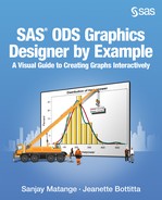
The work area is on the right side of the main window. It contains the Graph Gallery as shown in Figure 2.2. This gallery provides predefined, commonly used graphs that you can create. The Graph Gallery is organized into groups of graphs. Each group is represented as a tab in the gallery. The following figure shows the default view of the graph icons that are on the Basic tab.

Click on the various tabs to explore the graphs.

Figure 2.2 Graph Gallery

You can choose a predefined graph as the basis for your graph. You can then customize your graph by adding titles, footnotes, legends, additional plots, and other items.

In addition to the predefined graphs, you can add your own custom graphs to the Graph Gallery.

Elements Pane: Plots and Insets

The Elements pane is to the left of the work area. This pane contains icons for the plots and insets that you can add to a graph.

Figure 2.3 Elements Pane

The elements in this pane are available only when a graph is open.

The Elements pane contains the following panels:

● The Plot Layers panel contains icons for different plot types that can be used to design many types of graphs. All of the elements in this panel are plots and lines.

● The Insets panel contains icons for graphics elements including a discrete legend, a gradient legend (for contour plots), a cell header, and a text entry.

Right-Click Pop-Up Menus

Pop-up menus are available for most aspects of a graph. These handy menus apply to plots, legends, axes, graph cells, titles, footnotes, and the graph itself. For example, if you right-click inside a graph cell, and select Add an Element, a dialog box is displayed from which you can add a plot, inset, title, footnote, or legend.

Create a Graph

You can create a graph in one of the following ways:

● Select a graph from the Graph Gallery, and click OK. This is perhaps the easiest way to create a graph.

When you open a graph from the gallery, an Assign Data dialog box is displayed, showing the placeholder settings for the plot variables. Change the settings as needed for your graph, and click OK to create the graph. This is discussed in more detail in subsequent chapters.

Tip: If the Graph Gallery is not displayed, select View ► Graph Gallery to display it.

● Select File ► New ► Blank Graph. When you start from a blank graph, you must add all the plots, titles, legends, and other elements to create your graph.

● Open a previously saved graph by selecting File ► Open.

● Use the Auto Charts feature to generate graphs based on your data and the graph types that you specify. This is discussed in Chapter 6.

Once a new graph is created, it is displayed in a graph window in the work area. If there is a graph in the work area, the Elements pane is active. You can then drag and drop compatible plots or insets onto the graph and customize the graph with titles, footnotes, and other graphics elements.

Graph Terminology

Let’s review the terminology used to reference different parts of the graph.

Figure 2.4 Graph Example for Terminology

Term	Description
Graph	The entire entity shown in the example graph.
Cell	A data area of a graph that can contain plots, text, and a legend. The example graph contains two cells.
Plot	A graphical representation of data. In the example graph, the left cell contains a grouped scatter plot and the right cell contains a box plot.
Axis	The axis line, the major and minor tick marks, the major tick mark values, and the axis label. Each cell can have its own independent axes, or the cells can share a common axis. In the example graph, the two cells share the Y axis, but they have their own independent X axes.
Titles and Footnotes	Descriptive text that is displayed above (title) or below (footnote) any cell or plot area in the graph. A graph can have zero or more titles, footnotes, or both. The example graph contains one title, “Vehicle Mileage Data.”
Legend	A legend border and one or more legend entries. A graph can have one or more legends. The legend can reside inside a cell (cell legend) or outside a cell (global legend). In the example graph, the scatter plot includes a cell legend.
Inset	An element displaying relevant information. In the example graph, the right cell contains a text entry inset in the upper right corner of the cell.

Basic Concepts and Task Workflow

Creating graphs involves a simple building-block process. The following list summarizes the main steps that you perform to create a graph. Although the steps are listed in a logical order, the order in which you perform them can vary.

● Start the graph. You can start with a graph from the Graph Gallery, and then add more plots, legends, insets, titles, and so on, to create the custom graph that you need. Or, you can start with a blank graph, add plots, and so on.

Note: The Auto Charts feature enables you to generate a graph based on your data and the graph type that you specify. This is discussed in Chapter 6.

● Add plots, legends, or insets to a graph. If you started with a blank graph, you must add at least one plot.

Drag and drop an item from the Elements pane onto a cell of the graph. You can drag and drop more than one plot onto a cell if the plots are compatible. For example, you might drag and drop a fit plot onto a cell that has a scatter plot with numeric variables. Both are compatible plots.

Often, compatibility can be determined only after the roles and axis settings have been assigned. You might drag and drop a plot that has role assignments that make it incompatible with the current contents of the cell. In this case, a message is displayed, and the new plot is not added.

For more information about plot compatibility, see Chapter 4.

Some non-plot items, such as the discrete legend and text entry inset, are included in the Insets panel of the Elements pane. These items can be dragged and dropped onto a cell.

● Assign data roles to a plot. You assign data roles to a new plot when the plot is added to your graph. Assigned data roles can be changed later using the plot’s right-click pop-up menu.

● Add titles, footnotes, or global legends. These can be inserted into the graph by selecting the Insert menu.

● Assign visual properties to graphs. Visual properties can be assigned by using the plot’s right-click pop-up menu. Similarly, visual properties for axes, legends, titles, and so on, can be assigned by using the appropriate pop-up menu.

● You can save the results as an image file for inclusion in a report or as an ODS Graphics Designer file (SGD) that you can later edit. You can save your graphs in the following formats: HTML, PDF, EMF, and PS.

Graph Types and Layouts

With the designer, you can create the following types and layouts of graphs:

Type and Layout	Example Figure
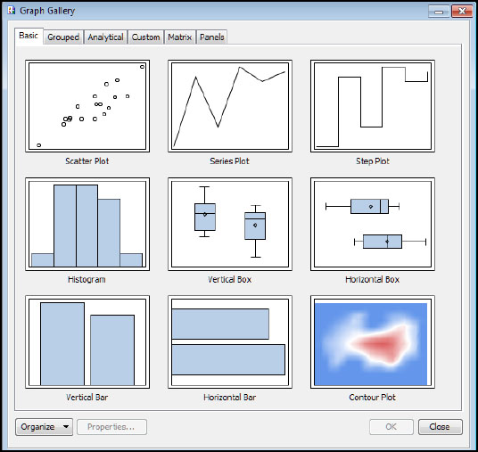
Single-cell graph. This graph has only one cell containing all the plots. The graph can have multiple titles, footnotes, and legends. The data for all the plots in a cell must come from a single data set.
Multi-cell ad hoc graph. This graph has multiple cells that contain plots displaying data. Each cell can have a different set of overlaid plots with legends and insets. This graph can have multiple titles at the top of the graph above all the cells and multiple footnotes at the bottom below all the cells. Each cell can have a different associated data set.
Multi-cell classification panel. This graph has multiple cells arranged in a regular grid. The number and arrangement of the cells are determined by the panel variables. The plot type in each cell is the same, using a subset of data for the crossing of panel variables. Cells cannot have legends or insets. This graph can have multiple titles at the top of the graph above all the cells, and multiple footnotes at the bottom below all the cells. The data for all the plots must come from a single data set.

In addition to these types and layouts, the designer includes shared-variable graphs. In these graphs, different plots are driven by shared variables. Shared-variable graphs support all three layouts described in the previous table. These graphs are discussed in more detail in Chapter 7.

Parameters Available for the SGDESIGN Macro

The SGDESIGN macro that is used to start the designer accepts the following optional parameters:

refresh = Y | N

Default = N. Refresh the list of libraries available to the designer.

While using the designer, you can go into the other open SAS session and continue working with your data sets in the previously assigned libraries, including Work. These new or modified data sets are visible in the designer SAS session. If you modify an existing library assignment or create a new library assignment, you must send that information to the designer before the library can become available. To do this, you can resubmit the SGDESIGN macro with the REFRESH option. This sends the updated information to the designer. Here is an example:

%sgdesign(refresh=y);

portNum = integer

Default = 5310. This parameter indicates the port that the designer uses to communicate with the SAS server. If another application is using port 5310, you can specify a different port for the designer, such as 5320.

dataSets = Y | N

Default = N. This parameter rebuilds the Work data sets. Some of the plots that are provided with the designer depend on data sets that the designer creates in the Work library. If you inadvertently delete some of these data sets, you can re-create them by setting this parameter to Y the next time you start the designer.

For example, to change the port number to 5320 and re-create the data sets, you can submit the following statement:

%sgdesign(portnum=5320, datasets=Y);

These parameters can be used in any order.

..................Content has been hidden....................

You can't read the all page of ebook, please click here login for view all page.

Table of Contents for Chapter 2: Using the Designer

Create new playlist

Sign In

Sign Up