10. Views, Temporary Tables, CTEs, and Indexes
A database is made up of more than just a schema and permanent base tables. It can contain views, temporary tables, and common table expressions (CTEs). It may also contain indexes, which although no longer part of the SQL standard, are supported by most DBMSs for enforcing primary key constraints and speeding retrieval performance.
Views
A view is a virtual table that is produced by executing a SQL-query. It is stored in the data dictionary as a named SELECT. Whenever a SQL query contains the name of a view, the DBMS executes the query associated with the view's definition to create its virtual result table. That table can the be used as a source table by the remainder of the query in which its name appears.
Why Use Views?
There are several important reasons for using views in a database environment:
◊ Views provide a way to store commonly used complex queries in the database. Users can use a simple query such as
SELECT column1, column2, column3
FROM view_name
instead of typing a complex SQL statement.
◊ Views can help maintain database security. Rather than giving users access to entire base tables, you can create views that provide users with exactly the data they need to see. You then grant users access to the views but not to the base tables. (A complete discussion of granting and revoking access rights can be found later in this chapter.)
Creating Views
To create a view whose columns have the same name as the columns in the base table(s) from which it is derived, you give the view and name and include the SQL query that defines its contents:
CREATE VIEW view_name AS
SELECT …
For example, if someone at the rare book store wanted to create a view that would contain data about only leather bound books, the SQL is written
CREATE VIEW leather_bound AS
SELECT author, title
FROM author JOIN work JOIN book
JOIN volume
WHERE UPPER (binding) = ‘LEATHER’;
If you want to rename the columns in the view, you include the new column names in the CREATE VIEW statement:
CREATE VIEW leather_bound (leather_author, leather_title) AS
SELECT author, title
FROM author JOIN work JOIN book
JOIN volume
WHERE UPPER (binding) = ‘LEATHER’;
The preceding statement will produce a view with two columns named leather_author and leather_title. Notice if you want to change even one column name, you must include all column names in the parentheses following the name of the view. The DBMS will match the columns following SELECT with the view column names by their position in the list.
Views can be created from nearly any SQL query, including those that perform joins, unions, and grouping. For example, to simplify looking at sales figures, someone at the rare book store might create a view like the following:
CREATE VIEW sales_summary AS
SELECT customer_numb,
SUM (sale_total_amt)
AS total_purchases
FROM sale
GROUP BY customer_numb;
The view table will then contain grouped data along with a computed column. The beauty of this view is that each time its name is used, the sum will be computed again, ensuring that the data remain up to date.
Note: Views cannot be created from queries that include local tem- porary tables.
Querying Views
You use a view in a SQL SELECT just as you would a base table. For example, to see the entire contents of the sales_summary view created in the preceding section, someone at the rare book store could use the simple query
SELECT *
FROM sales_summary;
which produces the result table in Figure 10-1.
 |
| Figure 10-1 The output of querying a view that includes grouping and a calculated column |
You can apply additional predicates to a view, as in the following example that restricts rows by date:
SELECT *
FROM sales_summary
WHERE total_purchases >= 500;
This time, the result contains only two rows:
| customer_numb | total_purchases |
|---|---|
| 1 | 793.00 |
| 12 | 505.00 |
View Updatability Issues
Theoretically, you should be able to perform INSERT, UPDATE, and DELETE on views as well as SELECT. However, not all views are updatable (capable of being used for updating). Keep in mind that a view's table exists only in main memory. If it is to be used for updates, then the DBMS must be able to propagate the update back to the view's base table(s).
The SQL:2006 places the following restrictions on updatability:
◊ The view must not use UNION DISTINCT, EXCEPT ALL, EXCEPT DISTINCT, or INTERSECT.
◊ Each updatable column in the view must correspond to an updatable column in a source table; each non-up-datable column in the view must correspond to a non-updatable column in a source table.
If you have created a view based on another view, then the underlying view must also be updatable. In addition, you will be unable to insert rows into views that do not contain the primary key columns of their base tables. (Doing so will violate the base table's primary key constraint.) Although updates and deletes are possible when the primary key columns aren't present in a view, performing such modifications may have unexpected results because you can't be certain which rows will be affected. 1
1Some current DBMSs support an INSTEAD OF trigger that lets you create a procedure that updates the underlying table(s) of a view when the view itself isn't updatable. For example, such a procedure might generate values where needed to complete a primary key. However, INSTEAD OF triggers are not part of the SQL standard,
Temporary Tables
A temporary table is a base table that is not stored in the database, but instead exists only while the database session in which it was created is active. At first glance, this may sound like a view, but views and temporary tables are rather different:
◊ A view exists only for a single query. Each time you use the name of a view, its table is recreated from existing data.
◊ A temporary table exists for the entire database session in which it was created.
◊ You must add data to a temporary table with SQL INSERT commands.
◊ Only views that meet the criteria for view updatability can be used for data modification. When you use a view for updating, the updates are permanently propagated to the underlying base tables.
◊ Because temporary tables are base tables, all of them can be updated. However, the updates are as temporary as the table.
◊ Because the contents of a view are generated each time the view's name is used, a view's data are almost always current.
◊ The data in a temporary table reflect the state of the database at the time the table was loaded with data. If the data in table(s) from which the temporary table was loaded are modified after the temporary table has received its data, then the contents of the temporary table may be out of sync with other parts of the database.
If the contents of a temporary table become outdated when source data change, why use a temporary table at all? Wouldn't it be better simply to use a view whose contents are continually regenerated? The answer lies in performance. It takes processing time to create a view table. If you are going to use the data only once during a database session, then a view will actually perform better than a temporary table because you don't need to create a structure for it. However, if you are going to be using the data repeatedly during a session, then a temporary table provides better performance because it needs to be created only once. The decision therefore results in a trade-off. Using a view repeatedly takes more time but provides continually updated data; using a temporary table repeatedly saves time, but you run the risk that the table's contents may be out of date.
Creating Temporary Tables
Creating a temporary table is very similar to creating a permanent base table. You do, however, need to decide on the scope of the table. A temporary table can be global, in which case it is accessible to the entire application program that created it. Alternatively, it can be local, in which case it is accessible only to the program module in which it was created.
To create a global temporary table, you add the keyword GLOBAL TEMPORARY to the CREATE TABLE statement:
CREATE GLOBAL TEMPORARY TABLE
(remainder of CREATE statement)
For example, if someone at the rare book store was going to use the sales summary information repeatedly, then he or she might create the following temporary table instead of using a view:
CREATE GLOBAL TEMPORARY TABLE sales_summary
(customer_numb INT,
total_purchases NUMERIC (7,2),
PRIMARY KEY (customer_numb));
To create a local temporary table, you replace GLOBAL with LOCAL:
CREATE LOCAL TEMPORARY TABLE sales_summary
(customer_numb INT,
total_purchases NUMERIC (7,2),
PRIMARY KEY (customer_numb));
Loading Temporary Tables with Data
To place data in a temporary table, you use one or more SQL INSERT statements. For example, to load the sales_summary table created in the preceding section, you could use
You can now query and manipulate the sales_summary table just as you would a permanent base table.
Disposition of Temporary Table Rows
When you write embedded SQL you have control over the amount of work that the DBMS considers to be a unit (a transaction). We will discuss transactions in depth in Chapter 13. However, to understand what happens to the rows in a temporary table, you do need to know that a transaction can end in one of two ways: It can be committed (its changes made permanent) or it can be rolled back (its changes undone).
By default, the rows in a temporary table are purged whenever a transaction is committed. You can, however, instruct the DBMS to retain the rows by including ON COMMIT PRESERVE ROWS to the end of the table creation statement:
INSERT INTO sales_summary
SELECT customer_numb,
sum (total_sale_amt)
FROM sale
GROUP BY customer numb
ON COMMIT PRESERVE ROWS;
Because a rollback returns the database to the state it was in before the transaction began, a temporary table will also be restored to its previous state (with or without rows).
Common Table Expressions (CTEs)
A common table expression (CTE) is yet another way of extracting a subset of a database for use in another query. CTEs are like views in that they generate virtual tables. However, the definitions of a CTE is not stored in the database and it must be used immediately after it is defined.
To get started, let's look at a very simple example. The general format of a simple CTE is
WITH CTE_name (columns) AS
(SELECT_statement_defining_table)
CTE_query
For example, a CTE and its query to view all of the rare book store's customers could be written
WITH customer_names (first, last) AS
(SELECT first_name, last_name
FROM customer)
SELECT *
FROM customer_names;
The result is a listing of the first and last names of the customers. This type of structure for a simple query really doesn't buy you much except that the CTE isn't stored in the database like a view and doesn't require INSERT statements to populate it like a temporary table. However, the major use of CTEs is for recursive queries, queries that query themselves. (That may sound a bit circular, and it is, intentionally.) The typical application of a recursive query using a CTE is to process hierarchical data, data arranged in a tree structure. It will allow a single query to access every element in the tree or to access subtrees that begin somewhere other than the top of the tree.
As an example, let's create a table that handles the descendants of a single person (in this case, John). As you can see in Figure 10-2, each node in the tree has at most one parent and any number of children. The numbers in the illustration represent the ID of each person.
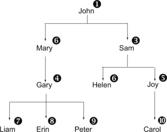 |
| Figure 10-2 A tree structure that can be represented in a relational database and traversed with a recursive query |
Relational databases are notoriously bad at handling this type of hierarchically structured data. The typical way to handle it is to create a relation something like this:
genealogy (person_id, parent_id, person_name)
Each row in the table represents one node in the tree. For this example, the table is populated with the 10 rows in Figure 10-3. John, the node at the top of the tree, has no parent ID. The parent_ID column in the other rows is filled with the person ID of the node above in the tree. (The order of the rows in the table is irrelevant.)
 |
| Figure 10-3 Sample data for use with a recursive query |
We can access every node in the tree by simply accessing every row in the table. However, what can we do if we want to process just the people who are Sam's descendants? There is no easy way with a typical SELECT to do that. However, a CTE used recursively will identify just the rows we want.
The syntax of a recursive query is similar to the simple CTE query with addition of the keyword RECURSIVE following WITH. For our particular example, the query will be written:
WITH RECURSIVE show_tree AS
(SELECT
FROM genealogy
WHERE person_name = ‘Sam’
UNION ALL
SELECT g.*
FROM genealogy as g, show_tree as st
WHERE g.parent_id = st.person_id)
SELECT *
FROM show_tree
ORDER BY person_name;
The result is
| person_id | parent_id | person_name |
|---|---|---|
| 10 | 5 | Carol |
| 6 | 3 | Helen |
| 5 | 3 | Joy |
| 3 | 1 | Sam |
The query that defines the CTE called show_tree has two parts. The first is a simple SELECT that retrieves Sam's row and places it in the result table and in an intermediate table that represents the current state of show_tree. The second SELECT (below UNION ALL) is the recursive part. It will use the intermediate table in place of show_tree each time it executes and add the results of each iteration to the result table. The recursive portion will execute repeatedly until it returns no rows.
Here's how the recursion will work in our example:
1. Join the intermediate result table to genealogy. Because the intermediate result table contains just Sam's row, the join will match Helen and Joy.
2. Remove Sam from the intermediate table and insert Helen and Joy.
3. Append Helen and Joy to the result table.
4. Join the intermediate table to genealogy. The only match from the join will be Carol. (Helen has no children and Joy has only one.)
5. Remove Helen and Joy from the intermediate table and insert Carol.
6. Append Carol to the result table.
7. Join the intermediate table to genealogy. The result will be no rows and the recursion stops.
CTEs cannot be reused; the declaration of the CTE isn't saved. Therefore they don't buy you much for most queries. However, they are enormously useful if you are working with treestructured data. CTEs and recursion can also be helpful when working with bill of materials data.
Indexes
An index is a data structure that provides a fast access path to rows in a table based on the values in one or more columns (the index key). Because the DBMS can use a fast search technique to find the values rather than being forced to search each row in an unordered table sequentially, data retrieval is often much faster.
The conceptual operation of an index is diagrammed in Figure 10-4. (The different weights of the lines have no significance other than to make it easier for you to follow the crossed lines.) In this illustration, you are looking at the work relation and an index that provides fast access to the rows in the table based on a book's title.
 |
| Figure 10-4 The operation of an index to a relation |
The index itself contains an ordered list of keys (the book titles) along with the locations of the associated rows in the book table. The rows in the book table are in relatively random order. However, because the index is in alphabetical order by title, it can be searched quickly to locate a specific title. Then the DBMS can use the information in the index to go directly to the correct row or rows in the book table, thus avoiding a slow sequential scan of the base table's rows.
Once you have created an index, the DBMS's query optimizer will use the index whenever it determines that using the index will speed up data retrieval. You never need to access the index again yourself unless you want to delete it.
When you create a primary key for a table, the DBMS either automatically creates an index for that table using the primary key column or columns as the index key or requires you to create a unique index for the primary key. The first step in inserting a new row into a table is therefore verification that the index key (the primary key of the table) is unique to the index. In fact, uniqueness is enforced by requiring the index entries to be unique, rather than by actually searching the base table. This is much faster than attempting to verify uniqueness directly on the base table because the ordered index can be searched much more rapidly than the unordered base tab
Deciding Which Indexes to Create
You have no choice as to whether the DBMS creates indexes for your primary keys; you get them whether you want them or not. In addition, you can create indexes to provide fast access to any column or combination of columns you want. However, before you jump head first into creating indexes on every column in every table, there are some trade-offs to consider:
◊ Indexes take up space in the database. Given that disk space is relatively inexpensive today, this is usually not a major drawback.
◊ When you insert, modify, or delete data in indexed columns, the DBMS must update the index as well as the base table. This may slow down data modification operations, especially if the tables have a lot of rows.
◊ Indexes definitely speed up access to data.
The trade-off therefore is generally between update speed and retrieval speed. A good rule of thumb is to create indexes for foreign keys and for other columns that are used frequently in WHERE clause predicates. If you find that update speed is severely affected, you may choose at a later time to delete some of the indexes you created.
How much faster can an index actually make searching? Some simple examples will give you an idea. Assume that you have a list of 10,000 names that are in random order. To search for a specific name, the only technique available is to start with the first name and read the names sequentially. On average, you will need to check 5,000 names to find the one you want, and if the name isn't in the list or there are duplicates in the list, you will need to look at all 10,000 names.
One way to speed things up would be to sort the list in alphabetical order. We could then use a technique known as a binary search. The search starts by looking at the name in the middle of the list. It will either be the middle name, or above or below the middle name. Because the list is ordered, we can determine which half of the list contains the name we're trying to find, which means that we can continue by searching just that half. We repeat the process until we either find the name we want or the portion of the list we are searching shrinks to nothing (in which case, the name isn't in the list). In the worst case scenario—the name isn't in the list—you will need to look at only 15 or 16 names. When the name is in the list, the number of names you will need to look at will be less. This is significantly fewer comparisons than with the sequential search!
DBMSs no longer use lists as the data structure for indexes. Most use some type of hierarchical (tree) structure, similar to the tree we used for the CTE example. The specifics of such tree structures are very implementation dependent, but in general they provide even better search performance than an ordered list.
Creating Indexes
You create indexes with the CREATE INDEX statement:
CREATE INDEX index_name ON
table_name (index_key_columns)
For example, to create an index on the author_last_first column in the author table, someone at the rare book store could use
CREATE INDEX author_name
ON author (author_first_last);
By default the index will allow duplicate entries and sort the entries in ascending order. To require unique index entries, add the keyword UNIQUE after CREATE:
CREATE UNIQUE INDEX author_name
ON (author_first_last);
To sort in descending order, insert DESC after the column whose sort order you to want to change. For example, someone at the rare book store might want to create an index on sale_date in the sale relation in descending order so that the most recent sales are first:
CREATE INDEX sale_date
ON sale (sale_date DESC);
If you want to create an index on a concatenated key, you include all the columns that should be part of the index key in the column list. For example, the following creates an index organized by title and author number:
CREATE INDEX book_order ON book (title, author_numb);
..................Content has been hidden....................
You can't read the all page of ebook, please click here login for view all page.