2. Relational Algebra
When we use SQL to manipulate data in a database, we are actually using something known as the relational calculus, a method for using a single command to instruct the DBMS to perform one or more actions. The DBMS must then break down the SQL command into a set of operations that it can perform one after the other to produce the requested result. These single operations are taken from the relational algebra.
Note: Don't panic. Although both the relational calculus and the relational algebra can be expressed in the notation of formal logic, there is no need for us to do so. You won't see anything remotely like mathematic notation in this chapter.
In this chapter we will look at seven relational algebra operations. The first five—restrict, 1 project, join, union, and difference—are fundamental to SQL operations. In fact, any DBMS that supports them is said to be relationally complete. The remaining operations (product and intersect) are useful for helping us understand how SQL processes queries.
1Restrict is a renaming of the operation that was originally called “select.” However, because SQL's main retrieval command is SELECT, restrict was introduced by C. J. Date (one of today's most respected database design theorists) for the relational algebra operation to provide clarity. It is used in this book to help avoid confusion.
It is possible to use SQL without understanding much about relational algebra. However, you will find it easier to formulate effective efficient queries if you have an understanding of what the SQL syntax is asking the DBMS to do. There is often more than one way to write a SQL command to obtain a specific result. The commands will often differ in the underlying relational algebra operations required to generate results and therefore may differ significantly in performance.
Note: The bottom line is: You really do need to read this chapter.
The most important thing to understand about relational algebra is that each operation does one thing. For example, one operation extracts columns while another extracts rows. The DBMS must do the operations one at a time, in a step-by-step sequence. We therefore say that relational algebra is procedural. SQL, on the other hand, lets us formulate our queries in a logical way without necessarily specifying the order in which relational operations should be performed. SQL is therefore non-procedural.
There is no official syntax for relational algebra. What you will see in this chapter, however, is a relatively consistent way of expressing the operations without resorting to mathematical symbols. In general each command has the following format:
OPERATION parameters FROM source_table_name(s) GIVING result_table_name
The parameters vary depending on the specific operation. They may specify a second table that is part of the operation, or they may specify which attributes are to be included in the result.
The result of every relational algebra operation is another table. In most cases the table will be a relation, but some operations—such as the outer join—may have nulls in primary key columns (preventing the table from having a unique primary key) and therefore will not be legal relations. The result tables are virtual tables that can be used as input to another relational algebra operation.
Making Vertical Subsets: Project
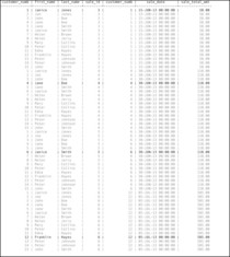
A projection of a relation is a new relation created by copying one or more the columns from the original relation into a new table. As an example, consider Figure 2-1. The result table (arbitrarily called Names_and_numbers) is a projection of the customer relation with the attributes customer_numb, first_name, and last_name.
 |
| Figure 2-1 Taking a projection |
Using the syntax for relational algebra, the projection in Figure 2-1 is written:
PROJECT customer_rows, first_name, last_name
FROM customer GIVING Names_and_numbers
The order of the columns in the result table is based on the order in which the column names appear in the project statement; the order in which they are defined in the source table has no effect on the result. Rows appear in the order in which they are stored in the source table; project does not include sorting or ordering the data in any way. As with all relational algebra operations, duplicate rows are removed.
Note: It is important to keep in mind that relational algebra is first and foremost a set of theoretical operations. A DBMS may not implement an operation the same way that it is described in theory. For example, most DBMSs don't remove duplicate rows from result tables unless the user requests it explicitly. Why? Because to remove duplicates the DBMS must sort the result table by every column (so that duplicate rows will be next to one another) and then scan the table from top to bottom looking for the duplicates. This can be a very slow process if the result table is large.
Whenever you issue a SQL command that asks for specific columns—just about every retrieval command—you are asking the DBMS to perform the project operation. Project is a very fast operation because the DBMS does not need to evaluate any of the data in the table.
There is one issue with project with which you need to be concerned. A DBMS will project any columns that you request. It makes no judgment as to whether the selected columns produce a meaningful result. For example, consider the following operation:
PROJECT sale_total_amt, exp_month FROM sale GIVING invalid
In theory, there is absolutely nothing wrong with this project. However, it probably doesn't mean much to associate a dollar amount with a credit card expiration month. Notice in Figure 2-2 that because there is more than one sale with the same total cost (for example, $110), the same sale value is associated with more than one expiration month. We could create a concatenated primary key for the result table using both columns, but that still wouldn't make the resulting table meaningful in the context of the database environment. There is no set of rules as to what constitutes a meaningful projection. Judgments as to the usefulness of projections depend solely on the meaning of the data the database is trying to capture.
 |
| Figure 2-2 An invalid projection |
Making Horizontal Subsets: Restrict
The restrict operation asks a DBMS to choose rows that meet some logical criteria. As defined in the relational algebra, restrict copies rows from the source relation into a result table. Restrict copies all attributes; it has no way to specify which attributes should be included in the result table.
Restrict identifies which rows are to be included in the result table with a logical expression known as a predicate. The operation therefore takes the following general form:
RESTRICT FROM source_table_name WHERE predicate GIVING result_table_name
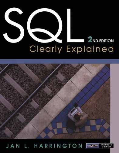
For example, suppose we want to retrieve data about customers who live in zipcode 11111. The operation might be expressed as
RESTRICT FROM customer WHERE zip_postcode = ‘11111’ GIVING one_zip
The result appears in Figure 2-3. The result table includes the entire row for each customer that has a value of 11111 in the zip_postcode column.
Note: There are many operators that can be used to create a restrict predicate, some of which are unique to SQL. You will begin to read about constructing predicates inChapter 4.
 |
| Figure 2-3 Restricting rows from a relation |
Choosing Columns and Rows: Restrict and Then Project
As we said at the beginning of this chapter, most SQL queries require more than one relational algebra operation. We might, for example, want to see just the names of the customers that live in zipcode 11111. Because such a query requires both a restrict and a project, it takes two steps:
1. Restrict the rows to those with customers that live in zipcode 1111.
2. Project the first and last name columns.
In some cases the order of the restrict and project may not matter. However, in this particular example the restrict must be performed first. Why? Because the project removes the column needed for the restrict predicate from the intermediate result table, which would make it impossible to perform the restrict.
It is up to a DBMS to determine the order in which it will perform relational algebra operations to obtain a requested result. A query optimizer takes care of making the decisions. When more than one series of operations will generate the same result, the query optimizer attempts to determine which will provide the best performance and will then execute that strategy.
Note: There is a major tradeoff for a DBMS when it comes to query optimization. Picking the most efficient query strategy can result in the shortest query execution time, but it is also possible for the DBMS to spend so much time figuring out which strategy is best that it consumes any performance advantage that might be had by executing the best strategy. Therefore, the query strategy used by a DBMS may not be the theoretically most efficient strategy, but it is the most efficient strategy that can be identified relatively quickly.
Unoin
The union operation creates a new table by placing all rows from two source tables into a single result table, placing the rows on top of one another. As an example of how a union works, assume that you have the two tables at the top of Figure 2-4. The operation produces the result table at the bottom of Figure 2-4.
in_print_books UNION out_of_print_books GIVING union_result
 |
| Figure 2-4 Thee union operation |
For a union operation to be possible, the two source tables must be union compatible. In the relational algebra sense, this means that their columns must be defined over the same domains. The tables must have the same columns, but the columns do not necessarily need to be in the same order or be the same size.
In practice, however, the rules for union compatibility are stricter. The two source tables on which the union is performed must have columns with the same data types and sizes, in the same order. As you will see, in SQL the two source tables are actually virtual tables created by two independent retrieval statements, which are then combined by the union operation.
Join
Join is arguably the most useful relational algebra operations because it combines two tables into one, usually via a primary key-foreign key relationship. Unfortunately, a join can also be an enormous drain on database performance.
A Non-Database Example
To help you understand how a join works, we will begin with an example that has absolutely nothing to do with relations. Assume that you have been given the task of creating manufacturing part assemblies by connecting two individual parts. The parts are classified as either A parts or B parts.
There are many types of A parts (A1 through An, where n is the total number of types of A parts) and many types of B parts (B1 through Bn). Each B is to be matched to the A part with the same number; conversely, an A part is to be matched to a B part with the same number.
The assembly process requires four bins. One contains the A parts, one contains the B parts, and one will hold the completed assemblies. The remaining bin will hold parts that cannot be matched. (The unmatched parts bin is not strictly necessary; it is simply for your convenience.)
You begin by extracting a part from the B bin. You look at the part to determine the A part to which it should be connected. Then, you search the A bin for the correct part. If you can find a matching A part, you connect the two pieces and toss them into the completed assemblies bin. If you cannot find a matching A part, then you toss the unmatched B part into the bin that holds unmatched B parts. You repeat this process until the B bin is empty. Any unmatched A parts will be left in their original location.
Note: You could just as easily have started with the bin containing the A parts. The contents of the bin holding the completed assemblies will be the same.
As you might guess, the A bins and B bins are analogous to tables that have a primary to foreign key relationships. This matching of part numbers is very much like the matching of data that occurs when you perform a join. The completed assembly bin corresponds to the result table of the operation. As you read about the operation of a join, keep in mind that the parts that could not be matched were left out of the completed assemblies bin.
The Equi-Join
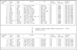
In its most common form, a join forms new rows when data in the two source tables match. Because we are looking for rows with equal values, this type of join is known as an equi-join (or a natural equi-join). It is also often called an inner join. As an example, consider the join in Figure 2-5.
 |
| Figure 2-5 An equi-join |
Notice that the customer_numb column is the primary key of the customer_data table and that the same column is a foreign key in the sale_data table. The customer_numb column in sale_data therefore serves to relate sales to the customers to which they belong.
Assume that you want to see the names of the customers who placed each order. To do so, you must join the two tables, creating combined rows wherever there is a matching customer_ numb. In database terminology, we are joining the two tables over customer_numb. The result table, joined_table, can be found at the bottom of Figure 2-5.
An equi-join can begin with either source table. (The result should be the same regardless of the direction in which the join is performed.) The join compares each row in one source table with the rows in the second. For each row in the first source table that matches data in the second source table in the column or columns over which the join is being performed, a new row is placed in the result table.
Assume that we are using the customer_data table as the first source table, producing the result table in Figure 2-5 might therefore proceed conceptually as follows:
1. Search sale_data for rows with a customer_numb of 1. There are four matching rows in sale_data. Create four new rows in the result table, placing the same customer information in each row along with the data from sale_data.
2. Search sale_data for rows with a customer_numb of 2. Because there are three rows for customer 2 in sale_ data, add three rows to the result table.
3. Search sale_data for rows with a customer_numb of 3. Because there are no matching rows in sale_data, do not place a row in the result table.
4. Continue as established until all rows from customer_ data have been compared to sale_data.
If the customer_numb column does not appear in both tables, then no row is placed in the result table. This behavior categorizes this type of join as an inner join. (Yes, there is such a thing as an outer join. You will read about it shortly.)
What's Really Going On: Product and Restrict
From a relational algebra point of view, a join can be implemented using two other operations: product and restrict. As you will see, this sequence of operations requires the manipulation of a great deal of data and, if implemented by a DBMS, can result in slow query performance. Many of today's DBMSs therefore use alternative techniques for processing joins. None-theless, the concept of using product followed by restrict underlies the original SQL join syntax.
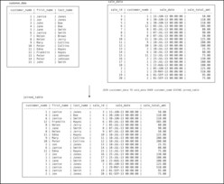
The product operation (the mathematical Cartesian product) makes every possible pairing of rows from two source tables. The product of the tables in Figure 2-5 produces a result table with 300 rows (the 15 rows in customer_data times the 20 rows in sale_data), the first 60 of which appear in Figure 2-6.
Note: Although 300 rows may not seem like a lot, consider the size of a product table created from tables with 10,000 and 100,000 rows! The manipulation of a table of this size can tie up a lot of disk I/O and CPU time.
 |
| Figure 2-6 The first 60 rows of a 300 row product table |
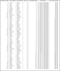
Notice first that the customer_numb is included twice in the result table, once from each source table. Second, notice that in some rows, the customer_numb is the same. These are the rows that would have been included in a join. We can therefore apply a restrict predicate (a join condition) to the product table to end up with same table provided by the join you saw earlier. The predicate can be written:
customer.customer_numb = sale.customer_numb
The rows that are selected by this predicate from the first 60 rows in the product table appear in black in Figure 2-7; those eliminated by the predicate are gray.
Note: The “dot notation” that you see in the preceding join condition is used throughout SQL. The table name is followed by a dot, which is followed by the column name. This makes it possible to have the same column name in more than one table and yet be able to distinguish among them.
 |
| Figure 2-7 The four rows of the product in Figure 2-6 that are returned by the join condition in a restrict predicate |
It is important that you keep in mind the implication of this sequence to two relational algebra operations when you are writing SQL joins. If you are using the traditional SQL syntax for a join (the first join syntax we'll be discussing) and you forget the predicate for the join condition, you will end up with a product. The product table contains bad information; it implies facts that are not actually stored in the database. It is therefore potentially harmful, in that a user who does not understand how the result table came to be might assume that it is correct and make business decision based on the bad data.
Equi-Joins over Concatenated Keys
The joins you have seen so far have used a single-column primary key and a single-column foreign key. There is no reason, however, that the values used in a join can't be concatenated. As an example, let's look again at the accounting firm example from Chapter 1. The design of the portion of the database that we used was
accountant (acct_first_name, acct_last_name, date_hired, office_ext)
customer (customer_numb, first_name, last_name, street, city, state_province, zip_postcode, contact_phone)
project (tax_year, customer_numb, acct_first_name, acct_last_name)
form (tax_year, customer_numb, form_id, is_complete)
Suppose we want to see all the forms and the year that the forms were completed for the customer named Peter Jones by the accountant named Edgar Smith. The sequence of relational operations would go something like this:
1. Restrict from the customer table to find the single row for Peter Jones. Because some customers have duplicated names, the restrict predicate would probably contain the name and the phone number.
2. Join the table created in Step 1 to the project table over the customer number.
3. Restrict from the table created in Step 2 to find the projects for Peter Jones that were handled by the accountant Edgar Smith.
4. Now we need to get the data about which forms appear on the projects identified in Step 3. We therefore need to join the table created in Step 3 to the form table. The foreign key in the form table is the concatenation of the tax year and customer number, which just happens to match the primary key of the project table. The join is therefore over the concatenation of the tax year and customer number rather than over the individual values. When making its determination whether to include a row in the result table, the DBMS puts the tax year and customer number together for each row and treats the combined value as if it were one.
5. Project the tax year and form ID to present the specific data requested in the query.
To see why treating a concatenated foreign key as a single unit when comparing to a concatenated foreign key is required, take a look at Figure 2-8. The two tables at the top of the illustration are the original project and form tables created for this example. We are interested in customer number 18 (our friend Peter Jones), who has had projects handled by Edgar Smith in 2006 and 2007.
 |
 |
| Figure 2-8 Joining using concatenated keys |
Result table (a) is what happens if you join the tables (without restricting for customer 18) only over the tax year. This invalid join expands the 10 row form table to 20 rows. The data imply that the same customer had the same form prepared by more than one accountant in the same year.
Result table (b) is the result of joining the two tables just over the customer number. This time the invalid result table implies that in some cases the same form was completed in two years.
The correct join appears in result table (c) in Figure 2-8. It has the correct 10 rows, one for each form. Notice that both the tax year and customer number are the same in each row, as we intended them to be.
Note: The examples you have seen so far involve two concatenated columns. There is no reason, however, that the concatenation cannot involve more than two columns if necessary.
Θ-Joins
An equi-join is a specific example of a more general class of join known as a Θ-join (theta-join). A Θ-join combines two tables on some condition, which may be equality or may be something else. To make it easier to understand why you might want to join on something other than equality and how such joins work, assume that you're on vacation at a resort that offers both biking and hiking. Each outing runs a half day, but the times at which the outings start and end differ. The tables that hold the outing schedules appear in Figure 2-9. As you look at the data, you'll see that some ending and starting times overlap, which means that if you want to engage in two outings on the same day, only some pairings of hiking and biking will work.
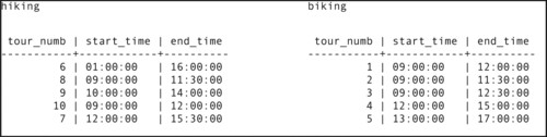 |
| Figure 2-9 Source tables for the θ-join examples |
To determine which pairs of outings you could do on the same day, you need to find pairs of outings that satisfy either of the following conditions:
hiking.end_time < biking.start_time
biking.end_time < hiking.start_time
A Θ-join over either of those conditions will do the trick, producing the result tables in Figure 2-10. The top result table contains pairs of outings where hiking is done first; the middle result table contains pairs of outings where biking is done first. If you want all the possibilities in the same table, a union operation will combine them, as in the bottom result table. Another way to generate the combined table is to use a complex join condition in the Θ-join:
hiking.end_time < biking.start_time OR biking.end_time < hiking.start_time
Note: As with the more restrictive equi-join, the “start” table for a θ-join does not matter. The result will be the same either way.
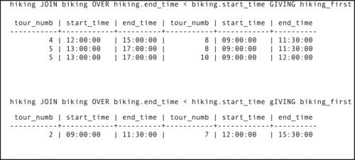 |
| Figure 2-10 The results of θ-joins of the tables in Figure 2-9 |
Outer Joins
An outer join (as opposed to the inner joins we have been considering so far) is a join that includes rows in a result table even though there may not be a match between rows in the two tables being joined. Wherever the DBMS can't match rows, it places nulls in the columns for which no data exist. The result may therefore not be a legal relation, because it may not have a primary key. However, because the query's result table is a virtual table that is never stored in the database, having no primary key does not present a data integrity problem.
Why might someone want to perform an outer join? An employee of the rare book store, for example, might want to see the names of all customers along with the books ordered in the last week. An inner join of customer to sale would eliminate those customers who had not purchased anything during the previous week. However, an outer join will include all customers, placing nulls in the sale data columns for the customers who have not ordered. An outer join therefore not only shows you matching data but also tells you where matching data do not exist.
There are really three types of outer join, which vary depending the table or tables from which you want to include rows that have no matches.
The Left Outer Join
The left outer join includes all rows from the first table in the join expression
Table1 LEFT OUTER JOIN table2 GIVING result_table
For example, if we use the data from the tables in Figure 2-5 and perform the left outer join asthen the result will appear as in Figure 2-11: There is a row for every row in customer. For the rows that don't have orders, the columns that come from sale have been filled with nulls.
customer LEFT OUTER JOIN sale GIVING left_outer_join_result
 |
| Figure 2-11 The result of a left outer join |
The Right Outer Join
The right outer join is the precise opposite of the left outer join. It includes all rows from the table on the right of the outer join operator. If you perform using the data from Figure 2-5, the result will be the same as an inner join of the two tables. This occurs because there are no rows in sale that don't appear in customer. However, if you reverse the order of the tables, as inyou end up with the same data as Figure 2-11.
customer RIGHT OUTER JOIN sale GIVING right_outer_join_result
sale RIGHT OUTER JOIN customer GIVING right_outer_join_result
Choosing a Right versus Left Outer Join
As you have just read, outer joins are directional: the result depends on the order of the tables in the command. (This is in direct contrast to an inner join, which produces the same result regardless of the order of the tables.) Assuming that you are performing an outer join on two tables that have a primary key-foreign key relationship, then the result of left and right outer joins on those tables is predictable (see Table 2-1). Referential integrity ensures that no rows from a table containing a foreign key will ever be omitted from a join with the table that contains the referenced primary key. Therefore, a left outer join where the foreign key table is on the left of the operator and a right outer join where the foreign key table is on the right of the operator are no different from an inner join.
The Full Outer Join
When choosing between a left and a right outer join, you therefore need to pay attention to which table will appear on which side of the operator. If the outer join is to produce a result different from that of an inner join, then the table containing the primary key must appear on the side that matches the name of the operator.
A full outer join includes all rows from both tables, filling in rows with nulls where necessary. If the two tables have a primary key-foreign key relationship, then the result will be the same as that of either a left outer join when the primary key table is on the left of the operator or a right outer join when the primary key table is on the right side of the operator. In the case of the full outer join, it does not matter on which side of the operator the primary key table appears; all rows from the primary key table will be retained.
Valid versus Invalid Joins
To this point, all of the joins you have seen have involved tables with a primary key-foreign key relationship. These are the most typical types of join and always produce valid result tables. In contrast, most joins between tables that do not have a primary key-foreign key relationship are not valid. This means that the result tables contain information that is not represented in the database, conveying misinformation to the user. Invalid joins are therefore far more dangerous than meaningless projections.
As an example, let's temporarily add a table to the rare book store database. The purpose of the table is to indicate the source from which the store acquired a volume. Over time, the same book (different volumes) may come from more than one source. The table has the following structure:
book_sources (isbn, source_name)
Someone looking at this table and the book table might conclude that because the two tables have a matching column (isbn) it makes sense to join the tables to find out the source of every volume that the store has ever had in inventory. Unfortunately, this is not the information that the result table will contain.
To keep the result table to a reasonable length, we'll work with an abbreviated book_sources table that doesn't contain sources for all volumes (Figure 2-12). Let's assume that we go ahead and join the tables over the ISBN. The result table (without columns that aren't of interest to the join itself) can be found in Figure 2-13.
 |
| Figure 2-12 The book_sources table |
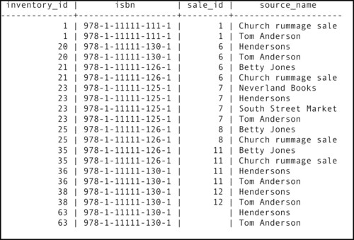 |
| Figure 2-13 An invalid join result |
If the store has ever obtained volumes with the same ISBN from different sources, there will be multiple rows for that ISBN in the book_sources table. Although this doesn't give us a great deal of meaningful information, in and of itself the table is valid. However, when we look at the result of the join with the volume table, the data in the result table contradict what is in book_sources. For example, the first two rows in the result table have the same inventory ID number, yet come from different sources. How can the same volume come from two places? That is physically impossible. This invalid join therefore implies facts that simply cannot be true.
The reason this join is invalid is that the two columns over which the join is performed are not in a primary key-foreign key relationship. In fact, in both tables the isbn column is a foreign key that references the primary key of the book table.
Are joins between tables that do not have a primary key-foreign key relationship ever valid? On occasion, they are, in particular if you are joining two tables with the same primary key. You will see an example of this type of join when we discuss joining a table to itself when a predicate requires that multiple rows exist before any are placed in a result table.
For another example, assume that you want to create a table to store data about your employees:
employees (id_numb, first_name, last_name, department, job_title, salary, hire_date)
Some of the employees are managers. For those individuals, you also want to store data about the project they are currently managing and the date they began managing that project. (A manager handles only one project at a time.) You could add the columns to the employees table and let them contain nulls for employees who are not managers. An alternative is to create a second table just for the managers:
managers (id_numb, current_project, project_start_date)
When you want to see all the information about a manager, you must join the two tables over the id_numb column. The result table will contain rows only for the manager because employees without rows in the managers table will be left out of the join. There will be no spurious rows such as those we got when we joined the volume and book_sources tables. This join therefore is valid.
Note: Although the id_numb column in the managers table technically is not a foreign key referencing employees, most data-bases using such a design would nonetheless include a constraint that forced the presence of a matching row in employees for every manager.
The bottom line is that you need to be very careful when performing joins between tables that do not have a primary keyforeign key relationship. Although such joins are not always invalid, in most cases they will be.
Difference
Among the most powerful database queries are those phrased in the negative, such as “show me all the customers who have not purchased from us in the past year.” This type of query is particularly tricky because it asking for data that are not in the database. The rare book store has data about customers who have purchased, but not those who have not. The only way to perform such a query is to request the DBMS to use the difference operation.
Difference retrieves all rows that are in one table but not in another. For example, if you have a table that contains all your products and another that contains products that have been purchased the expression—
all_products MINUS products_that_have_been_purchased GIVING not_purchased
—is the products that have not been purchased. When you remove the products that have been purchased from all products, what are left are the products that have not been purchased.
The difference operation looks at entire rows when it makes the decision whether to include a row in the result table. This means that the two source tables must be union compatible. Assume that the all_products table has two columns—prod_numb and product_name—and the products_that_have_been_ purchased table also has two columns—prod_numb and order_ numb. Because they don't have the same columns, the tables aren't union-compatible.
As you can see from Figure 2-14, this means that a DBMS must first perform two projections to generate the union-compatible tables before it can perform the difference. In this case, the operation needs to retain the product number. Once the projections into union-compatible tables exist, the DBMS can perform the difference.
 |
| Figure 2-14 The difference operation |
Intersect
As mentioned earlier in this chapter, to be considered relationally complete a DBMS must support restrict, project, join, union, and difference. Virtually every query can be satisfied using a sequence of those five operations. However, one other operation is usually included in the relational algebra specification: intersect.
In one sense, the intersect operation is the opposite of union. Union produces a result containing all rows that appear in either relation, while intersect produces a result containing all rows that appear in both relations. Intersection can therefore only be performed on two union-compatible relations.
Assume, for example, that the rare book store receives data listing volumes in a private collection that are being offered for sale. We can find out which volumes are already in the store's inventory using an intersect operation:
books_in_inventory INTERSECT books_for_sale GIVING already_have
As you can see in Figure 2-15, the first step in the process is to use the project operation to create union-compatible operations. Then an intersect will provide the required result. (Columns that are not a part of the operation have been omitted so that the tables will fit on the book page.)
Note: A join over the concatenation of all the columns in the two tables produces the same result as an intersect.
 |
| Figure 2-15 The intersect operation |
Divide
An eighth relational algebra operation—divide—is often included with the operations you have seen in this chapter. It can be used for queries that need to have multiple rows in the same source table for a row to be included in the result table. Assume, for example, that the rare book store wants a list of sales on which two specific volumes have appeared.
There are many forms of the divide operation, all of which except the simplest are extremely complex. To set up the simplest form you need two relations, one with two columns (a binary relation) and one with a single column (a unary relation). The binary relation has a column that contains the values that will be placed in the result of the query (in our example, a sale ID) and a column for the values to be queried (in our example, the ISBN of the volume). This relation is created by taking a projection from the source table (in this case, the volume table).
The unary relation has the column being queried (the ISBN). It is loaded with a row for each value that must be matched in the binary table. A sale ID will be placed in the result table for all sales that contain ISBNs that match all of the values in the unary table. If there are two ISBNs in the unary table, then there must be a row for each of them with the same sale ID in the binary table to include the sale ID in the result. If we were to load the unary table with three ISBNs, then three matching rows would be required.
You can get the same result as a divide using multiple restricts and joins. In our example, you would restrict the volume table twice, once for the first ISBN and once for the second. Then you would join the tables over the sale ID. Only those sales that had rows in both of the tables being joined would end up in the result table.
Because divide can be performed fairly easily with restrict and join, DBMSs generally do not implement it directly.
..................Content has been hidden....................
You can't read the all page of ebook, please click here login for view all page.