Chapter 10

Zeroing In on the Data You Want

In This Chapter

Specifying the tables you want to work with

Separating rows of interest from the rest

Building effective WHERE clauses

Handling null values

Building compound expressions with logical connectives

Grouping query output by column

Putting query output in order

Operating on related rows

A database management system has two main functions: storing data and providing easy access to that data. Storing data is nothing special; a file cabinet can perform that chore. The hard part of data management is providing easy access. For data to be useful, you must be able to separate the (usually) small amount you want from the huge amount you don’t want.

SQL enables you to use some characteristics of the data to determine whether a particular table row is of interest to you. The SELECT, DELETE, and UPDATE statements convey to the database engine (the part of the DBMS that interacts directly with the data), which rows to select, delete, or update. You add modifying clauses to the SELECT, DELETE, and UPDATE statements to refine the search to your specifications.

Modifying Clauses

The modifying clauses available in SQL are FROM, WHERE, HAVING, GROUP BY, and ORDER BY. The FROM clause tells the database engine which table or tables to operate on. The WHERE and HAVING clauses specify a data characteristic that determines whether or not to include a particular row in the current operation. The GROUP BY and ORDER BY clauses specify how to display the retrieved rows. Table 10-1 provides a summary.

Table 10-1 Modifying Clauses and Functions

Modifying Clause	Function
FROM	Specifies from which tables data should be taken
WHERE	Filters out rows that don’t satisfy the search condition
GROUP BY	Separates rows into groups based on the values in the grouping columns
HAVING	Filters out groups that don’t satisfy the search condition
ORDER BY	Sorts the results of prior clauses to produce final output

If you use more than one of these clauses, they must appear in the following order:

SELECT column_list

   FROM table_list

   [WHERE search_condition]

   [GROUP BY grouping_column]

   [HAVING search_condition]

   [ORDER BY ordering_condition] ;

Here’s the lowdown on the execution of these clauses:

The WHERE clause is a filter that passes the rows that meet the search condition and rejects rows that don't meet the condition.

The GROUP BY clause rearranges the rows that the WHERE clause passes according to the value of the grouping column.

The HAVING clause is another filter that takes each group that the GROUP BY clause forms and passes those groups that meet the search condition, rejecting the rest.

The ORDER BY clause sorts whatever remains after all the preceding clauses process the table.

As the square brackets ([ ]) indicate, the WHERE, GROUP BY, HAVING, and ORDER BY clauses are optional.

SQL evaluates these clauses in the order FROM, WHERE, GROUP BY, HAVING, and finally SELECT. The clauses operate like a pipeline — each clause receives the result of the prior clause and produces an output for the next clause. In functional notation, this order of evaluation appears as follows:

SELECT(HAVING(GROUP BY(WHERE(FROM...))))

ORDER BY operates after SELECT, which explains why ORDER BY can only reference columns in the SELECT list. ORDER BY can't reference other columns in the FROM table(s).

FROM Clauses

The FROM clause is easy to understand if you specify only one table, as in the following example:

SELECT * FROM SALES ;

This statement returns all the data in all the rows of every column in the SALES table. You can, however, specify more than one table in a FROM clause. Consider the following example:

SELECT *

   FROM CUSTOMER, SALES ;

This statement forms a virtual table that combines the data from the CUSTOMER table with the data from the SALES table. (For more about virtual tables, see Chapter 6.) Each row in the CUSTOMER table combines with every row in the SALES table to form the new table. The new virtual table that this combination forms contains the number of rows in the CUSTOMER table multiplied by the number of rows in the SALES table. If the CUSTOMER table has 10 rows and the SALES table has 100, then the new virtual table has 1,000 rows.

This operation is called the Cartesian product of the two source tables. The Cartesian product is a type of JOIN. (I cover JOIN operations in detail in Chapter 11.)

In most applications, when you take the Cartesian product of two tables, most of the rows that are formed in the new virtual table are meaningless. That's also true of the virtual table that forms from the CUSTOMER and SALES tables; only the rows where the CustomerID from the CUSTOMER table matches the CustomerID from the SALES table are of interest. You can filter out the rest of the rows by using a WHERE clause.

WHERE Clauses

I use the WHERE clause many times throughout this book without really explaining it because its meaning and use are obvious: A statement performs an operation (such as SELECT, DELETE, or UPDATE) only on table rows WHERE a stated condition is True. The syntax of the WHERE clause is as follows:

SELECT column_list

   FROM table_name

   WHERE condition ;

 

DELETE FROM table_name

   WHERE condition ;

 

UPDATE table_name

   SET column1=value1, column2=value2, ..., columnn=valuen

   WHERE condition ;

The condition in the WHERE clause may be simple or arbitrarily complex. You may join multiple conditions together by using the logical connectives AND, OR, and NOT (which I discuss later in this chapter) to create a single condition.

The following are some typical examples of WHERE clauses:

WHERE CUSTOMER.CustomerID = SALES.CustomerID

WHERE FOODS.Calories = COMIDA.Caloria

WHERE FOODS.Calories < 219

WHERE FOODS.Calories > 3 * base_value

WHERE FOODS.Calories < 219 AND FOODS.Protein > 27.4

The conditions that these WHERE clauses express are known as predicates. A predicate is an expression that asserts a fact about values.

The predicate FOODS.Calories < 219, for example, is True if the value for the current row of the column FOODS.Calories is less than 219. If the assertion is True, it satisfies the condition. An assertion may be True, False, or unknown. The unknown case arises if one or more elements in the assertion are null. The comparison predicates (=, <, >, <>, <=, and >=) are the most common, but SQL offers several others that greatly increase your capability to filter out a desired data item from others in the same column. These predicates give you that filtering capability:

Comparison predicates

BETWEEN

IN [NOT IN]

LIKE [NOT LIKE]

NULL

ALL, SOME, ANY

EXISTS

UNIQUE

OVERLAPS

MATCH

SIMILAR

DISTINCT

Comparison predicates

The examples in the preceding section show typical uses of comparison predicates in which you compare one value withanother. For every row in which the comparison evaluates to a True value, that value satisfies the WHERE clause, and the operation (SELECT, UPDATE, DELETE, or whatever) executes upon that row. Rows that the comparison evaluates to FALSE are skipped. Consider the following SQL statement:

SELECT * FROM FOODS

   WHERE Calories <219 ;

This statement displays all rows from the FOODS table that have a value of less than 219 in the Calories column.

Six comparison predicates are listed in Table 10-2.

Table 10-2 SQL’s Comparison Predicates

Comparison	Symbol
Equal	=
Not equal	<>
Less than	<
Less than or equal	<=
Greater than	>
Greater than or equal	>=

BETWEEN

Sometimes you want to select a row if the value in a column falls within a specified range. One way to make this selection is by using comparison predicates. For example, you can formulate a WHERE clause to select all the rows in the FOODS table that have a value in the Calories column greater than 100 and less than 300, as follows:

WHERE FOODS.Calories > 100 AND FOODS.Calories < 300

This comparison doesn’t include foods with a calorie count of exactly 100 or 300 — only those values that fall between these two numbers. To include the end points (in this case, 100 and 300), you can write the statement as follows:

WHERE FOODS.Calories >= 100 AND FOODS.Calories <= 300

Another way of specifying a range that includes the end points is to use a BETWEEN predicate in the following manner:

WHERE FOODS.Calories BETWEEN 100 AND 300

This clause is functionally identical to the preceding example, which uses comparison predicates. This formulation saves some typing — and it's a little more intuitive than the one that uses two comparison predicates joined by the logical connective AND.

The BETWEEN keyword may be confusing because it doesn't tell you explicitly whether the clause includes the end points. In fact, the clause does include these end points. When you use the BETWEEN keyword, a little birdy doesn't swoop down to remind you that the first term in the comparison must be equal to or less than the second. If, for example, FOODS.Calories contains a value of 200, the following clause returns a True value:

WHERE FOODS.Calories BETWEEN 100 AND 300

However, a clause that you may think is equivalent to the preceding example returns the opposite result, False:

WHERE FOODS.Calories BETWEEN 300 AND 100

If you use BETWEEN, you must be able to guarantee that the first term in your comparison is always equal to or less than the second term.

You can use the BETWEEN predicate with character, bit, and datetime data types as well as with the numeric types. You may see something like the following example:

SELECT FirstName, LastName

   FROM CUSTOMER

   WHERE CUSTOMER.LastName BETWEEN 'A' AND 'Mzzz' ;

This example returns all customers whose last names are in the first half of the alphabet.

IN and NOT IN

The IN and NOT IN predicates deal with whether specified values (such as OR, WA, and ID) are contained within a particular set of values (such as the states of the United States). You may, for example, have a table that lists suppliers of a commodity that your company purchases on a regular basis. You want to know the phone numbers of the suppliers located in the Pacific Northwest. You can find these numbers by using comparison predicates, such as those shown in the following example:

SELECT Company, Phone

   FROM SUPPLIER

   WHERE State = 'OR' OR State = 'WA' OR State = 'ID' ;

You can also use the IN predicate to perform the same task, as follows:

SELECT Company, Phone

   FROM SUPPLIER

   WHERE State IN ('OR', 'WA', 'ID') ;

This formulation is a bit more compact than the one using comparison predicates and logical OR. It also eliminates any possible confusion between the logical OR operator and the abbreviation for the state of Oregon.

The NOT IN version of this predicate works the same way. Say that you have locations in California, Arizona, and New Mexico, and to avoid paying sales tax, you want to consider using suppliers located anywhere except in those states. Use the following construction:

SELECT Company, Phone

   FROM SUPPLIER

   WHERE State NOT IN ('CA', 'AZ', 'NM') ;

Using the IN keyword this way saves you a little typing — though (frankly) that isn't much of an advantage. You can do the same job by using comparison predicates as shown in this section's first example.

You may have another good reason to use the IN predicate rather than comparison predicates, even if using IN doesn't save much typing: Your DBMS probably implements the two methods differently, and one of the methods may be significantly faster than the other on your system. You may want to run a performance comparison on the two ways of expressing inclusion in (or exclusion from) a group and then use the technique that produces the quicker result. A DBMS with a good optimizer will probably choose the more efficient method, regardless of which predicate you use.

The IN keyword is valuable in another area, too. If IN is part of a subquery, the keyword enables you to pull information from two tables to obtain results that you can't derive from a single table. I cover subqueries in detail in Chapter 12, but here's an example that shows how a subquery uses the IN keyword.

Suppose you want to display the names of all customers who’ve bought the F-35 product in the last 30 days. Customer names are in the CUSTOMER table, and sales transaction data is in the TRANSACT table. You can use the following query:

SELECT FirstName, LastName

   FROM CUSTOMER

   WHERE CustomerID IN

      (SELECT CustomerID

         FROM TRANSACT

         WHERE ProductID = 'F-35'

         AND TransDate >= (CurrentDate - 30)) ;

The inner SELECT of the TRANSACT table nests within the outer SELECT of the CUSTOMER table. The inner SELECT finds the CustomerID numbers of all customers who bought the F-35 product in the last 30 days. The outer SELECT displays the first and last names of all customers whose CustomerID is retrieved by the inner SELECT.

LIKE and NOT LIKE

You can use the LIKE predicate to compare two character strings for a partial match. Partial matches are valuable if you don't know the exact form of the string for which you're searching. You can also use partial matches to retrieve multiple rows that contain similar strings in one of the table's columns.

To identify partial matches, SQL uses two wildcard characters. The percent sign (%) can stand for any string of characters that have zero or more characters. The underscore (_) stands for any single character. Table 10-3 provides some examples that show how to use LIKE.

Table 10-3 SQL’s LIKE Predicate

Statement	Values Returned
WHERE Word LIKE 'intern%'	intern
	internal
	international
	internet
	interns
WHERE Word LIKE '%Peace%'	Justice of the Peace
	Peaceful Warrior
WHERE Word LIKE 'T_p_'	Tape
	Taps
	Tipi
	Tips
	Tops
	Type

The NOT LIKE predicate retrieves all rows that don't satisfy a partial match, including one or more wildcard characters, as in the following example:

WHERE Phone NOT LIKE '503%'

This example returns all the rows in the table for which the phone number starts with something other than 503.

You may want to search for a string that includes an actual percent sign or underscore. In that case, you want SQL to interpret the percent sign as a percent sign and not as a wildcard character. You can conduct such a search by typing an escape character just prior to the character you want SQL to take literally. You can choose any character as the escape character as long as that character doesn’t appear in the string that you’re testing, as shown in the following example:

SELECT Quote

   FROM BARTLETTS

   WHERE Quote LIKE '20#%'

      ESCAPE '#' ;

The % character is escaped by the preceding # sign, so the statement interprets this symbol as a percent sign rather than as a wildcard. You can "escape" an underscore — or the escape character itself — in the same way. The preceding query, for example, would find the following quotation in Bartlett's Familiar Quotations:

20% of the salespeople produce 80% of the results.

The query would also find the following:

20%

SIMILAR

SQL:1999 added the SIMILAR predicate, which offers a more powerful way of finding partial matches than the LIKE predicate provides. With the SIMILAR predicate, you can compare a character string to a regular expression. For example, say you're searching the OperatingSystem column of a software compatibility table to look for Microsoft Windows compatibility. You could construct a WHERE clause such as the following:

WHERE OperatingSystem SIMILAR TO

'('Windows '(3.1|95|98|ME|CE|NT|2000|XP|Vista|7|8))'

This predicate retrieves all rows that contain any of the specified Microsoft operating systems.

NULL

The NULL predicate finds all rows where the value in the selected column is null. In the FOODS table in Chapter 8, several rows have null values in the Carbohydrate column. You can retrieve their names by using a statement such as the following:

SELECT (Food)

   FROM FOODS

   WHERE Carbohydrate IS NULL ;

This query returns the following values:

Beef, lean hamburger

Chicken, light meat

Opossum, roasted

Pork, ham

As you might expect, including the NOT keyword reverses the result, as in the following example:

SELECT (Food)

   FROM FOODS

   WHERE Carbohydrate IS NOT NULL ;

This query returns all the rows in the table except the four that the preceding query returns.

The statement Carbohydrate IS NULL is not the same as Carbohydrate = NULL. To illustrate this point, assume that, in the current row of the FOODS table, both Carbohydrate and Protein are null. From this fact, you can draw the following conclusions:

Carbohydrate IS NULL is True.

Protein IS NULL is True.

Carbohydrate IS NULL AND Protein IS NULL is True.

Carbohydrate = Protein is unknown.

Carbohydrate = NULL is an illegal expression.

Using the keyword NULL in a comparison is meaningless because the answer always returns as unknown.

Why is Carbohydrate = Protein defined as unknown even though Carbohydrate and Protein have the same (null) value? Because NULL simply means "I don't know." You don't know what Carbohydrate is, and you don't know what Protein is; therefore you don't know whether those (unknown) values are the same. Maybe Carbohydrate is 37, and Protein is 14, or maybe Carbohydrate is 93, and Protein is 93. If you don't know both the carbohydrate value and the protein value, you can't say whether the two are the same.

ALL, SOME, ANY

Thousands of years ago, the Greek philosopher Aristotle formulated a system of logic that became the basis for much of Western thought. The essence of this logic is to start with a set of premises that you know to be true, apply valid operations to these premises, and, thereby, arrive at new truths. An example of this procedure is as follows:

Premise 1: All Greeks are human.

Premise 2: All humans are mortal.

Conclusion: All Greeks are mortal.

Another example:

Premise 1: Some Greeks are women.

Premise 2: All women are human.

Conclusion: Some Greeks are human.

By way of presenting a third example, let me state the same logical idea of the second example in a slightly different way:

If any Greeks are women and all women are human, then some Greeks are human.

The first example uses the universal quantifier ALL in both premises, enabling you to make a sound deduction about all Greeks in the conclusion. The second example uses the existential quantifier SOME in one premise, enabling you to make a deduction about some Greeks in the conclusion. The third example uses the existential quantifier ANY, which is a synonym for SOME, to reach the same conclusion you reach in the second example.

Look at how SOME, ANY, and ALL apply in SQL.

Consider an example in baseball statistics. Baseball is a physically demanding sport, especially for pitchers. A pitcher must throw the baseball from the pitcher’s mound to home plate between 90 and 150 times during a game. This effort can be exhausting, and if (as is often the case) the pitcher becomes ineffective before the game ends, a relief pitcher must replace him. Pitching an entire game is an outstanding achievement, regardless of whether the effort results in a victory.

---

---

Suppose you’re keeping track of the number of complete games that all major-league pitchers pitch. In one table, you list all the American League pitchers, and in another table, you list all the National League pitchers. Both tables contain the players’ first names, last names, and number of complete games pitched.

The American League permits a designated hitter (DH) (who isn’t required to play a defensive position) to bat in place of any of the nine players who play defense. The National League doesn’t allow designated hitters, but does allow pinch-hitters. When the pinch-hitter comes into the game for the pitcher, the pitcher can’t play for the remainder of the game. Usually the DH bats for the pitcher, because pitchers are notoriously poor hitters. Pitchers must spend so much time and effort on perfecting their pitching that they don’t have as much time to practice batting as the other players do.

Suppose you have a theory that, on average, American League starting pitchers throw more complete games than do National League starting pitchers. This idea is based on your observation that designated hitters enable hard-throwing, weak-hitting, American League pitchers to keep pitching as long as they’re effective, even in a close game. Because a DH is already batting for these pitchers, their poor hitting isn’t a liability. In the National League, however, under everyday circumstances the pitcher would go to bat. When trailing in the late innings, most managers would call for a pinch hitter to bat for the pitcher, judging that getting a base hit in this situation is more important than keeping an effective pitcher in the game. To test your theory, you formulate the following query:

SELECT FirstName, LastName

   FROM AMERICAN_LEAGUER

   WHERE CompleteGames > ALL

      (SELECT CompleteGames

          FROM NATIONAL_LEAGUER) ;

The subquery (the inner SELECT) returns a list showing, for every National League pitcher, the number of complete games he pitched. The outer query returns the first and last names of all American Leaguers who pitched more complete games than ALL of the National Leaguers. The entire query returns the names of those American League pitchers who pitched more complete games than the pitcher who has thrown the most complete games in the National League.

Consider the following similar statement:

SELECT FirstName, LastName

   FROM AMERICAN_LEAGUER

   WHERE CompleteGames > ANY

      (SELECT CompleteGames

          FROM NATIONAL_LEAGUER) ;

In this case, you use the existential quantifier ANY instead of the universal quantifier ALL. The subquery (the inner, nested query) is identical to the subquery in the previous example. This subquery retrieves a complete list of the complete game statistics for all the National League pitchers. The outer query returns the first and last names of all American League pitchers who pitched more complete games than ANY National League pitcher. Because you can be virtually certain that at least one National League pitcher hasn't pitched a complete game, the result probably includes all American League pitchers who've pitched at least one complete game.

If you replace the keyword ANY with the equivalent keyword SOME, the result is the same. If the statement that at least one National League pitcher hasn't pitched a complete game is a true statement, you can then say that SOME National League pitcher hasn't pitched a complete game.

EXISTS

You can use the EXISTS predicate in conjunction with a subquery to determine whether the subquery returns any rows. If the subquery returns at least one row, that result satisfies the EXISTS condition, and the outer query executes. Consider the following example:

SELECT FirstName, LastName

   FROM CUSTOMER

   WHERE EXISTS

     (SELECT DISTINCT CustomerID

       FROM SALES

       WHERE SALES.CustomerID = CUSTOMER.CustomerID);

Here the SALES table contains all of your company's sales transactions. The table includes the CustomerID of the customer who makes each purchase, as well as other pertinent information. The CUSTOMER table contains each customer's first and last names, but no information about specific transactions.

The subquery in the preceding example returns a row for every customer who has made at least one purchase. The outer query returns the first and last names of the customers who made the purchases that the SALES table records.

EXISTS is equivalent to a comparison of COUNT with zero, as the following query shows:

SELECT FirstName, LastName

   FROM CUSTOMER

   WHERE 0 <>

     (SELECT COUNT(*)

       FROM SALES

       WHERE SALES.CustomerID = CUSTOMER.CustomerID);

For every row in the SALES table that contains a CustomerID that's equal to a CustomerID in the CUSTOMER table, this statement displays the FirstName and LastName columns in the CUSTOMER table. For every sale in the SALES table, therefore, the statement displays the name of the customer who made the purchase.

UNIQUE

As you do with the EXISTS predicate, you use the UNIQUE predicate with a subquery. Although the EXISTS predicate evaluates to True only if the subquery returns at least one row, the UNIQUE predicate evaluates to True only if no two rows returned by the subquery are identical. In other words, the UNIQUE predicate evaluates to True only if all the rows that its subquery returns are unique. Consider the following example:

SELECT FirstName, LastName

   FROM CUSTOMER

   WHERE UNIQUE

     (SELECT CustomerID FROM SALES

         WHERE SALES.CustomerID = CUSTOMER.CustomerID);

This statement retrieves the names of all new customers for whom the SALES table records only one sale. Because a null value is an unknown value, two null values aren't considered equal to each other; when the UNIQUE keyword is applied to a result table that contains only two null rows, the UNIQUE predicate evaluates to True.

DISTINCT

The DISTINCT predicate is similar to the UNIQUE predicate, except in the way it treats nulls. If all the values in a result table are UNIQUE, then they're also DISTINCT from each other. However, unlike the result for the UNIQUE predicate, if the DISTINCT keyword is applied to a result table that contains only two null rows, the DISTINCT predicate evaluates to False. Two null values are not considered distinct from each other, while at the same time they are considered to be unique.

This strange situation seems contradictory, but there's a reason for it. In some situations, you may want to treat two null values as different from each other — in which case, use the UNIQUE predicate. When you want to treat the two nulls as if they're the same, use the DISTINCT predicate.

OVERLAPS

You use the OVERLAPS predicate to determine whether two time intervals overlap each other. This predicate is useful for avoiding scheduling conflicts. If the two intervals overlap, the predicate returns a True value. If they don't overlap, the predicate returns a False value.

You can specify an interval in two ways: either as a start time and an end time or as a start time and a duration. Here are some examples:

(TIME '2:55:00', INTERVAL '1' HOUR)

OVERLAPS

(TIME '3:30:00', INTERVAL '2' HOUR)

This first example returns a True because 3:30 is less than one hour after 2:55.

(TIME '9:00:00', TIME '9:30:00')

OVERLAPS

(TIME '9:29:00', TIME '9:31:00')

This example returns a True because you have a one-minute overlap between the two intervals.

(TIME '9:00:00', TIME '10:00:00')

OVERLAPS

(TIME '10:15:00', INTERVAL '3' HOUR)

This example returns a False because the two intervals don’t overlap.

(TIME '9:00:00', TIME '9:30:00')

OVERLAPS

(TIME '9:30:00', TIME '9:35:00')

This example returns a False because even though the two intervals are contiguous, they don’t overlap.

MATCH

In Chapter 5, I discuss referential integrity, which involves maintaining consistency in a multitable database. You can lose integrity by adding a row to a child table that doesn’t have a corresponding row in the child’s parent table. You can cause similar problems by deleting a row from a parent table if rows corresponding to that row exist in a child table.

Suppose your business has a CUSTOMER table that keeps track of all your customers and a SALES table that records all sales transactions. You don’t want to add a row to SALES until after you enter the customer making the purchase into the CUSTOMER table. You also don’t want to delete a customer from the CUSTOMER table if that customer made purchases that exist in the SALES table.

Before you perform an insertion or a deletion, you may want to check the candidate row to make sure that inserting or deleting that row doesn't cause integrity problems. The MATCH predicate can perform such a check.

Say you have a CUSTOMER table and a SALES table. CustomerID is the primary key of the CUSTOMER table and acts as a foreign key in the SALES table. Every row in the CUSTOMER table must have a unique CustomerID that isn't null. CustomerID isn't unique in the SALES table, because repeat customers buy more than once. This situation is fine; it doesn't threaten integrity because CustomerID is a foreign key rather than a primary key in that table.

Seemingly, CustomerID can be null in the SALES table, because someone can walk in off the street, buy something, and walk out before you get a chance to enter his or her name and address into the CUSTOMER table. This situation can create trouble — a row in the child table with no corresponding row in the parent table. To overcome this problem, you can create a generic customer in the CUSTOMER table and assign all such anonymous sales to that customer.

Say that a customer steps up to the cash register and claims that she bought an F-35 Strike Fighter on December 18, 2012. Although she has lost her receipt, she now wants to return the plane because it shows up like an aircraft carrier on opponents' radar screens. You can verify whether she bought an F-35 by searching your SALES database for a match. First, you must retrieve her CustomerID into the variable vcustid; then you can use the following syntax:

... WHERE (:vcustid, 'F-35', '2012-12-18')

          MATCH

          (SELECT CustomerID, ProductID, SaleDate

              FROM SALES)

If the MATCH predicate returns a True value, the database contains a sale of the F-35 on December 18, 2012, to this client's CustomerID. Take back the defective product and refund the customer's money. (Note: If any values in the first argument of the MATCH predicate are null, a True value always returns.)

SQL's developers added the MATCH predicate and the UNIQUE predicate for the same reason — they provide a way to explicitly perform the tests defined for the implicit referential integrity (RI) and UNIQUE constraints.

The general form of the MATCH predicate is as follows:

Row_value MATCH  [UNIQUE] [SIMPLE| PARTIAL | FULL ] Subquery

The UNIQUE, SIMPLE, PARTIAL, and FULL options relate to rules that come into play if the row value expression R has one or more columns that are null. (For more about using row value expressions, see Chapter 9.) The rules for the MATCH predicate are a copy of corresponding referential integrity rules.

Referential integrity rules and the MATCH predicate

Referential integrity rules require that the values of a column or columns in one table match the values of a column or columns in another table. You refer to the columns in the first table as the foreign key and the columns in the second table as the primary key or unique key. For example, you may declare the column EmpDeptNo in an EMPLOYEE table as a foreign key that references the DeptNo column of a DEPT table. This matchup ensures that if you record an employee in the EMPLOYEE table as working in department 123, a row appears in the DEPT table where DeptNo is 123.

If the members of the foreign key/primary key pair both consist of a single column, the situation is pretty straightforward. However, the two keys can consist of multiple columns. The DeptNo value, for example, may be unique only within a Location; therefore, to uniquely identify a DEPT row, you must specify both a Location and a DeptNo. If both the Boston and Tampa offices have a department 123, you need to identify the departments as ('Boston', '123') and ('Tampa', '123'). In this case, the EMPLOYEE table needs two columns to identify a DEPT. Call those columns EmpLoc and EmpDeptNo. If an employee works in department 123 in Boston, the EmpLoc and EmpDeptNo values are 'Boston' and '123'. And the foreign-key declaration in the EMPLOYEE table looks like this:

FOREIGN KEY (EmpLoc, EmpDeptNo)

   REFERENCES DEPT (Location, DeptNo)

Drawing valid conclusions from your data becomes immensely complicated if the data contains nulls. That's because sometimes you want to treat such data one way, and sometimes you want to treat it another way. The UNIQUE, SIMPLE, PARTIAL, and FULL keywords specify different ways of treating data that contains nulls. If your data does not contain any null values, you can save yourself a lot of head-scratching by merely skipping from here to the next section of this chapter, "Logical Connectives." If your data does contain null values, drop out of speed-reading mode now and read the following list slowly and carefully. Each entry in the list given here presents a different situation with respect to null values — and tells how the MATCH predicate handles it.

---

---

Here are scenarios that illustrate the rules for dealing with null values and the MATCH predicate:

The values are both one way or the other. If neither of the values of EmpLoc and EmpDeptNo are null (or both are null), then the referential integrity rules are the same as for single-column keys with values that are null or not null.

One value is null and one isn't. If, for example, EmpLoc is null and EmpDeptNo is not null — or EmpLoc is not null and EmpDeptNo is null — you need new rules. When implementing rules, if you insert or update the EMPLOYEE table with EmpLoc and EmpDeptNo values of (NULL, '123') or ('Boston', NULL), you have six main alternatives: SIMPLE, PARTIAL, and FULL, each either with or without the UNIQUE keyword.

The UNIQUE keyword is present. A matching row in the subquery result table must be unique in order for the predicate to evaluate to a True value.

Both components of the row value expression R are null. The MATCH predicate returns a True value regardless of the contents of the subquery result table being compared.

Neither component of the row value expression R is null, SIMPLE is specified, UNIQUE is not specified, and at least one row in the subquery result table matches R. The MATCH predicate returns a True value. Otherwise it returns a False value.

Neither component of the row value expression R is null, SIMPLE is specified, UNIQUE is specified, and at least one row in the subquery result table is both unique and matches R. The MATCH predicate returns a True value. Otherwise it returns a False value.

Any component of the row value expression R is null and SIMPLE is specified. The MATCH predicate returns a True value.

Any component of the row value expression R isn't null, PARTIAL is specified, UNIQUE isn't specified, and the non-null part of at least one row in the subquery result table matches R. The MATCH predicate returns a True value. Otherwise it returns a False value.

Any component of the row value expression R is non-null, PARTIAL is specified, UNIQUE is specified, and the non-null parts of R match the non-null parts of at least one unique row in the subquery result table. The MATCH predicate returns a True value. Otherwise it returns a False value.

Neither component of the row value expression R is null, FULL is specified, UNIQUE is not specified, and at least one row in the subquery result table matches R. The MATCH predicate returns a True value. Otherwise it returns a False value.

Neither component of the row value expression R is null, FULL is specified, UNIQUE is specified, and at least one row in the subquery result table is both unique and matches R. The MATCH predicate returns a True value. Otherwise it returns a False value.

Any component of the row value expression R is null, and FULL is specified. The MATCH predicate returns a False value.

Logical Connectives

Often (as a number of previous examples show) applying one condition in a query isn't enough to return the rows you want from a table. In some cases, the rows must satisfy two or more conditions. In other cases, if a row satisfies any of two or more conditions, it qualifies for retrieval. On still other occasions, you want to retrieve only rows that don't satisfy a specified condition. To meet these needs, SQL offers the logical connectives AND, OR, and NOT.

AND

If multiple conditions must all be True before you can retrieve a row, use the AND logical connective. Consider the following example:

SELECT InvoiceNo, SaleDate, Salesperson, TotalSale

   FROM SALES

   WHERE SaleDate>= '2012-12-14'

      AND SaleDate<= '2012-12-20' ;

The WHERE clause must meet the following two conditions:

SaleDate must be greater than or equal to December 14, 2012.

SaleDate must be less than or equal to December 20, 2012.

Only rows that record sales occurring during the week of December 14 meet both conditions. The query returns only these rows.

Notice that the AND connective is strictly logical. This restriction can sometimes be confusing because people commonly use the word and with a looser meaning. Suppose, for example, that your boss says to you, "I'd like to retrieve the sales data for Ferguson and Ford." He said, "Ferguson and Ford," so you may write the following SQL query:

SELECT *

   FROM SALES

   WHERE Salesperson = 'Ferguson'

      AND Salesperson = 'Ford';

Well, don’t take that answer back to your boss. The following query is more like what the big kahuna had in mind:

SELECT *

   FROM SALES

   WHERE Salesperson IN ('Ferguson', 'Ford') ;

The first query won’t return anything, because none of the sales in the SALES table were made by both Ferguson and Ford. The second query will return the information on all sales made by either Ferguson or Ford, which is probably what the boss wanted.

OR

If any one of two or more conditions must be True to qualify a row for retrieval, use the OR logical connective, as in the following example:

SELECT InvoiceNo, SaleDate, Salesperson, TotalSale

   FROM SALES

      WHERE Salesperson = 'Ford'

         OR TotalSale >200 ;

This query retrieves all of Ford’s sales, regardless of how large, as well as all sales of more than $200, regardless of who made the sales.

NOT

The NOT connective negates a condition. If the condition normally returns a True value, adding NOT causes the same condition to return a False value. If a condition normally returns a False value, adding NOT causes the condition to return a True value. Consider the following example:

SELECT InvoiceNo, SaleDate, Salesperson, TotalSale

   FROM SALES

      WHERE NOT (Salesperson = 'Ford') ;

This query returns rows for all sales transactions completed by salespeople other than Ford.

When you use AND, OR, or NOT, sometimes the scope of the connective isn't clear. To be safe, use parentheses to make sure that SQL applies the connective to the predicate you want. In the preceding example, the NOT connective applies to the entire predicate (Salesperson = 'Ford').

GROUP BY Clauses

Sometimes, rather than retrieving individual records, you want to know something about a group of records. The GROUP BY clause is the tool you need.

Suppose you're the sales manager of another location, and you want to look at the performance of your sales force. If you do a simple SELECT, such as the following query:

SELECT InvoiceNo, SaleDate, Salesperson, TotalSale

   FROM SALES;

you receive a result similar to that shown in Figure 10-1.

This result gives you some idea of how well your salespeople are doing because so few total sales are involved. However, in real life, a company would have many more sales — and it wouldn't be so easy to tell whether sales objectives were being met. To do the real analysis, you can combine the GROUP BY clause with one of the aggregate functions (also called set functions) to get a quantitative picture of sales performance. For example, you can see which salesperson is selling more of the profitable high-ticket items by using the average (AVG) function as follows:

SELECT Salesperson, AVG(TotalSale)

   FROM SALES

   GROUP BY Salesperson;

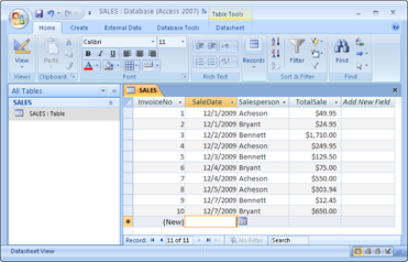
Figure 10-1: A result set for retrieval of sales from 12/01/2012 to 12/07/2012.

The result of this query, when run on Microsoft Access 2013 is shown in Figure 10-2. Running the query with a different database management system would retrieve the same result, but might appear a little different.

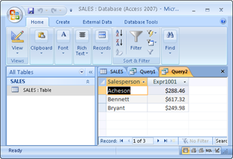
Figure 10-2: Average sales for each salesperson.

As shown in Figure 10-2, the average value of Bennett’s sales is considerably higher than that of the other two salespeople. You compare total sales with a similar query:

SELECT Salesperson, SUM(TotalSale)

   FROM SALES

   GROUP BY Salesperson;

This query gives the result shown in Figure 10-3.

Bennett also has the highest total sales, which is consistent with having the highest average sales.

Figure 10-3: Total sales for each salesperson.

HAVING Clauses

You can analyze the grouped data further by using the HAVING clause. The HAVING clause is a filter that acts similar to a WHERE clause, but on groups of rows rather than on individual rows. To illustrate the function of the HAVING clause, suppose the sales manager considers Bennett to be in a class by himself. His performance distorts the overall data for the other salespeople. (Aha — a curve-wrecker.) You can exclude Bennett's sales from the grouped data by using a HAVING clause as follows:

SELECT Salesperson, SUM(TotalSale)

   FROM SALES

   GROUP BY Salesperson

   HAVING Salesperson <>'Bennett';

This query gives you the result shown in Figure 10-4. Only rows where the salesperson is not Bennett are considered.

Figure 10-4: Total sales for all salespeople except Bennett.

ORDER BY Clauses

Use the ORDER BY clause to display the output table of a query in either ascending or descending alphabetical order. Whereas the GROUP BY clause gathers rows into groups and sorts the groups into alphabetical order, ORDER BY sorts individual rows. The ORDER BY clause must be the last clause that you specify in a query. If the query also contains a GROUP BY clause, the clause first arranges the output rows into groups. The ORDER BY clause then sorts the rows within each group. If you have no GROUP BY clause, then the statement considers the entire table as a group, and the ORDER BY clause sorts all its rows according to the column (or columns) that the ORDER BY clause specifies.

To illustrate this point, consider the data in the SALES table. The SALES table contains columns for InvoiceNo, SaleDate, Salesperson, and TotalSale. If you use the following example, you see all the data in the SALES table — but in an arbitrary order:

SELECT * FROM SALES ;

In one implementation, this may be the order in which you inserted the rows in the table; in another implementation, the order may be that of the most recent updates. The order can also change unexpectedly if anyone physically reorganizes the database. That's one reason it's usually a good idea to specify the order in which you want the rows. You may, for example, want to see the rows in order by the SaleDate like this:

SELECT * FROM SALES ORDER BY SaleDate ;

This example returns all the rows in the SALES table in order by SaleDate.

For rows with the same SaleDate, the default order depends on the implementation. You can, however, specify how to sort the rows that share the same SaleDate. You may want to see the sales for each SaleDate in order by InvoiceNo, as follows:

SELECT * FROM SALES ORDER BY SaleDate, InvoiceNo ;

This example first orders the sales by SaleDate; then for each SaleDate, it orders the sales by InvoiceNo. But don't confuse that example with the following query:

SELECT * FROM SALES ORDER BY InvoiceNo, SaleDate ;

This query first orders the sales by INVOICE_NO. Then for each different InvoiceNo, the query orders the sales by SaleDate. This probably won't yield the result you want, because it's unlikely that multiple sale dates will exist for a single invoice number.

The following query is another example of how SQL can return data:

SELECT * FROM SALES ORDER BY Salesperson, SaleDate ;

This example first orders by Salesperson and then by SaleDate. After you look at the data in that order, you may want to invert it, as follows:

SELECT * FROM SALES ORDER BY SaleDate, Salesperson ;

This example orders the rows first by SaleDate and then by Salesperson.

All these ordering examples are in ascending (ASC) order, which is the default sort order. The last SELECT shows earlier sales first — and, within a given date, shows sales for 'Adams' before 'Baker'. If you prefer descending (DESC) order, you can specify this order for one or more of the order columns, as follows:

SELECT * FROM SALES

ORDER BY SaleDate DESC, Salesperson ASC ;

This example specifies a descending order for sale dates, showing the more recent sales first, and an ascending order for salespeople, putting them in alphabetical order. That should give you a better picture of how Bennett’s performance stacks up against that of the other salespeople.

Limited FETCH

Whenever the ISO/IEC SQL standard is changed, it is usually to expand the capabilities of the language. This is a good thing. However, sometimes when you make such a change you cannot anticipate all the possible consequences. This happened with the addition of limited FETCH capability in SQL:2008.

The idea of the limited FETCH is that although a SELECT statement may return an indeterminate number of rows, perhaps you care only about the top three or perhaps the top ten. Pursuant to this idea, SQL:2008 added syntax shown in the following example:

SELECT Salesperson, AVG(TotalSale)

   FROM SALES

   GROUP BY Salesperson

   ORDER BY AVG(TotalSale) DESC

   FETCH FIRST 3 ROWS ONLY;

That looks fine. You want to see who your top three salespeople are in terms of those who are selling mostly high priced products. However, there is a small problem with this. What if three people are tied with the same average total sale, below the top two salespeople? Only one of those three will be returned. Which one? It is indeterminate.

Indeterminacy is intolerable to any self-respecting database person so this situation was corrected in SQL:2011. New syntax was added to include ties, in this manner:

SELECT Salesperson, AVG(TotalSale)

   FROM SALES

   GROUP BY Salesperson

   ORDER BY AVG(TotalSale) DESC

   FETCH FIRST 3 ROWS WITH TIES;

Now the result is completely determined: If there is a tie, you get all the tied rows. As before, if you leave off the WITH TIES modifier, the result is indeterminate.

A couple of additional enhancements were made to the limited FETCH capability in SQL:2011.

First, percentages are handled, as well as just a specific number of rows. Consider the following example:

SELECT Salesperson, AVG(TotalSale)

   FROM SALES

   GROUP BY Salesperson

   ORDER BY AVG(TotalSale) DESC

   FETCH FIRST 10 PERCENT ROWS ONLY;

It's conceivable that there might be a problem with ties when dealing with percentages, just as there is with a simple number of records, so the WITH TIES syntax may also be used here. You can include ties or not, depending on what you want in any particular situation.

Second, suppose you don’t want the top three or the top ten percent, but instead want the second three or second ten percent? Perhaps you want to skip directly to some point deep in the result set. SQL:2011 covers this situation also. The code would be similar to this:

SELECT Salesperson, AVG(TotalSale)

   FROM SALES

    GROUP BY Salesperson

   ORDER BY AVG(TotalSale) DESC

        OFFSET 3 ROWS

   FETCH NEXT 3 ROWS ONLY;

The OFFSET keyword tells how many rows to skip before fetching. The NEXT keyword specifies that the rows to be fetched are the ones immediately following the offset. Now the salespeople with the fourth, fifth, and sixth highest average sale total is returned. As you can see, without the WITH TIES syntax, there is still an indeterminacy problem. If the third, fourth, and fifth salespeople are tied, it is indeterminate which two will be included in this second batch and which one will have been included in the first batch.

It may be best to avoid using the limited FETCH capability. It’s too likely to deliver misleading results.

Peering through a Window to Create a Result Set

Windows and window functions were first introduced in SQL:1999. With a window, a user can optionally partition a data set, optionally order the rows in each partition, and specify a collection of rows (the window frame) that is associated with a given row.

The window frame of a row R is some subset of the partition containing R. For example, the window frame may consist of all the rows from the beginning of the partition up to and including R, based on the way rows are ordered in the partition.

A window function computes a value for a row R, based on the rows in the window frame of R.

For example, suppose you have a SALES table that has columns of CustID, InvoiceNo, and TotalSale. Your sales manager may want to know what the total sales were to each customer over a specified range of invoice numbers. You can obtain what she wants with the following SQL code:

SELECT CustID, InvoiceNo,

   SUM (TotalSale) OVER

   ( PARTITION BY CustID

     ORDER BY InvoiceNo

     ROWS BETWEEN

     UNBOUNDED PRECEDING

     AND CURRENT ROW )

   FROM SALES;

The OVER clause determines how the rows of the query are partitioned before being processed, in this case by the SUM function. A partition is assigned to each customer. Within each partition will be a list of invoice numbers, and associated with each of them will be the sum of all the TotalSale values over the specified range of rows, for each customer.

SQL:2011 has added several major enhancements to the original window functionality, incorporating new keywords.

Partitioning a window into buckets with NTILE

The NTILE window function apportions an ordered window partition into some positive integer number n of buckets, numbering the buckets from 1 to n. If the number of rows in a partition m is not evenly divisible by n, then after the NTILE function fills the buckets evenly, the remainder of m/n, called r, is apportioned to the first r buckets, making them larger than the other buckets.

Suppose you want to classify your employees by salary, partitioning them into five buckets, from highest to lowest. You can do it with the following code:

SELECT FirstName, LastName, NTILE (5)

   OVER (ORDER BY Salary DESC)

   AS BUCKET

   FROM Employee;

If there are, for example, 11 employees, each bucket is filled with two except for the first bucket, which is filled with three. The first bucket will contain the three highest paid employees, and the fifth bucket will contain the two lowest paid employees.

Navigating within a window

Added in SQL:2011 are five window functions that evaluate an expression in a row R2 that is somewhere in the window frame of the current row R1. The functions are LAG, LEAD, NTH_VALUE, FIRST_VALUE, and LAST_VALUE.

These functions enable you to pull information from specified rows that are within the window frame of the current row.

Looking back with the LAG function

The LAG function enables you to retrieve information from the current row in the window you're examining as well as information from another row that you specify that precedes the current row.

Suppose, for example, that you have a table that records the total sales for each day for the current year. One thing you might want to know is how today's sales compare to yesterday's. You could do this with the LAG function, as follows:

SELECT TotalSale AS TodaySale,

   LAG (TotalSale) OVER

   (ORDER BY SaleDate) AS PrevDaySale

   FROM DailyTotals;

For each row in DailyTotals, this query would return a row listing that row's total sales figure and the previous day's total sales figure. The default offset is 1, which is why the previous day's result is returned rather than any other.

To compare the current day’s sales to those of a week prior, you could use the following:

SELECT TotalSale AS TodaySale,

   LAG (TotalSale, 7) OVER

   (ORDER BY SaleDate) AS PrevDaySale

   FROM DailyTotals;

The first seven rows in a window frame will not have a predecessor that is a week older. The default response to this situation is to return a null result for PrevDaySale. If you would prefer some other result to a null result, for example zero, you can specify what you want returned in this situation instead of the default null value, for example, 0 (zero), as shown here:

SELECT TotalSale AS TodaySale,

   LAG (TotalSale, 7, 0) OVER

   (ORDER BY SaleDate) AS PrevDaySale

   FROM DailyTotals;

The default behavior is to count rows that have a lag extent, which in this case is TotalSale, which contains a null value. If you want to skip over such rows and count only rows that have an actual value in the lag extent, you can do so by adding the keywords IGNORE NULLS as shown in the following variant of the example:

SELECT TotalSale AS TodaySale,

   LAG (TotalSale, 7, 0) IGNORE NULLS

   OVER (ORDER BY SaleDate) AS PrevDaySale

   FROM DailyTotals;

Looking ahead with the LEAD function

The LEAD window function operates exactly the same way the LAG function operates except that, instead of looking back to a preceding row, it looks ahead to a row following the current row in the window frame. An example might be:

SELECT TotalSale AS TodaySale,

   LEAD (TotalSale, 7, 0) IGNORE NULLS

   OVER (ORDER BY SaleDate) AS NextDaySale

   FROM DailyTotals;

Looking to a specified row with the NTH_VALUE function

The NTH_VALUE function is similar to the LAG and LEAD functions, except that instead of evaluating an expression in a row preceding or following the current row, it evaluates an expression in a row that is at a specified offset from the first or the last row in the window frame.

Here’s an example:

SELECT TotalSale AS ChosenSale,

   NTH_VALUE (TotalSale, 2)

   FROM FIRST

   IGNORE NULLS

   OVER (ORDER BY SaleDate)

   ROWS BETWEEN 10 PRECEDING AND 10 FOLLOWING )

        AS EarlierSale

   FROM DailyTotals;

In this example, EarlierSale is evaluated as follows:

The window frame associated with the current row is formed. It includes the ten preceding and the ten following rows.

TotalSale is evaluated in each row of the window frame.

IGNORE NULLS is specified, so any rows containing a null value for TotalSale are skipped.

Starting from the first value remaining after the exclusion of rows containing a null value for TotalSale, move forward by two rows (forward because FROM FIRST was specified).

The value of EarlierSale is the value of TotalSale from the specified row.

If you don't want to skip rows that have a null value for TotalSale, specify RESPECT NULLS rather than IGNORE NULLS. The NTH_VALUE function works similarly if you specify FROM LAST instead of FROM FIRST, except instead of counting forward from the first record in the window frame, you count backward from the last record in the window frame. The number specifying the number of rows to count is still positive, even though you're counting backward rather than forward.

Looking to a very specific value with FIRST_VALUE and LAST_VALUE

The FIRST_VALUE and LAST_VALUE functions are special cases of the NTH_VALUE function. FIRST_VALUE is equivalent to NTH_VALUE where FROM FIRST is specified and the offset is 0 (zero). LAST_VALUE is equivalent to NTH_VALUE where FROM LAST is specified and the offset is 0. With both of these, you can choose to either ignore or respect nulls.

Nesting window functions

Sometimes to get the result you need, the easiest way is to nest one function within another. SQL:2011 added the capability to do such nesting with window functions.

As an example, consider a case where a stock investor is trying to determine whether it is a good time to buy a particular stock. To get a handle on this, she decides to compare the current stock price to the price it sold for on the immediately previous 100 trades. She wonders, how many times in the previous 100 trades it sold for less than the current price. To reach an answer, she makes the following query:

SELECT SaleTime,

   SUM ( CASE WHEN SalePrice <

   VALUE OF (SalePrice AT CURRENT ROW)

   THEN 1 ELSE 0 )

   OVER (ORDER BY SaleTime

   ROWS BETWEEN 100 PRECEDING AND CURRENT ROW )

  FROM StockSales;

The window encompasses the 100 rows preceding the current row, which correspond to the 100 sales immediately prior to the current moment. Every time a row is evaluated where the value of SalePrice is less than the most recent price, 1 is added to the sum. The end result is a number that tells you the number of sales out of the previous hundred that were made at a lower price than the current price.

Evaluating groups of rows

Sometimes the sort key you have chosen to place a partition in order will have duplicates. You may want to evaluate all rows that have the same sort key as a group. In such cases you can use the GROUPS option. With it you can count groups of rows where the sort keys are identical.

Here’s an example:

SELECT CustomerID, SaleDate,

   SUM (InvoiceTotal) OVER

   ( PARTITION BY CustomerID

     ORDER BY SaleDate

   GROUPS BETWEEN 2 PRECEDING AND 2 FOLLOWING )

  FROM Customers;

The window frame in this example consists of up to five groups of rows: two groups before the group containing the current row, the group containing the current row, and two groups following the group containing the current row. The rows in each group have the same SaleDate, and the SaleDate associated with each group is different from the SaleDate values for the other groups.