Chapter 2
![]()
In the first chapter, I stressed the importance of having a performance baseline that you can use to measure performance changes. In fact, this is one of the first things you should do when starting the performance tuning process, since without a baseline you will not be able to quantify improvements. In this chapter, you will learn how to use the Performance Monitor tool to accomplish this and how to use the different performance counters that are required to create a baseline. Other tools necessary for establishing baseline performance metrics for the system will also be addressed when they can help you above and beyond what the Performance Monitor tool can do.
Specifically, I cover the following topics:
- The basics of the Performance Monitor tool
- How to analyze hardware resource bottlenecks using Performance Monitor
- How to retrieve Performance Monitor data within SQL Server using dynamic management views
- How to resolve hardware resource bottlenecks
- How to analyze the overall performance of SQL Server
- Considerations for monitoring virtual machines
- How to create a baseline for the system
Performance Monitor Tool
Windows Server 2008 provides a tool called Performance Monitor. Performance Monitor collects detailed information about the utilization of operating system resources. It allows you to track nearly every aspect of system performance, including memory, disk, processor, and the network. In addition, SQL Server 2012 provides extensions to the Performance Monitor tool to track a variety of functional areas within SQL Server.
Performance Monitor tracks resource behavior by capturing performance data generated by hardware and software components of the system, such as a processor, a process, a thread, and so on. The performance data generated by a system component is represented by a performance object. A performance object provides counters that represent specific aspects of a component, such as % Processor Time for a Processor object. Just remember, when running these counters within a virtual machine (VM), the performance measured for the counters in most instances is for the VM, not the physical server.
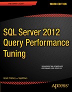
There can be multiple instances of a system component. For instance, the Processor object in a computer with two processors will have two instances represented as instances 0 and 1. Performance objects with multiple instances may also have an instance called Total to represent the total value for all the instances. For example, the processor usage of a computer with four processors can be determined using the following performance object, counter, and instance (as shown in Figure 2-1):
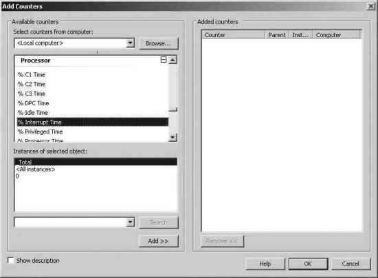
Figure 2-1. Adding a Performance Monitor counter
- Performance object: Processor
- Counter: % Processor Time
- Instance: _Total
System behavior can be either tracked in real time in the form of graphs or captured as a log (called a data collector set) for offline analysis. The preferred mechanism on production servers is to use the log.
To run the Performance Monitor tool, execute perfmon from a command prompt, which will open the Performance Monitor suite. You can also right-click the Computer icon on the desktop or the Start menu, expand Diagnostics, and then expand the Performance Monitor. Both will allow you to open the Performance Monitor utility.
You will learn how to set up the individual counters in the “Creating a Baseline” section later in this chapter. First, let’s examine which counters you should choose in order to identify system bottlenecks and how to resolve some of these bottlenecks.
To get an immediate snapshot of a large amount of data that was formerly available only in Performance Monitor, SQL Server now offers the same data internally through a set of dynamic management views (DMVs) and dynamic management functions (DMFs) collectively referred to as dynamic management objects (DMOs). These are extremely useful mechanisms for capturing a snapshot of the current performance of your system. I’ll introduce several throughout the book, but for now I’ll focus on a few that are the most important for monitoring performance and for establishing a baseline.
The sys.dm_os_performance_counters view displays the SQL Server counters within a query, allowing you to apply the full strength of T-SQL to the data immediately. For example, this simple query will return the current value for Logins/sec:
SELECT dopc.cntr_value,
dopc.cntr_type
FROM sys.dm_os_performance_counters AS dopc
WHERE dopc.object_name = 'MSSQL$RANDORI:General Statistics'
AND dopc.counter_name = 'Logins/sec';
This returns the value of 15 for my server. For your server, you’ll need to substitute the appropriate server name in the object_name comparison. Worth noting is the cntr_type column. This column tells you what type of counter you’re reading (documented by Microsoft at http://msdn.microsoft.com/en-us/library/aa394569(VS.85).aspx). For example, the counter above returns the value 272696576, which means that this counter is an average value. There are values that are moments-in-time snapshots, accumulations since the server started, and others. Knowing what the measure represents is an important part of understanding these metrics.
There are a large number of DMOs that can be used to gather information about the server. I’ll be covering many of these throughout the book. I’ll introduce one more here that you will find yourself accessing on a regular basis, sys.dm_os_wait_stats. This DMV shows an aggregated view of the threads within SQL Server that are waiting on various resources, collected since the last time SQL Server was started or the counters were reset. Identifying the types of waits that are occurring within your system is one of the easiest mechanisms to begin identifying the source of your bottlenecks. You can sort the data in various ways; this first example looks at the waits that have the longest current count using this simple query:
SELECT TOP (10) dows.*
FROM sys.dm_os_wait_stats AS dows
ORDER BY dows.wait_time_ms DESC;
Figure 2-2 displays the output.
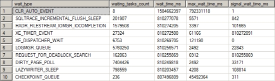
Figure 2-2. Output from sys.dm_os_wait_stats
You can see not only the cumulative time that particular waits have accumulated but also a count of how often they have occurred and the maximum time that something had to wait. From here, you can identify the wait type and begin troubleshooting. One of the most common types of waits is I/O. If you see ASYNCH_I0_C0MPLETI0N, I0_C0MPLETI0N, LOGMGR, WRITELOG, or PAGEIOLATCH in your top ten wait types, you may be experiencing I/O contention, and you now know where to start working. For a more detailed analysis of wait types and how to use them as a monitoring tool within SQL Server, read the Microsoft white paper “SQL Server 2005 Waits and Queues” ( http://download.microsoft.com/download/4/7/a/47a548b9-249e-484c-abd7-29f31282b04d/Performance_Tuning_Waits_Queues.doc). Although it was written for SQL Server 2005, it is still largely applicable to newer versions of SQL Server. You can always find information about more obscure wait types by going directly to Microsoft at support.microsoft.com. Finally, when it comes to wait types, Bob Ward’s repository (collected at http://blogs.msdn.com/b/psssql/archive/2009/11/03/the-sql-server-wait-type-repository.aspx) is a must read.
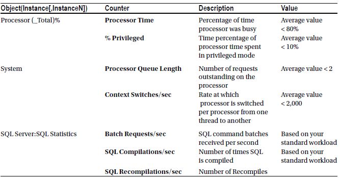
Typically, SQL Server database performance is affected by stress on the following hardware resources:
- Memory
- Disk I/O
- Processor
- Network
Stress beyond the capacity of a hardware resource forms a bottleneck. To address the overall performance of a system, you need to identify these bottlenecks because they form the limit on overall system performance.
There is usually a relationship between resource bottlenecks. For example, a processor bottleneck may be a symptom of excessive paging (memory bottleneck) or a slow disk (disk bottleneck). If a system is low on memory, causing excessive paging, and has a slow disk, then one of the end results will be a processor with high utilization since the processor has to spend a significant number of CPU cycles to swap pages in and out of the memory and to manage the resultant high number of I/O requests. Replacing the processors with faster ones may help a little, but it is not be the best overall solution. In a case like this, increasing memory is a more appropriate solution because it will decrease pressure on the disk and processor as well. In fact, upgrading the disk is probably a better solution than upgrading the processor.
![]() Note The most common performance problem is usually I/O, either from memory or from the disk.
Note The most common performance problem is usually I/O, either from memory or from the disk.
One of the best ways of locating a bottleneck is to identify resources that are waiting for some other resource to complete its operation. You can use Performance Monitor counters or DMOs such as sys.dm_os_wait_stats to gather that information. The response time of a request served by a resource includes the time the request had to wait in the resource queue as well as the time taken to execute the request, so end user response time is directly proportional to the amount of queuing in a system.
Another way to identify a bottleneck is to reference the response time and capacity of the system. The amount of throughput, for example, to your disks should normally be something approaching what the vendor suggests that the disk is capable of. So measuring information from your performance monitor such as disk sec/transfer will give you an indication of when disks are slowing down due to excessive load.
Not all resources have specific counters that show queuing levels, but most resources have some counters that represent an overcommittal of that resource. For example, memory has no such counter, but a large number of hard page faults represents the overcommittal of physical memory (hard page faults are explained later in the chapter in the section “Pages/sec and Page Faults/sec Counters”). Other resources, such as the processor and disk, have specific counters to indicate the level of queuing. For example, the counter Page Life Expectancy indicates how long a page will stay in the buffer pool without being referenced. This is an indicator of how well SQL Server is able to manage its memory, since a longer life means that a piece of data in the buffer will be there, available, waiting for the next reference. However, a shorter life means that SQL Server is moving pages in and out of the buffer quickly, possibly suggesting a memory bottleneck.
You will see which counters to use in analyzing each type of bottleneck shortly.
Once you have identified bottlenecks, you can resolve them in two ways.
- You can increase resource capacity.
- You can decrease the arrival rate of requests to the resource.
Increasing the throughput usually requires extra resources such as memory, disks, processors, or network adapters. You can decrease the arrival rate by being more selective about the requests to a resource. For example, when you have a disk subsystem bottleneck, you can either increase the capacity of the disk subsystem or decrease the amount of I/O requests.
Increasing the capacity means adding more disks or upgrading to faster disks. Decreasing the arrival rate means identifying the cause of high I/O requests to the disk subsystem and applying resolutions to decrease their number. You may be able to decrease the I/O requests, for example, by adding appropriate indexes on a table to limit the amount of data accessed or by partitioning a table between multiple disks.
Memory can be a problematic bottleneck because a bottleneck in memory will manifest on other resources, too. This is particularly true for a system running SQL Server. When SQL Server runs out of cache (or memory), a process within SQL Server (called lazy writer) has to work extensively to maintain enough free internal memory pages within SQL Server. This consumes extra CPU cycles and performs additional physical disk I/O to write memory pages back to disk.
The good news is that SQL Server 2012 has changed memory management. A single process now manages all memory within SQL Server; this can help to avoid some of the bottlenecks previously encountered because max server memory will be applied to all processes, not just those smaller than 8k in size.
SQL Server manages memory for databases, including memory requirements for data and query execution plans, in a large pool of memory called the buffer pool. The memory pool used to consist of a collection of 8KB buffers to manage memory. Now there are multiple page allocations for data pages and plan cache pages, free pages, and so forth. The buffer pool is usually the largest portion of SQL Server memory. SQL Server manages memory by growing or shrinking its memory pool size dynamically.
You can configure SQL Server for dynamic memory management in SQL Server Management Studio (SSMS). Go to the Memory folder of the Server Properties dialog box, as shown in Figure 2-3.
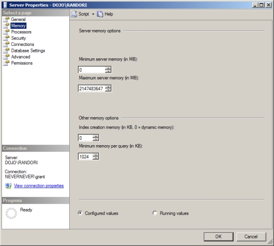
Figure 2-3. SQL Server memory configuration
The dynamic memory range is controlled through two configuration properties: Minimum(MB) and Maximum(MB).
- Minimum(MB), also known as min server memory, works as a floor value for the memory pool. Once the memory pool reaches the same size as the floor value, SQL Server can continue committing pages in the memory pool, but it can’t be shrunk to less than the floor value. Note that SQL Server does not start with the min server memory configuration value but commits memory dynamically, as needed.
- Maximum(MB), also known as max server memory, serves as a ceiling value to limit the maximum growth of the memory pool. These configuration settings take effect immediately and do not require a restart. In SQL Server 2012 the lowest maximum memory is now 64MB for a 32-bit system and 128MB for a 64-bit system.
Microsoft recommends that you use dynamic memory configuration for SQL Server, where min server memory is 0 and max server memory is set to allow some memory for the operating system, assuming a single instance on the machine. The amount of memory for the operating system depends on the system itself. For most systems with 8-16GB of memory, you should leave about 2GB for the OS. You’ll need to adjust this depending on your own system’s needs and memory allocations. You should not run other memory-intensive applications on the same server as SQL Server, but if you must, I recommend you first get estimates on how much memory is needed by other applications and then configure SQL Server with a max server memory value set to prevent the other applications from starving SQL Server of memory. On a system where SQL Server is running on its own, I prefer to set the minimum server memory equal to the max value and simply dispatch with dynamic management. On a server with multiple SQL Server instances, you’ll need to adjust these memory settings to ensure each instance has an adequate value. Just make sure you’ve left enough memory for the operating system and external processes.
Memory within SQL Server can be roughly divided into buffer pool memory, which represents data pages and free pages, and nonbuffer memory, which consists of threads, DLLs, linked servers, and others. Most of the memory used by SQL Server goes into the buffer pool. But you can get allocations beyond the buffer pool, known as private bytes, which can cause memory pressure not evident in the normal process of monitoring the buffer pool. Check Process: sqlservr: Private Bytes in comparison to SQL Server: Buffer Manager: Total pages if you suspect this issue on your system.
You can also manage the configuration values for min server memory and max server memory by using the sp_configure system stored procedure. To see the configuration values for these parameters, execute the sp_configure stored procedure as follows:
EXEC sp_configure 'show advanced options', 1;
GO
RECONFIGURE;
GO
EXEC sp_configure 'min server memory';
EXEC sp_configure 'max server memory';
Figure 2-4 shows the result of running these commands.
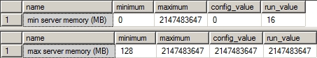
Figure 2-4. SQL Server memory configuration properties
Note that the default value for the min server memory setting is 0MB and for the max server memory setting is 2147483647MB. Also, max server memory can’t be set to less than 64MB on a 32-bit machine and 128MB on a 64-bit machine.
You can also modify these configuration values using the spconfigure stored procedure. For example, to set max server memory to 200MB and min server memory to 100MB, execute the following set of statements (setmemory.sql in the download):
USE master;
EXEC sp_configure 'show advanced option', 1;
RECONFIGURE;
exec sp_configure 'min server memory (MB)', 128;
exec sp_configure 'max server memory (MB)', 200;
RECONFIGURE WITH OVERRIDE;
The min server memory and max server memory configurations are classified as advanced options. By default, the sp_configure stored procedure does not affect/display the advanced options. Setting show advanced option to 1 as shown previously enables the sp_configure stored procedure to affect/display the advanced options.
The RECONFIGURE statement updates the memory configuration values set by sp_configure. Since ad hoc updates to the system catalog containing the memory configuration values are not recommended, the OVERRIDE flag is used with the RECONFIGURE statement to force the memory configuration. If you do the memory configuration through Management Studio, Management Studio automatically executes the RECONFIGURE WITH OVERRIDE statement after the configuration setting.
You may need to allow for SQL Server sharing a system’s memory. To elaborate, consider a computer with SQL Server and SharePoint running on it. Both servers are heavy users of memory and thus keep pushing each other for memory. The dynamic memory behavior of SQL Server allows it to release memory to SharePoint at one instance and grab it back as SharePoint releases it. You can avoid this dynamic memory management overhead by configuring SQL Server for a fixed memory size. However, please keep in mind that since SQL Server is an extremely resource-intensive process, it is highly recommended that you have a dedicated SQL Server production machine.
Now that you understand SQL Server memory management at a very high level, let’s consider the performance counters you can use to analyze stress on memory, as shown in Table 2-1.
Table 2-1. Performance Monitor Counters to Analyze Memory Pressure
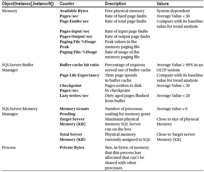
I’ll now walk you through these counters to get a better idea of possible uses.
Available Bytes
The Available Bytes counter represents free physical memory in the system. You can also look at Available Kbytes and Available Mbytes for the same data but with less granularity. For good performance, this counter value should not be too low. If SQL Server is configured for dynamic memory usage, then this value will be controlled by calls to a Windows API that determines when and how much memory to release. Extended periods of time with this value very low and SQL Server memory not changing indicates that the server is under severe memory stress.
Pages/sec and Page Faults/sec
To understand the importance of the Pages/sec and Page Faults/sec counters, you first need to learn about page faults. A page fault occurs when a process requires code or data that is not in its working set (its space in physical memory). It may lead to a soft page fault or a hard page fault. If the faulted page is found elsewhere in physical memory, then it is called a soft page fault. A hard page fault occurs when a process requires code or data that is not in its working set or elsewhere in physical memory and must be retrieved from disk.
The speed of a disk access is in the order of milliseconds, whereas a memory access is in the order of nanoseconds. This huge difference in the speed between a disk access and a memory access makes the effect of hard page faults significant compared to that of soft page faults.
The Pages/sec counter represents the number of pages read from or written to disk per second to resolve hard page faults. The Page Faults/sec performance counter indicates the total page faults per second—soft page faults plus hard page faults—handled by the system. These are primarily measures of load and are not direct indicators of performance issues.
Hard page faults, indicated by Pages/sec, should not be consistently higher than normal. There are no hard and fast numbers for what indicates a problem because these numbers will vary widely between systems based on the amount and type of memory as well as the speed of disk access on the system.
If the Pages/sec counter is very high, you can break it up into Pages Input/sec and Pages Output/sec.
- Pages Input/sec: An application will wait only on an input page, not on an output page.
- Pages Output/sec: Page output will stress the system, but an application usually does not see this stress. Pages output are usually represented by the application’s dirty pages that need to be backed out to the disk. Pages Output/sec is an issue only when disk load become an issue.
Also, check Process:Page Faults/sec to find out which process is causing excessive paging in case of high Pages/sec. The Process object is the system component that provides performance data for the processes running on the system, which are individually represented by their corresponding instance name.
For example, the SQL Server process is represented by the sqlservr instance of the Process object. High numbers for this counter usually do not mean much unless Pages/sec is high. Page Faults/sec can range all over the spectrum with normal application behavior, with values from 0 to 1,000 per second being acceptable. This entire data set means a baseline is essential to determine the expected normal behavior.
Paging File %Usage and Page File %Usage
All memory in the Windows system is not the physical memory of the physical machine. Windows will swap memory that isn’t immediately active in and out of the physical memory space to a paging file. These counters are used to understand how often this is occurring on your system. As a general measure of system performance, these counters are only applicable to the Windows OS and not to SQL Server. However, the impact of not enough virtual memory will affect SQL Server. These counters are collected in order to understand whether the memory pressures on SQL Server are internal or external. If they are external memory pressures, you will need to go into the Windows OS to determine what the problems might be.
The buffer cache is the pool of buffer pages into which data pages are read, and it is often the biggest part of the SQL Server memory pool. This counter value should be as high as possible, especially for OLTP systems that should have fairly regimented data access, unlike a warehouse or reporting system. It is extremely common to find this counter value as 99 percent or more for most production servers. A low Buffer cache hit ratio value indicates that few requests could be served out of the buffer cache, with the rest of the requests being served from disk.
When this happens, either SQL Server is still warming up or the memory requirement of the buffer cache is more than the maximum memory available for its growth. If the cache hit ratio is consistently low, you should consider getting more memory for the system or reducing memory requirements through the use of good indexes and other query tuning mechanism. That is, unless you’re dealing with a reporting systems with lots of ad hoc queries. It’s possible with reporting systems to consistently see the cache hit ratio become extremely low.
Page Life Expectancy indicates how long a page will stay in the buffer pool without being referenced. Generally, a low number for this counter means that pages are being removed from the buffer, lowering the efficiency of the cache and indicating the possibility of memory pressure. On reporting systems, as opposed to OLTP systems, this number may remain at a lower value since more data is accessed from reporting systems. Since this is very dependent on the amount of memory you have available and the types of queries running on your system, there are no hard and fast numbers that will satisfy a wide audience. Therefore, you will need to establish a baseline for your system and monitor it over time.
Checkpoint Pages/sec
The Checkpoint Pages/sec counter represents the number of pages that are moved to disk by a checkpoint operation. These numbers should be relatively low, for example, less than 30 per second for most systems. A higher number means more pages are being marked as dirty in the cache. A dirty page is one that is modified while in the buffer. When it’s modified, it’s marked as dirty and will get written back to the disk during the next checkpoint. Higher values on this counter indicate a larger number of writes occurring within the system, possibly indicative of I/O problems. But, if you are taking advantage of the new indirect checkpoints, which allow you to control when checkpoints occur in order to reduce recovery intervals, you might see different numbers here. Take that into account when monitoring databases with the indirect checkpoint configured.
Lazy writes/sec
The Lazy writes/sec counter records the number of buffers written each second by the buffer manager’s lazy write process. This process is where the dirty, aged buffers are removed from the buffer by a system process that frees the memory up for other uses. A dirty, aged buffer is one that has changes and needs to be written to the disk. Higher values on this counter possibly indicate I/O issues or even memory problems. The Lazy writes/sec values should consistently be less than 20 for the average system.
Memory Grants Pending
The Memory Grants Pending counter represents the number of processes pending for a memory grant within SQL Server memory. If this counter value is high, then SQL Server is short of memory. Under normal conditions, this counter value should consistently be 0 for most production servers.
Another way to retrieve this value, on the fly, is to run queries against the DMV sys.dm_ exec_query_memory_grants. A null value in the column grant_time indicates that the process is still waiting for a memory grant. This is one method you can use to troubleshoot query timeouts by identifying that a query (or queries) is waiting on memory in order to execute.
Target Server Memory (KB) and Total Server Memory (KB)
Target Server Memory (KB) indicates the total amount of dynamic memory SQL Server is willing to consume. Total Server Memory (KB) indicates the amount of memory currently assigned to SQL Server. The Total Server Memory (KB) counter value can be very high if the system is dedicated to SQL Server. If Total Server Memory (KB) is much less than Target Server Memory (KB), then either the SQL Server memory requirement is low, the max server memory configuration parameter of SQL Server is set at too low a value, or the system is in warm-up phase. The warm-up phase is the period after SQL Server is started when the database server is in the process of expanding its memory allocation dynamically as more data sets are accessed, bringing more data pages into memory.
You can confirm a low memory requirement from SQL Server by the presence of a large number of free pages, usually 5,000 or more. Also you can directly check the status of memory by querying the DMO sys.dm_os_ring_buffers, which returns information about memory allocation within SQL Server.
Additional Memory Monitoring Tools
While you can get the basis for the behavior of memory within SQL Server from the Performance Monitor counters, once you know that you need to spend time looking at your memory usage, you’ll need to take advantage of other tools and tools sets. The following are some of the commonly used reference points for identifying memory issues on a SQL Server system. Some of these tools, while actively used by large numbers of the SQL Server community, are not documented within SQL Server Books Online. This means they are absolutely subject to change or removal.
This command goes into the SQL Server memory and reads out the current allocations. It’s a moment-in-time measurement, a snapshot. It gives you a set of measures of where memory is currently allocated. The results from running the command come back as two basic result sets, as you can see in Figure 2-5.
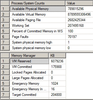
Figure 2-5. Output of DBCC MEMORYSTATUS
The first data set shows basic allocations of memory and counts of occurrences. For example, the Available Physical Memory is a measure of the memory available on the system where as the Page Faults is just a count of the number of page faults that have occurred.
The second data set shows different memory managers within SQL Server and the amount of memory that they have consumed at the moment that the MEMORYSTATUS command was called.
Each of these can be used to understand where memory allocation is occurring within the system. For example, in most systems, most of the time the primary consumer of memory is the buffer cache. You can compare the Target Committed value to the Current Committed value to understand if you’re seeing pressure on the buffer cache. When the Target is higher than the Current, you might be seeing buffer cache problems and need to figure out which process within your currently executing SQL Server processes is using the most memory. This can be done using a Dynamic Management Object.
Dynamic Management Objects
There are a large number of memory-related DMOs within SQL Server. Several of them have been updated with SQL Server 2012. Reviewing all of them is outside the scope of this book. The following four are the most frequently used when determining if you have memory bottlenecks within SQL Server.
While most of the memory within SQL Server is allocated to the buffer cache, there are a number of processes within SQL Server that also can, and will, consume memory. These processes expose their memory allocations through this DMO. You can use this to see what processes might be taking resources away from the buffer cache in the event you have other indications of a memory bottleneck.
A memory clerk is the process that allocates memory within SQL Server. Looking at what these processes are up to allows you to understand if there are internal memory allocation issues going on within SQL Server that might rob the procedure cache of needed memory. If the Performance Monitor counter for Private Bytes is high, you can determine which parts of the system are being consumed through the DMV.
This DMV is not documented within the Books Online, so it is subject to change or removal. This DMV outputs as XML. You can usually read the output by eye, but you may need to implement XQuery to get really sophisticated reads from the ring buffers.
A ring buffer is nothing more than a recorded response to a notification. These are kept within this DMV and accessing it allows you to see things changing within your memory. The main ring buffers associated with memory are listed in Table 2-2.
Table 2-2 . Main Ring Buffers Associated with Memory
| Ring Buffer | Ring_buffer_type | Use |
| Resource Monitor | RING_BUFFER_ RESOURCE_MONITOR |
As memory allocation changes, notifications of this change are recorded here. This information can be very useful for identifying external memory pressure. |
| Out Of Memory | RING_BUFFER_OOM | When you get out-of-memory issues, they are recorded here so you can tell what kind of memory action failed. |
| Memory Broker | RING_BUFFER_ MEMORY_BROKER |
As the memory internal to SQL Server drops, a low memory notification will force processes to release memory for the buffer. These notifications are recorded here, making this a useful measure for when internal memory pressure occurs. |
| Buffer Pool | RING_BUFFER_ BUFFER_POOL |
Notifications of when the buffer pool itself is running out of memory are recorded here. This is just a general indication of memory pressure. |
There are other ring buffers available, but they are not applicable to memory allocation issues.
When there is high stress on memory, indicated by a large number of hard page faults, you can resolve memory bottleneck using the flowchart shown in Figure 2-6.
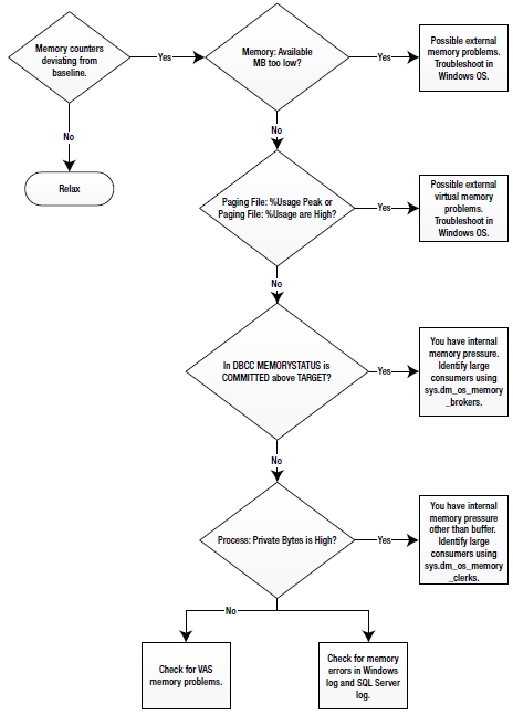
Figure 2-6. Memory bottleneck resolution chart
A few of the common resolutions for memory bottlenecks are as follows:
- Optimizing application workload
- Allocating more memory to SQL Server
- Increasing system memory
- Changing from a 32-bit to a 64-bit processor
- Enabling 3GB of process space
- Data Compression
Let’s take a look at each of these in turn.
Optimizing Application Workload
Optimizing application workload is the most effective resolution most of the time, but because of the complexity and challenges involved in this process, it is usually considered last. To identify the memory-intensive queries, capture all the SQL queries using Extended Events (which you will learn how to use in Chapter 3), and then group the trace output on the Reads column. The queries with the highest number of logical reads contribute most often to memory stress, but there is not a linear correlation between the two. You will see how to optimize those queries in more detail throughout this book.
Allocating More Memory to SQL Server
As you learned in the “SQL Server Memory Management” section, the max server memory configuration can limit the maximum size of the SQL Server memory pool. If the memory requirement of SQL Server is more than the max server memory value, which you can tell through the number of hard page faults, then increasing the value will allow the memory pool to grow. To benefit from increasing the max server memory value, ensure that enough physical memory is available in the system.
Increasing System Memory
The memory requirement of SQL Server depends on the total amount of data processed by SQL activities. It is not directly correlated to the size of the database or the number of incoming SQL queries. For example, if a memory-intensive query performs a cross join between two small tables without any filter criteria to narrow down the result set, it can cause high stress on the system memory.
One of the easiest and quickest resolutions is to simply increase system memory by purchasing and installing more. However, it is still important to find out what is consuming the physical memory because if the application workload is extremely memory intensive, you will soon be limited by the maximum amount of memory a system can access. To identify which queries are using more memory, query the sys.dm_exec_query_memory_grants DMV. Just be careful when running queries against this DMV using a JOIN or an ORDER BY statement; if your system is already under memory stress, these actions can lead to your query needing its own memory grant.
Changing from a 32-bit to a 64-bit Processor
Switching the physical server from a 32-bit processor to a 64-bit processor (and the attendant Windows Server software upgrade) radically changes the memory management capabilities of SQL Server. The limitations on SQL Server for memory go from 3GB to a limit of up to 8TB depending on the version of the operating system and the specific processor type.
Prior to SQL Server 2012, it was possible to add up to 64GB of data cache to a SQL Server instance through the use of Address Windowing Extensions. These have now been removed from SQL Server 2012, so a 32-bit instance of SQL Server is limited to accessing only 3GB of memory. Only very small systems should be running 32-bit versions of SQL Server 2012 because of this limitation.
Data compression has a number of excellent benefits for storage and retrieval of information. It has an added benefit that many people aren’t aware of: while compressed information is stored in memory, it remains compressed. This means more information can be moved while using less system memory, increasing your overall memory throughput. All this does come at some cost to the CPU, so you’ll need to keep an eye on that to be sure you’re not just transferring stress.
Enabling 3GB of Process Address Space
Standard 32-bit addresses can map a maximum of 4GB of memory. The standard address spaces of 32-bit Windows operating systems processes are therefore limited to 4GB. Out of this 4GB process space, by default the upper 2GB is reserved for the operating system, and the lower 2GB is made available to the application. If you specify a /3GB switch in the boot.ini file of the 32-bit OS, the operating system reserves only 1GB of the address space and the application can access up to 3GB. This is also called 4-gig tuning (4GT). No new APIs are required for this purpose.
Therefore, on a machine with 4GB of physical memory and the default Windows configuration, you will find available memory of about 2GB or more. To let SQL Server use up to 3GB of the available memory, you can add the /3GB switch in the boot.ini file as follows:
[boot loader]
timeout=30
default=multi(o)disk(o)rdisk(o)partition(l)WINNT
[operating systems]
multi(o)disk(o)rdisk(o)partition(l)WINNT=
"Microsoft Windows Server 2008 Advanced Server"
/fastdetect /3GB
The /3GB switch should not be used for systems with more than 16GB of physical memory, as explained in the following section, or for systems that require a higher amount of kernel memory.
SQL Server 2012 on 64-bit systems can support up to 8TB on an x64 platform As more memory is available from the OS, the limits imposed by SQL Server are reached. This is without having to use any other switches or extended memory schemes.
SQL Server can have demanding I/O requirements, and since disk speeds are comparatively much slower than memory and processor speeds, a contention in disk resources can significantly degrade SQL Server performance. Analysis and resolution of any disk resource bottleneck can improve SQL Server performance significantly.
To analyze disk performance, you can use the counters shown in Table 2-3.
Table 2-3. Performance Monitor Counters to Analyze I/O Pressure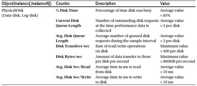
The PhysicalDisk counters represent the activities on a physical disk. LogicalDisk counters represent logical subunits (or partitions) created on a physical disk. If you create two partitions, say R: and S: on a physical disk, then you can monitor the disk activities of the individual logical disks using logical disk counters. However, because a disk bottleneck ultimately occurs on the physical disk, not on the logical disk, it is usually preferable to use the PhysicalDisk counters.
Note that for a hardware redundant array of independent disks (RAID) subsystem (see the “Using a RAID Array” section for more on RAID), the counters treat the array as a single physical disk. For example, even if you have ten disks in a RAID configuration, they will all be represented as one physical disk to the operating system, and subsequently you will have only one set of PhysicalDisk counters for that RAID subsystem. The same point applies to storage area network (SAN) disks (see the “Using a SAN System” section for specifics). Because of this, some of the numbers represented in the previous tables may be radically lower (or higher) than what your system can support.
Take all these numbers as general guidelines for monitoring your disks and adjust the numbers to take into account the fact that technology is constantly shifting and you may see very different performance as the hardware improves. We’re moving into more and more solid state drives (SSD) and even SSD arrays that make disk I/O operator orders of magnitude faster. Where we’re not moving in SSD, we’re taking advantage of iSCSI interfaces. As you introduce or work with these types of hardware, keep in mind that these numbers are more in line with platter style disk drives.
% Disk Time
The % Disk Time counter monitors the percentage of time the disk is busy with read/write activities. This is a good indicator of load, but not a specific indicator of issues with performance. Record this information as part of the basic base line in order to compare values to understand when disk access is radically changing.
Current Disk Queue Length is the number of requests outstanding on the disk subsystem at the time the performance data is collected. It includes requests in service at the time of the snapshot. A disk subsystem will have only one disk queue. With modern systems including RAID, SAN, and other types of arrays, there can be a very large number of disks and controllers facilitating the transfer of information to and from the disk. All this hardware makes measuring the disk queue length less important than it was previously, but this measure is still extremely useful as a measure of load on the system. You’ll want to know when the queue length varies dramatically because it will be an indication then of I/O issues. But, unlike the old days, there is no way to provide a value that you can compare your system against. Instead, you need to plan on capturing this information and using it as a comparison point over time.
Disk Transfers/sec monitors the rate of read and write operations on the disk. A typical hard disk drive today can do about 180 disk transfers per second for sequential I/O (IOPS) and 100 disk transfers per second for random I/O. In the case of random I/O, Disk Transfers/sec is lower because more disk arm and head movements are involved. OLTP workloads, which are workloads for doing mainly singleton operations, small operations, and random access, are typically constrained by disk transfers per second. So, in the case of an OLTP workload, you are more constrained by the fact that a disk can do only 100 disk transfers per second than by its throughput specification of 1000MB per second.
![]() Note An SSD disk can be anywhere from around 5,000 IOPS to as much as 500,000 IOPS for some over the very high end SSD systems. Your monitoring of Disk Transfers/sec will need to scale accordingly.
Note An SSD disk can be anywhere from around 5,000 IOPS to as much as 500,000 IOPS for some over the very high end SSD systems. Your monitoring of Disk Transfers/sec will need to scale accordingly.
Because of the inherent slowness of a disk, it is recommended that you keep disk transfers per second as low as possible. You will see how to do this next.
Disk Bytes/sec
The Disk Bytes/sec counter monitors the rate at which bytes are transferred to or from the disk during read or write operations. A typical disk can transfer about 1000MB per second. Generally, OLTP applications are not constrained by the disk transfer capacity of the disk subsystem since the OLTP applications access small amounts of data in individual database requests. If the amount of data transfer exceeds the capacity of the disk subsystem, then a backlog starts developing on the disk subsystem, as reflected by the Disk Queue Length counters.
Again, these numbers may be much higher for SSD access since it’s largely limited by the latency caused by the drive to host interface.
Avg. Disk Sec/Read and Avg. Disk Sec/Write
Avg. Disk Sec/Read and Avg. Disk Sec/Write track the average amount of time it takes in milliseconds to read from or write to a disk. Having an understanding of just how well the disks are handling the writes and reads that they receive can be a very strong indicator of where problems lie. If it’s taking more than about 10 ms to move the data from or to your disk, you may need to take a look at the hardware and configuration to be sure everything is working correctly. You’ll need to get even better response times for the transaction log to perform well.
Additional I/O Monitoring Tools
Just like with all the other tools, you’ll need to supplement the information you gather from Performance Monitor with data available in other sources. The really good information for I/O and disk issues are all in DMOs.
This is a function that returns information about the files that make up a database. You call it something like the following:
SELECT *
FROM sys.dm_io_virtual_file_stats(DB_ID('AdventureWorks2008R2'), 2) AS divfs ;
It returns several interesting columns of information about the file. The most interesting things are the stall data, time that users are waiting on different I/O operations. First, io_stall_read_ms represents the amount of time in milliseconds that users waiting for reads. Then there is io_stall_write_ms, which shows you the amount of time that write operations have had to wait on this file within the database. You can also look at the general number, io_stall, which represents all waits on I/O for the file. To make these numbers meaningful, you get one more value, sample_ms, which shows the amount of time measured. You can compare this value to the others to get a sense of the degree that I/O issues are holding up your system. Further, you can narrow this down to a particular file so you know what’s slowing things down in the log or in a particular data file. This is an extremely useful measure for determining the existence of an I/O bottleneck. It doesn’t help that much to identify the particular bottleneck.
This is a generally useful DMO that shows aggregate information about waits on the system. To determine if you have an I/O bottleneck you can take advantage of this DMO by querying it like this:
SELECT *
FROM sys.dm_os_wait_stats AS dows
WHERE wait_type LIKE 'PAGEIOLATCH%' ;
What you’re looking at are the various I/O latch operations that are causing waits to occur. Like the
sys.dm_io_virtual_status, you don’t get a specific query from this DMO, but it does identify whether or not you have a bottleneck in I/O. Like many of the performance counters, you can’t simply look for a value here. You need to compare the current values to a baseline value in order to arrive at your current situation.
When you run this query, you get a count of the waits that have occurred as well as an aggregation of the total wait time. You also get a max value for these waits so you know what the longest one was since it’s possible that a single wait could have caused the majority of the wait time.
A few of the common disk bottleneck resolutions are as follows:
- Optimizing application workload
- Using a faster disk drive
- Using a RAID array
- Using a SAN system
- Using SSD disks
- Aligning disks properly
- Using a battery-backed controller cache
- Adding system memory
- Creating multiple files and filegroups
- Isolating high I/O files from one another
- Moving the log file to a separate physical drive
- Using partitioned tables
I’ll now walk you through each of these resolutions in turn.
Optimizing Application Workload
I cannot stress enough how important it is to optimize an application’s workload in resolving a performance issue. The queries with the highest number of reads will be the ones that cause a great deal of disk I/O. I’ll cover the strategies for optimizing those queries in more detail throughout the rest of this book.
Using a Faster I/O Path
One of the easiest resolutions, and one that you will adopt most of the time, is to use drives, controllers, and other architecture with faster disk transfers per second. However, you should not just upgrade disk drives without further investigation; you need to find out what is causing the stress on the disk.
One way of obtaining disk I/O parallelism is to create a single pool of drives to serve all SQL Server database files, excluding transaction log files. The pool can be a single RAID array, which is represented in Windows Server 2008 as a single physical disk drive. The effectiveness of a drive pool depends on the configuration of the RAID disks.
Out of all available RAID configurations, the most commonly used RAID configurations are the following (also shown in Figure 2-7):
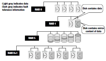
Figure 2-7. RAID configurations
- RAID 0: Striping with no fault tolerance
- RAID 1: Mirroring
- RAID 5: Striping with parity
- RAID 1+0: Striping with mirroring
Raid 0
Since this RAID configuration has no fault tolerance, you can use it only in situations where the reliability of data is not a concern. The failure of any disk in the array will cause complete data loss in the disk subsystem. Therefore, you can’t use it for any data file or transaction log file that constitutes a database, except for the system temporary database called tempdb. The number of I/Os per disk in RAID 0 is represented by the following equation:
I/Os per disk = (Reads + Writes) / Number of disks in the array
In this equation, Reads is the number of read requests to the disk subsystem and Writes is the number of write requests to the disk subsystem.
RAID 1 provides high fault tolerance for critical data by mirroring the data disk onto a separate disk. It can be used where the complete data can be accommodated in one disk only. Database transaction log files for user databases, operating system files, and SQL Server system databases (master and msdb) are usually small enough to use RAID 1.
The number of I/Os per disk in RAID 1 is represented by the following equation:
I/Os per disk =(Reads + 2 X Writes) / 2
RAID 5 is an acceptable option in many cases. It provides reasonable fault tolerance by effectively using only one extra disk to save the computed parity of the data in other disks, as shown in Figure 2-7. When there is a disk failure in RAID 5 configuration, I/O performance becomes terrible, although the system does remain usable while operating with the failed drive.
Any data where writes make up more than 10 percent of the total disk requests is not a good candidate for RAID 5. Thus, use RAID 5 on read-only volumes or volumes with a low percentage of disk writes.
The number of I/Os per disk in RAID 5 is represented by the following equation:
I/Os per disk = (Reads + 4 X Writes) / Number of disks in the array
As shown in this equation, the write operations on the RAID 5 disk subsystem are magnified four times. For each incoming write request, the following are the four corresponding I/O requests on the disk subsystem:
- One read I/O to read existing data from the data disk whose content is to be modified.
- One read I/O to read existing parity information from the corresponding parity disk.
- One write I/O to write the new data to the data disk whose content is to be modified.
- One write I/O to write the new parity information to the corresponding parity disk.
Therefore, the four I/Os for each write request consist of two read I/Os and two write I/Os.
In an OLTP database, all the data modifications are immediately written to the transaction log file as part of the database transaction, but the data in the data file itself is synchronized with the transaction log file content asynchronously in batch operations. This operation is managed by the internal process of SQL Server called the checkpoint process. The frequency of this operation can be controlled by using the recovery interval (min) configuration parameter of SQL Server. Just remember that the timing of checkpoints can be controlled through the use of indirect check points introduced in SQL Server 2012.
Because of the continuous write operation in the transaction log file for a highly transactional OLTP database, placing transaction log files on a RAID 5 array will significantly degrade the array’s performance. Although you should not place the transactional log files on a RAID 5 array, the data files may be placed on RAID 5 since the write operations to the data files are intermittent and batched together to improve the efficiency of the write operation.
Raid 6
RAID 6 is an added layer on top of RAID 5. An extra parity block is added to the storage of RAID 5. This doesn’t negatively affect reads in any way. This means that, for reads, performance is the same as RAID 5. There is an added overhead for the additional write, but it’s not that large. This extra parity block was added because RAID arrays are becoming so large these days that data loss is inevitable. The extra parity block acts as a check against this in order to better ensure that your data is safe.
RAID 1+0 (also referred to as 0+1 and 10) configuration offers a high degree of fault tolerance by mirroring every data disk in the array. It is a much more expensive solution than RAID 5, since double the number of data disks are required to provide fault tolerance. This RAID configuration should be used where a large volume is required to save data and more than 10 percent of disk requests are writes. Since RAID 1+0 supports split seeks (the ability to distribute the read operations onto the data disk and the mirror disk and then converge the two data streams), read performance is also very good. Thus, use RAID 1+0 wherever performance is critical.
The number of I/Os per disk in RAID 1+0 is represented by the following equation:
I/Os per disk = (Reads + 2 X Writes) / Number of disks in the array
Using a SAN System
SANs remain largely the domain of large-scale enterprise systems, although the cost is coming down. A SAN can be used to increase performance of a storage subsystem by simply providing more spindles and disk drives to read from and write to. A “drive” as seen by the operating system is striped across multiple redundant drives in a SAN in a manner similar to that of RAID 5 but without the overhead of RAID 5 or the performance loss caused by disk failures. Because of their size, complexity, and cost, SANs are not necessarily a good solution in all cases. Also, depending on the amount of data, direct attached storage (DAS) can be configured to run faster. The principal strength of SAN systems is not reflected in performance but rather in the areas of scalability, availability, and maintenance.
Another area where SANs are growing are SAN devices that use iSCSI (internet Small Computing System Interface) to connect a device to the network. Because of how the iSCSI interface works, you can make a network device appear to be locally attached storage. In fact, it can work nearly as fast as locally attached storage, but you get to consolidate your storage systems.
Using SSD Disks
Solid State Drives (SSD) are taking the disk performance world by storm. These drives use memory instead of spinning disks to store information. They’re quiet, lower power, and supremely fast. However, they’re also quite expensive when compared to hard disk drives (HDD). At this writing, it costs approximately $.04/GB for a HDD and $1.44/GB for an SSD. But that cost is offset by an increase in speed from approximately 100 operations per second to 5,000 operations per second and up. You can also put SSDs into arrays through a SAN or RAID, further increasing the performance benefits. There are a limited number of write operations possible on an SSD drive, but the failure rate is no higher than that from HDDs so far. For a hardware only solution, implementing SSDs is probably the best operation you can do for a system that is I/O bound.
Aligning Disks Properly
Windows Server 2008 aligns disks as part of the install process, so modern servers should not be running into this issue. However, if you have an older server, this can still be a concern. You’ll also need to worry about this if you’re moving volumes from a pre-Windows Server 2008 system You will need to reformat these in order to get the alignment set appropriately. The way data is stored on a disk is in a series of sectors (also referred to as blocks) that are stored on tracks. A disk is out of alignment when the size of the track, determined by the vendor, consists of a number of sectors different from the default size that you’re writing to. This will mean that one sector will be written correctly, but the next one will have to cross two tracks. This can more than double the amount of I/O required to write or read from the disk. The key is to align the partition so that you’re storing the correct number of sectors for the track.
Adding System Memory
When physical memory is scarce, the system starts writing the contents of memory back to disk and reading smaller blocks of data more frequently, causing a lot of paging. The less memory the system has, the more the disk subsystem is used. This can be resolved using the memory bottleneck resolutions enumerated in the previous section.
Creating Multiple Files and Filegroups
In SQL Server, each user database consists of one or more data files and usually one transaction log file. The data files belonging to a database can be grouped together in one or more filegroups for administrative and data allocation/placement purposes. For example, if a data file is placed in a separate filegroup, then write access to all the tables in the filegroup can be controlled collectively by making the filegroup read-only (transaction log files do not belong to any filegroup).
You can create a filegroup for a database from SQL Server Management Studio, as shown in Figure 2-8. The filegroups of a database are presented in the Filegroups pane of the Database Properties dialog box.
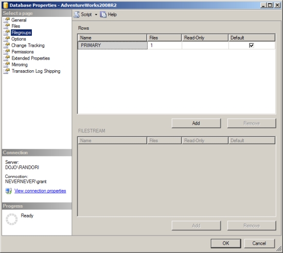
Figure 2-8. Filegroups configuration
In Figure 2-8, you can see that a single filegroup is created by default with AdventureWorks2008. You can add multiple files to multiple filegroups distributed across drives so that work can be done in parallel across the groups and files.
You can add a data file to a filegroup in the Database Properties dialog box in the Files window by selecting from the drop-down list, as shown in Figure 2-9.
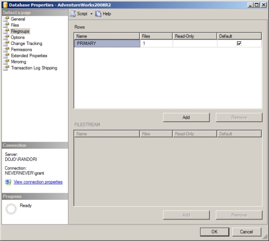
Figure 2-9. Data files configuration
You can also do this programmatically, as follows:
ALTER DATABASE AdventureWorks2008R2 ADD FILEGROUP Indexes ;
ALTER DATABASE AdventureWorks2008R2 ADD FILE (NAME = AdventureWorks2008_Data2j,
FILENAME = 'C:DATAAdventureWorks2008_2.ndf',
SIZE = 1mb,
FILEGROWTH = 10%) TO FILEGROUP Indexes;
Using multiple files and filegroups can help improve the performance of join operations. By separating tables that are frequently joined into separate filegroups and then putting files within the filegroups on separate disks or LUNS, the separated I/O paths can result in improved performance. For example, consider the following query:
SELECT jc.JobCandidateID,
e.ModifiedDate
FROM HumanResources.JobCandidate AS jc
INNER JOIN HumanResoures.Employee AS e
ON jc.BusinessEntityID = e.BusinessEntityID;
If the tables HumanResources.JobCandidate and Person.BusinessEntity are placed in separate filegroups containing one file each, the disks can be read from multiple I/O paths, increasing performance.
It is recommended for performance and recovery purposes that, if multiple filegroups are to be used, the primary filegroup should be used only for system objects and secondary filegroups should be used only for user objects. This approach improves the ability to recover from corruption. The recoverability of a database is higher if the primary data file and the log files are intact. Use the primary filegroup for system objects only, and store all user-related objects on a secondary filegroup.
Spreading a database into multiple files, even on the same drive, makes it easy to move the database files onto separate drives, making future disk upgrades easier. For example, to move a user database file (AdventureWorks2008_2.ndf) to a new disk subsystem (F:), you can follow these steps.
1. Detach the user database as follows :
USE master;
GO
sp_detach_db 'AdventureWorks2008R2';
GO
2. Copy the data file AdventureWorks2008_2.ndf to a folder F:Data on the new disk subsystem.
3. Reattach the user database by referring files at appropriate locations, as shown here:
USE master;
GO
sp_attach_db 'AdventureWorks2008R2'
, 'R:DATAAdventureWorks2008.mdf'
, 'R:DATAAdventureWorks2008_2.ndf'
, 'S:LOGAdventureWorks2008.1df ';
GO
4. To verify the files belonging to a database, execute the following commands:
USE Adventureworks2008R2
GO
SELECT * FROM sys.database_files
GO
Placing the Table and Index on Separate Disks
SQL Server can take advantage of multiple filegroups by accessing tables and corresponding nonclustered indexes using separate I/O paths. A nonclustered index can be created on a specific filegroup as follows:
CREATE INDEX IndexBirthDate
ON HumanResources.Employee (BirthDate)
ON Indexes;
This new index on the HumanResources.Employee table would be created on a filegroup named Indexes.
![]() Tip The nonclustered index and other types of indexes are explained in Chapter 4.
Tip The nonclustered index and other types of indexes are explained in Chapter 4.
Moving the Log Files to a Separate Physical Disk
SQL Server log files should always, when possible, be located on a separate hard disk drive from all other SQL Server database files. Transaction log activity primarily consists of sequential write I/O, unlike the nonsequential (or random) I/O required for the data files. Separating transaction log activity from other nonsequential disk I/O activity can result in I/O performance improvements because it allows the hard disk drives containing log files to concentrate on sequential I/O. But, remember, there are random transaction log reads and the data reads and writes can be sequential as much as the transaction log. There is just a strong tendency of transaction log writes to be sequential.
The major portion of time required to access data from a hard disk is spent on the physical movement of the disk spindle head to locate the data. Once the data is located, the data is read electronically, which is much faster than the physical movement of the head. With only sequential I/O operations on the log disk, the spindle head of the log disk can write to the log disk with a minimum of physical movement. If the same disk is used for data files, however, the spindle head has to move to the correct location before writing to the log file. This increases the time required to write to the log file and thereby hurts performance.
Even with an SSD disk, separating the storage means the work will be distributed to multiple locations, improving the performance.
Furthermore, for SQL Server with multiple OLTP databases, the transaction log files should be physically separated from each other on different physical drives to improve performance. An exception to this requirement is a read-only database or a database with very few database changes. Since no online changes are made to the read-only database, no write operations are performed on the log file. Therefore, having the log file on a separate disk is not required for the read-only databases.
As a general rule of thumb, you should try, where possible, to isolate files with the highest I/O from other files with high I/O. This will reduce contention on the disks and possibly improve performance. To identify those files using the most I/O, reference sys.dm_io_virtual_file_stats.
In addition to simply adding files to filegroups and letting SQL Server distribute the data between them, it’s possible to define a horizontal segmentation of data called a partition so that data is divided up between multiple files by the partition. A filtered set of data is a segment; for example, if the partition is by month, the segment of data is any given month. Creating a partition moves the segment of data to a particular filegroup and only that filegroup. This provides a massive increase in speed because, when querying against well-defined partitions, only the files with the partitions of data you’re interested in will be accessed during a given query. If you assume for a moment that data is partitioned by month, then each month’s data file can be set to read-only as each month ends. That read-only status means that no locking will occur on a file as read queries are run against it, further increasing the performance of your queries. Just remember that partitions are primarily a manageability feature. While you can see some performance benefits from them in certain situations, it shouldn’t be counted on as part of partitioning the data. SQL Server Denali supports up to 15,000 partitions.
SQL Server 2008 makes heavy use of any processor resource available. You can use the Performance Monitor counters in Table 2-4 to analyze pressure on the processor resource.
Table 2-4. Performance Monitor Counters to Analyze CPU Pressure
I’ll now walk you through these counters in more detail.
% Processor Time should not be consistently high (greater than 75 percent). The effect of any sustained processor time greater than 90 percent is the same as that of 100 percent. If % Processor Time is consistently high and disk and network counter values are low, your first priority must be to reduce the stress on the processor. Just remember that the numbers suggested are simply suggestions. Honest people can disagree with these numbers for valid reasons. Use them as a starting point for evaluating your system, not as a hard and fast specific recommendation.
For example, if % Processor Time is 85 percent and % Disk Time is 50 percent, it is quite likely that a major part of the processor time is spent on managing the disk activities. This will be reflected in the % Privileged Time counter of the processor, as explained in the next section. In that case, it will be advantageous to optimize the disk bottleneck first. Further, remember that the disk bottleneck in turn can be because of a memory bottleneck, as explained earlier in the chapter.
You can track processor time as an aggregate of all the processors on the machine, or you can track the percentage utilization individually to particular processors. This allows you to segregate the data collection in the event that SQL Server runs on three processors of a four-processor machine. Remember, you might be seeing one processor maxed out while another processor has very little load. The average value wouldn’t reflect reality in that case.
Processing on a Windows server is done in two modes: user mode and privileged (or kernel] mode. All system-level activities, including disk access, are done in privileged mode. If you find that % Privileged Time on a dedicated SQL Server system is 20 to 25 percent or more, then the system is probably doing a lot of I/O—likely more than you need. The % Privileged Time counter on a dedicated SQL Server system should be at most 5 to 10 percent.
Processor Queue Length is the number of threads in the processor queue. (There is a single processor queue, even on computers with multiple processors.) Unlike the disk counters, the Processor Queue Length counter does not read threads that are already running. On systems with lower CPU utilization, the Processor Queue Length counter is typically 0 or 1.
A sustained Processor Queue Length counter of greater than 2 generally indicates processor congestion. Because of multiple processors, you may need to take into account the number of schedulers dealing with the processor queue length. A processor queue length more than two times the number of schedulers (usually 1:1 with processors) can also indicate a processor bottleneck. Although a high % Processor Time counter indicates a busy processor, a sustained high Processor Queue Length counter is a more certain indicator. If the recommended value is exceeded, this generally indicates that there are more threads ready to run than the current number of processors can service in an optimal way.
The Context Switches/sec counter monitors the combined rate at which all processors on the computer are switched from one thread to another. A context switch occurs when a running thread voluntarily relinquishes the processor, is preempted by a higher-priority ready thread, or switches between user mode and privileged mode to use an executive or a subsystem service. It is the sum of Thread:Context Switches/sec for all threads running on all processors in the computer, and it is measured in numbers of switches.
A figure of 300 to 2,000 Context Switches/sec per processor is excellent to fair. Abnormally high rates, greater than 20,000 per second, can be caused by page faults due to memory starvation.
Batch Requests/sec gives you a good indicator of just how much load is being placed on the system, which has a direct correlation to how much load is being placed on the processor. Since you could see a lot of low-cost queries on your system or a few high-cost queries, you can’t look at this number by itself but must reference the other counters defined in this section; 10,000 requests in a second would be considered a busy system. Greater values may be cause for concern. The best way to know which value has meaning within your own systems is to establish a baseline and then monitor from there. Just remember that a high number here is not necessarily cause for concern. If all your other resources are in hand and you’re sustaining a high number of batch requests/sec, it just means your server is busy.
The SQL Compilations/sec counter shows both batch compiles and statement recompiles as part of its aggregation. This number can be extremely high when a server is first turned on (or after a failover or any other startup type event), but it will stabilize over time. Once stable, spikes in compilations different from a baseline measure is cause for concern and will certainly manifest as problems in the processor. If you are working with some type of object relational mapping engine, such as nHibernate or Entity Framework, a high number of compilations might be normal. Chapter 9 covers SQL compilation in detail.
SQL Recompilations/sec is a measure of the recompiles of both batches and statements. A high number of recompiles will lead to processor stress. Because statement recompiles are part of this count, it can be much higher than in versions of SQL Server prior to 2005. Chapter 10 covers query recompilation in detail.
Other Tools for Measuring CPU Performance
You can use the DMOs to capture information about your CPU as well. The information in these DMOs will have to be captured by running the query and then keeping the information as part of your baseline measurement.
Wait statistics are a good way to understand if there are bottlenecks on the system. You can’t simply say something greater than X is a bad number, though. You need to gather metrics over time in order to understand what represents normal on your system. The deviations from that are interesting. Queries against this DMO that look for signal wait time will be indications of CPU bottlenecks.
Sys.dm_os_workers and Sys.dm_os_schedulers
These DMOs display the worker and scheduler threads within the Windows operating system. Running queries against these regularly will allow you to get counts of the number of processes that are in a runnable state. This is an excellent indication of processor load.
Processor Bottleneck Resolutions
A few of the common processor bottleneck resolutions are as follows:
- Optimizing application workload
- Eliminating or reducing excessive compiles/recompiles
- Using more or faster processors
- Using a large L2/L3 cache
- Running with more efficient controllers/drivers
- Not running unnecessary software
Let’s consider each of these resolutions in turn.
Optimizing Application Workload
To identify the processor-intensive queries, capture all the SQL queries using Extended Events sessions (which I will discuss in the next chapter), and then group the output on the CPU column. The queries with the highest amount of CPU time contribute the most to the CPU stress. You should then analyze and optimize those queries to reduce stress on the CPU. You can also query directly against the sys.dm_exec_query_stats or sys.dm_exec_procedure_stats dynamic management views to see immediate issues in real time. Finally, using both a query hash and a query plan hash, you can identify and tune common queries or common execution plans (this is discussed in detail in Chapter 9). Most of the rest of the chapters in this book are concerned with optimizing application workload.
Eliminating Excessive Compiles/Recompiles
A certain number of query compiles and recompiles is simply to be expected, especially, as already noted, when working with ORM tools. It’s when there is a large number of these over sustained periods that a problem exists. It’s also worth noting the ratio between them. A high number of compiles and a very low number of recompiles means that few queries are being reused within the system (query reuse is covered in detail in Chapter 9). A high number of recompiles will cause high processor use. Methods for addressing recompiles are covered in Chapter 10.
Using More or Faster Processors
One of the easiest resolutions, and one that you will adopt most of the time, is to increase system processing power. However, because of the high cost involved in a processor upgrade, you should first optimize CPU-intensive operations as much as possible.
The system’s processing power can be increased by increasing the power of individual processors or by adding more processors. When you have a high % Processor Time counter and a low Processor Queue Length counter, it makes sense to increase the power of individual processors. In the case of both a high % Processor Time counter and a high Processor Queue Length counter, you should consider adding more processors. Increasing the number of processors allows the system to execute more requests simultaneously.
Using a Large L2/L3 Cache
Modern processors have become so much faster than memory that they need at least two levels of memory cache to reduce latency. On Pentium-class machines, the fast L1 cache holds 8KB of data and 8KB of instructions, while the slower L2 cache holds up to 6MB of mixed code and data. New processors are shipping with an L3 cache on top of the others varying in size from 6MiB to 256MiB and 2MB (MiB refers to mebibyte, a binary representation, 220, that is very similar in size to but not exactly the same as a megabyte, which is 106). References to content found in the L1 cache cost one cycle, references to the L2/L3 cache cost four to seven cycles, and references to the main memory cost dozens of processor cycles. With the increase in processing power, the latter figure will soon exceed 100 cycles. In many ways, the cache is like small, fast, virtual memory inside the processor.
Database engines like L2/L3 caches because they keep processing off the system bus. The processor does not have to go through the system bus to access memory; it can work out of the L2/L3 cache. Not having enough L2/L3 cache can cause the processor to wait a longer period of time for the data/code to move from the main memory to the L2/L3 cache. A processor with a high clock speed but a slow L2/L3 cache may waste a large number of CPU cycles waiting on the small L2/L3 cache. A large L2/L3 cache helps maximize the use of CPU cycles for actual processing instead of waiting on the L2/L3 cache.
Today, it is very common to have megabyte caches on four-way systems. With new four- and eight-way systems, you will often get up to a 6MB L2 cache and, as mentioned earlier, 256MiB on L3. For example, sometimes you may get a performance improvement of 20 percent or more simply by using a 512KB L2 cache instead of a 256KB L2 cache.
Running More Efficient Controllers/Drivers
There is a big difference in % Privileged Time consumption between different controllers and controller drivers on the market today. The techniques used by controller drivers to do I/O are quite different and consume different amounts of CPU time. If you can change to a controller that frees up 4 to 5 percent of % Privileged Time, you can improve performance.
Not Running Unnecessary Software
Corporate policy frequently requires virus checking software be installed on the server. You can also have other products running on the server. When possible, no unnecessary software should be running on the same server as SQL Server. Exterior applications that have nothing to do with maintaining the Windows Server or SQL Server are best placed on a different machine.
In SQL Server OLTP production environments, you find few performance issues that are because of problems with the network. Most of the network issues you face in the OLTP environment are in fact hardware or driver limitations or issues with switches or routers. Most of these issues can be best diagnosed with the Network Monitor tool. However, Performance Monitor also provides objects that collect data on network activity, as shown in Table 2-5.
Table 2-5. Performance Monitor Counters to Analyze Network Pressure
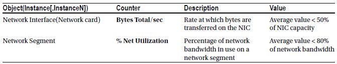
Bytes Total/sec
You can use the Bytes Total/sec counter to determine how the network interface card (NIC) or network adapter is performing. The Bytes Total/sec counter should report high values to indicate a large number of successful transmissions. Compare this value with that reported by the Network InterfaceCurrent Bandwidth performance counter, which reflects each adapter’s bandwidth.
To allow headroom for spikes in traffic, you should usually average no more than 50 percent of capacity. If this number is close to the capacity of the connection and if processor and memory use are moderate, then the connection may well be a problem.
% Net Utilization
The % Net Utilization counter represents the percentage of network bandwidth in use on a network segment. The threshold for this counter depends on the type of network. For Ethernet networks, for example, 30 percent is the recommended threshold when SQL Server is on a shared network hub. For SQL Server on a dedicated full-duplex network, even though near 100 percent usage of the network is acceptable, it is advantageous to keep the network utilization below an acceptable threshold to keep room for the spikes in the load.
![]() Note You must install the Network Monitor Driver to collect performance data using the Network Segment object counters.
Note You must install the Network Monitor Driver to collect performance data using the Network Segment object counters.
In Windows Server 2008, you can install the Network Monitor Driver from the local area connection properties for the network adapter. The Network Monitor Driver is available in the network protocol list of network components for the network adapter.
Network Bottleneck Resolutions
A few of the common network bottleneck resolutions are as follows:
- Optimizing application workload
- Adding network adapters
- Moderating and avoiding interruptions
Let’s consider these resolutions in more detail.
Optimizing Application Workload
To optimize network traffic between a database application and a database server, make the following design changes in the application:
- Instead of sending a long SQL string, create a stored procedure for the SQL query. Then, you just need to send over the network the name of the stored procedure and its parameters.
- Group multiple database requests into one stored procedure. Then, only one database request is required across the network for the set of SQL queries implemented in the stored procedure.
- Request a small data set. Do not request table columns that are not used in the application logic.
- Move data-intensive business logic into the database as stored procedures or database triggers to reduce network round-trips.
- If data doesn’t change frequently, try caching the information on the application instead of frequently calling the database for information that is going to be exactly the same as the last call.
SQL Server Overall Performance
To analyze the overall performance of a SQL Server, besides examining hardware resource utilization, you should also examine some general aspects of SQL Server itself. You can use the performance counters presented in Table 2-6.
Table 2-6 . Performance Monitor Counters to Analyze Generic SQL Pressure
| Object(Instance[,InstanceN]) | Counter |
| SQLServer:Access Methods | FreeSpace Scans/sec Full Scans/sec Table Lock Escalations/sec Worktables Created/sec |
| SQLServer:Latches | Total Latch Wait Time (ms) |
| SQLServer:Locks(_Total) | Lock Timeouts/sec Lock Wait Time (ms) Number of Deadlocks/sec |
| SQLServer:SQL Statistics | Batch Requests/sec SQL Re-Compilations/sec |
| SQLServer:General Statistics | Processes Blocked User Connections Temp Tables Creation Rate Temp Tables for Destruction |
Let’s take a look at each of these counters in context.
To analyze the possibility of missing indexes causing table scans or large data set retrievals, you can use the counter in Table 2-7.
Table 2-7. Performance Monitor Counter to Analyze Excessive Data Scans
| Object(Instance[,InstanceN]) | Counter |
| SQLServer:Access Methods | Full Scans/sec |
This counter monitors the number of unrestricted full scans on base tables or indexes. A few of the main causes of high Full Scans/sec are as follows:
- Missing indexes
- Too many rows requested
To further investigate queries producing these problems, use SQL Profiler to identify the queries (I will cover this tool in the next chapter). Queries with missing indexes or too many rows requested will have a large number of logical reads and an increased CPU time.
Be aware of the fact that full scans may be performed for the temporary tables used in a stored procedure, because most of the time you will not have indexes (or you will not need indexes) on temporary tables. Still, adding this counter to the baseline helps identify the possible increase in the use of temporary tables, which are usually not good for performance.
Dynamic Management Objects
Another way to check for missing indexes is to query the dynamic management view sys.dm_db_missing_index_details. This management view returns information that can suggest candidates for indexes based on the execution plans of the queries being run against the database. The view sys.dm_db_missing_index_details is part of a series of DMVs collectively referred to as the missing indexes feature. These DMVs are based on data generated from execution plans stored in the cache. You can query directly against this view to gather data to decide whether you want to build indexes based on the information available from within the view. Missing indexes will also be shown within the XML execution plan for a given query, but I’ll cover that more in the next chapter. While these views are useful for suggesting possible indexes, since they can’t be linked to a particular query, you must test these suggestions prior to implementing them on your systems.
The opposite problem to a missing index is one that is never used. The DMV sys.dm_db_index_usage_stats shows which indexes have been used, at least since the last reboot of the system. You can also view the indexes in use with a lower-level DMV, sys.dm_db_index_operational_stats. It will help to show where indexes are slowing down because of contention or I/O. I’ll cover these both in more detail in Chapter 10. You may also find that the suggestions from the Database Tuning Advisor can help you with specific indexes for specific queries.
To analyze the impact of database blocking on the performance of SQL Server, you can use the counters shown in Table 2-8.
Table 2-8 . Performance Monitor Counters to Analyze SQL Server Locking
|
Object(lnstance[,lnstanceN]) |
Counter |
| SQLServer:Latches | Total Latch Wait Time (ms) |
| SQLServer:Locks(_Total) |
Lock Timeouts/sec
Lock Wait Time (ms) Number of Deadlocks/sec |
Latches are used internally by SQL Server to protect the integrity of internal structures, such as a table row, and are not directly controlled by users. This counter monitors total latch wait time (in milliseconds) for latch requests that had to wait in the last second. A high value for this counter indicates that SQL Server is spending too much time waiting on its internal synchronization mechanism.
Lock timeouts/sec and Lock Wait time (ms)
You should expect Lock Timeouts/sec to be 0 and Lock Wait Time (ms) to be very low. A nonzero value for Lock Timeouts/sec and a high value for Lock Wait Time (ms) indicate that excessive blocking is occurring in the database. Two approaches can be adopted in this case.
- You can identify the costly queries using data from SQL Profiler or by querying sys. dm_execquerystats and then optimize the queries appropriately.
- You can use blocking analysis to diagnose the cause of excessive blocking. It is usually advantageous to concentrate on optimizing the costly queries first, because this, in turn, reduces blocking for others. In Chapter 12, you will learn how to analyze and resolve blocking.
Just remember that some degree of locks are a necessary part of the system. You’ll want to establish a baseline in order to track thoroughly if a given value is cause for concern.
You should expect to see a 0 value for this counter. If you find a nonzero value, then you should identify the victimized request and either resubmit the database request automatically or suggest that the user do so. More importantly, an attempt should be made to troubleshoot and resolve the deadlock. Again, Chapter 12 shows how to do this.
Since generating an execution plan for a stored procedure query requires CPU cycles, you can reduce the stress on the CPU by reusing the execution plan. To analyze the number of stored procedures that are recompiling, you can look at the counter in Table 2-9.
Table 2-9. Performance Monitor Counter to Analyze Execution Plan Reusability
| Object(lnstance[,lnstanceN]) | Counter |
| SQLServer:SOL Statistics | SOL Re-Compilations/sec |
Recompilations of stored procedures add overhead on the processor. You want to see a value close to 0 for the SOL Re-Compilations/sec counter. If you consistently see nonzero values, then you should use Extended Events to further investigate the stored procedures undergoing recompilations. Once you identify the relevant stored procedures, you should attempt to analyze and resolve the cause of recompilations. In Chapter 10, you will learn how to analyze and resolve various causes of recompilation.
General Behavior
SQL Server provides additional performance counters to track some general aspects of a SQL Server system. Table 2-10 lists a few of the most commonly used counters.
Table 2-10 . Performance Monitor Counters to Analyze Volume of Incoming Requests
| Object(Instance[,InstanceN]) | Counter |
| SQLServer:General Statistics | User Connections |
| SQLServer:SQL Statistics | Batch Requests/sec |
Multiple read-only SQL Servers can work together in a load-balancing environment (where SQL Server is spread over several machines) to support a large number of database requests. In such cases, it is better to monitor the User Connections counter to evaluate the distribution of user connections across multiple SQL Server instances. User Connections can range all over the spectrum with normal application behavior. This is where a normal baseline is essential to determine the expected behavior. You will see how you can establish this baseline shortly.
This counter is a good indicator of the load on SQL Server. Based on the level of system resource utilization and Batch Requests/sec, you can estimate the number of users SQL Server may be able to take without developing resource bottlenecks. This counter value, at different load cycles, helps you understand its relationship with the number of database connections. This also helps you understand SQL Server’s relationship with Web Request/sec, that is, Active Server Pages.Requests/sec for web applications using Microsoft Internet Information Services (IIS) and Active Server Pages (ASP). All this analysis helps you better understand and predict system behavior as the user load changes.
The value of this counter can range over a wide spectrum with normal application behavior. A normal baseline is essential to determine the expected behavior.
Considerations for Monitoring Virtual Machines
When you are working with Virtual Machines (VM) many of the standard performance metrics counters are no longer applicable. If you monitor these counters within the VM, you will be getting very unrealistic numbers.
If you monitor these counters on the physical box, which doubtless is shared by multiple different VMs, you will be unable to identify specific SQL Server instance resource bottlenecks. Because of this, additional information must be monitored when working with a VM. Most of the information that you can gather on disk and network performance are still applicable within a VM setting. It’s the memory and CPU metrics that are completely different.
This is because CPU and memory are shared between machines within a virtualized server environment. You may start a process on one CPU and finish it on another one entirely. Some virtual environments can actually change the memory allocated to a machine as that machine’s demands for memory go up and down. With these kinds of changes, traditional monitoring just isn’t applicable. The good news is that the major VM vendors provide you with guidance on how to monitor their systems and how to use SQL Server within their systems. You can largely rely on these third party documents for the specifics of monitoring a VM.
The queues counters, such as processor queue length, are still applicable when monitoring within a VM. These indicate that the VM itself is starved for resources, starving your SQL Server instance so that it has to wait for access to the virtual CPU. The important thing to remember is, CPU and memory are going to be slower on a VM because of the management of the VM getting in the way of the system resources.
Now that you have looked at a few of the main performance counters, let’s see how to bring these counters together to create a system baseline. These are the steps you need to follow:
1. Create a reusable list of performance counters.
2. Create a counter log using your list of performance counters.
3. Minimize Performance Monitor overhead.
Creating a Reusable List of Performance Counters
Run the Performance Monitor tool on a Windows Server 2008 machine connected to the same network as that of the SQL Server system. Add performance counters to the View Chart display of the Performance Monitor through the Properties ![]() Data
Data ![]() Add Counters dialog box, as shown in Figure 2-10.
Add Counters dialog box, as shown in Figure 2-10.
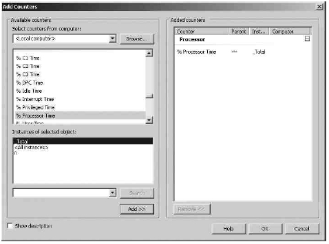
Figure 2-10. Adding Performance Monitor counters
For example, to add the performance counter Processor(_Total)\% Processor Time, follow these steps:
1. Select the option Select Counters from Computer and specify the computer name running SQL Server in the corresponding entry field.
2. Click the box next to the performance object Processor.
3. Choose the % Processor Time counter from the list of performance counters.
4. Choose instance Total from the instances in the Instances of Selected Object list.
5. Click the Add button to add this performance counter to the list of counters to be added.
6. Continue as needed with other counters. When finished, click the OK button.
When creating a reusable list for your baseline, you can repeat the preceding steps to add all the performance counters listed in Table 2-11.
Table 2-11 . Performance Monitor Counters to Analyze SQL Server Performance
| Object(lnstance[,lnstanceN]) | Counter |
| Memory | Available Mbytes Pages/sec |
| PhysicalDisk(Data-disk, Log-disk) | % Disk Time Current Disk Queue Length Disk Transfers/sec Disk Bytes/sec |
| Processor(_Total) | % Processor Time % Privileged Time |
| System | Processor Queue Length Context Switches/sec |
| Network Interface(Network card) | Bytes Total/sec |
| Network Segment | % Net Utilization |
| SQLServer:Access Methods | FreeSpace Scans/sec Full Scans/sec |
| SQLServer:Buffer Manager | Buffer cache hit ratio Free pages |
| SQLServer:Latches | Total Latch Wait Time (ms) |
| SQLServer:Locks(_Total) | Lock Timeouts/sec Lock Wait Time (ms) Number of Deadlocks/sec |
| SQLServer:Memory Manager | Memory Grants Pending Target Server Memory (KB) Total Server Memory (KB) |
| SQLServer:SQL Statistics | Batch Requests/sec SQL Re-Compilations/sec |
| SQLServer:General Statistics | User Connections |
Once you have added all the performance counters, close the Add Counters dialog box. To save the list of counters as an .htm file, right-click anywhere in the right frame of Performance Monitor, and select the Save Settings As menu item.
The .htm file lists all the performance counters that can be used as a base set of counters to create a counter log or to view Performance Monitor graphs interactively for the same SQL Server machine. To use this list of counters for other SQL Server machines, open the .htm file in an editor such as Notepad, and replace all instances of \SQLServerMachineName with ‘’ (a blank string), without the quotes.
You can also use this counter list file to view Performance Monitor graphs interactively in an Internet browser, as shown in Figure 2-11.
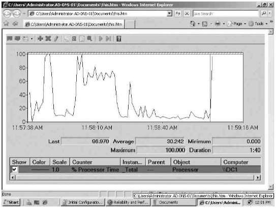
Figure 2-11. Performance Monitor in Internet browser
Creating a Counter Log Using the List of Performance Counters
Performance Monitor provides a counter log facility to save the performance data of multiple counters over a period of time. You can view the saved counter log using Performance Monitor to analyze the performance data. It is usually convenient to create a counter log from a defined list of performance counters. Simply collecting the data rather than viewing it through the GUI is the preferred method of automation to prepare for troubleshooting your server’s performance or establishing a baseline.
Expand Data Collector Sets ![]() User Defined. Right-click, and select New
User Defined. Right-click, and select New ![]() Data Collector Set. Define the name of the set, and make this a manual creation by clicking the appropriate radio button; then click Next. You’ll have to define what type of data you’re collecting. In this case, select the check box Performance Counters under the Create Data Logs radio button, and then click Next. Here you can define the performance objects you want to collect using the same Add Counters dialog box shown earlier in Figure 2-10. Clicking Next allows you to define the destination folder. Click Next, then select the radio button Open Properties for This Data Collector Set, and click Finish. You can schedule the counter log to automatically start at a specific time and stop after a certain time period or at a specific time. You can configure these settings through the Schedule pane. Figure 2-12 shows the summary of which counters have been selected as well as the frequency with which the counters will be collected.
Data Collector Set. Define the name of the set, and make this a manual creation by clicking the appropriate radio button; then click Next. You’ll have to define what type of data you’re collecting. In this case, select the check box Performance Counters under the Create Data Logs radio button, and then click Next. Here you can define the performance objects you want to collect using the same Add Counters dialog box shown earlier in Figure 2-10. Clicking Next allows you to define the destination folder. Click Next, then select the radio button Open Properties for This Data Collector Set, and click Finish. You can schedule the counter log to automatically start at a specific time and stop after a certain time period or at a specific time. You can configure these settings through the Schedule pane. Figure 2-12 shows the summary of which counters have been selected as well as the frequency with which the counters will be collected.
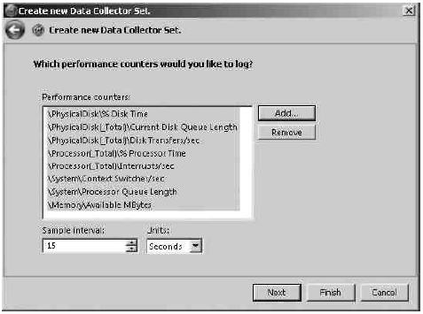
Figure 2-12. Defining a Performance Monitor counter log
![]() Tip I’ll offer additional suggestions for these settings in the section that follows.
Tip I’ll offer additional suggestions for these settings in the section that follows.
For additional information on how to create counter logs using Performance Monitor, please refer to the Microsoft Knowledge Base article “Performance Tuning Guidelines for Windows Server 2008” at http://download.microsoft.com/download/9/c/5/9c5b2167-8017-4bae-9fde-d599bac8184a/Perf-tun-srv.docx .
Performance Monitor Considerations
The Performance Monitor tool is designed to add as little overhead as possible, if used correctly. To minimize the impact of using this tool on a system, consider the following suggestions:
- Limit the number of counters, specifically performance objects.
- Use counter logs instead of viewing Performance Monitor graphs interactively.
- Run Performance Monitor remotely while viewing graphs interactively.
- Save the counter log file to a different local disk.
- Increase the sampling interval.
Let’s consider each of these points in more detail.
Limit the Number of Counters
Monitoring large numbers of performance counters with small sampling intervals could incur some amount of overhead on the system. The bulk of this overhead comes from the number of performance objects you are monitoring, so selecting them wisely is important. The number of counters for the selected performance objects does not add much overhead, because it gives only an attribute of the object itself. Therefore, it is important to know what objects you want to monitor and why.
Prefer Counter Logs
Use counter logs instead of viewing a Performance Monitor graph interactively, because Performance Monitor graphing is more costly in terms of overhead. Monitoring current activities should be limited to short-term viewing of data, troubleshooting, and diagnosis. Performance data reported via a counter log is sampled, meaning that data is collected periodically rather than traced, whereas the Performance Monitor graph is updated in real time as events occur. Using counter logs will reduce that overhead.
View performance Monitor Graphs remotely
Since viewing the live performance data using Performance Monitor graphs creates a fair amount of overhead on the system, run the tool remotely on a different machine and connect to the SQL Server system through the tool. To remotely connect to the SQL Server machine, run the Performance Monitor tool on a machine connected to the network to which the SQL Server machine is also connected.
As shown in Figure 2-10, type the computer name (or IP address) of the SQL Server machine in the Select Counters from Computer box. Be aware that if you connect to the production server through a Windows Server 2008 terminal service session, the major part of the tool will still run on the server.
Save Counter Log Locally
Collecting the performance data for the counter log does not incur the overhead of displaying any graph. So, while using counter log mode, it is more efficient to log counter values locally on the SQL Server system instead of transferring the performance data across the network. Put the counter log file on a local disk other than the ones that are monitored.
Increase the Sampling Interval
Because you are mainly interested in the resource utilization pattern during baseline monitoring, you can easily increase the performance data sampling interval to 60 seconds or more to decrease the log file size and reduce demand on disk I/Os. You can use a short sampling interval to detect and diagnose timing issues. Even while viewing Performance Monitor graphs interactively, increase the sampling interval from the default value of one second per sample. Just remember, changing the sampling size up or down can affect the granularity of the data as well as the quantity. You have to weigh these choices carefully.
System Behavior Analysis Against Baseline
The default behavior of a database application changes over time because of various factors such as the following:
- Data volume and distribution changes
- Increased user base
- Change in usage pattern of the application
- Additions to or changes in the application’s behavior
- Installation of new service packs or software upgrades
- Changes to hardware
Because of these changes, the baseline created for the database server slowly loses its significance. It may not always be accurate to compare the current behavior of the system with an old baseline. Therefore, it is important to keep the baseline current creating a new baseline at regular time intervals. It is also beneficial to archive the previous baseline logs so that they can be referred to later, if required. So while, yes, older baselines are not applicable to day-to-day operations, they do help you in establishing patterns and long term trends.
The counter log for the baseline or the current behavior of the system can be analyzed using the Performance Monitor tool by following these steps:
1. Open the counter log. Use Performance Monitor’s toolbar item View Log File Data, and select the log file name.
2. Add all the performance counters to analyze the performance data. Note that only the performance objects, counters, and instances selected during the counter log creation are shown in the selection lists.
3. Analyze the system behavior at different parts of the day by adjusting the time range accordingly, as shown in Figure 2-13.
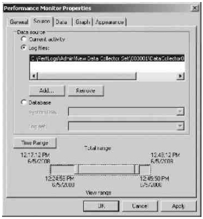
Figure 2-13. Defining time range for log analysis
During a performance review, you can analyze the system-level behavior of the database by comparing the current value of performance counters with the latest baseline. Take the following considerations into account while comparing the performance data:
- Use the same set of performance counters in both cases.
- Compare the minimum, maximum, or average value of the counters as applicable for the individual counters. I explained the specific values for the counters earlier.
- Some counters have an absolute good/bad value, as mentioned previously. The current value of these counters need not be compared with the baseline values. For example, if the current average value of the Pages/sec counter is 100, it indicates that the system has developed a memory bottleneck. Even though it does not require a comparison with the baseline, it is still advantageous to review the corresponding baseline value, because the memory bottleneck might have existed for a long time. Having the archived baseline logs helps detect the first occurrence of the memory bottleneck.
- Some counters do not have a definitive good/bad value. Because their value depends on the application, a relative comparison with the corresponding baseline counters is a must. For example, the current value of the User Connections counter for SQL Server does not signify anything good or bad with the application. But comparing it with the corresponding baseline value may reveal a big increase in the number of user connections, indicating an increase in the workload.
- Compare a range of values for the counters from the current and the baseline counter logs. The fluctuation in the individual values of the counters will be normalized by the range of values.
- Compare logs from the same part of the day. For most applications, the usage pattern varies during different parts of the day. To obtain the minimum, maximum, and average value of the counters for a specific time, adjust the time range of the counter logs as shown previously.
Once the system-level bottleneck is identified, the internal behavior of the application should be analyzed to determine the cause of the bottleneck. Identifying and optimizing the source of the bottleneck will help use the system resources efficiently.
Summary
In this chapter, you learned how to use the Performance Monitor tool to analyze the overall behavior of SQL Server as well as the effect of a slow-performing database application on system resources. For every resultant system bottleneck, there are two types of resolutions: hardware resolutions and application optimization. Of course, it is always beneficial to optimize the database application before considering a hardware upgrade.
In the next chapter, you will learn how to analyze the workload of a database application for performance tuning.