Chapter 11
![]()
Query Design Analysis
A database schema may include a number of performance-enhancement features such as indexes, statistics,
and stored procedures. But none of these features guarantees good performance if your queries are written badly in the first place. The SQL queries may not be able to use the available indexes effectively. The structure of the SQL queries may add avoidable overhead to the query cost. Queries may be attempting to deal with data in a
row-by-row fashion (or to quote Jeff Moden, Row By Agonizing Row, which is abbreviated to RBAR and pronounced “reebar”) instead of in logical sets. To improve the performance of a database application, it is important to understand the cost associated with varying ways of writing a query.
In this chapter, I cover the following topics:
- Aspects of query design that affect performance
- How query designs use indexes effectively
- The role of optimizer hints on query performance
- The role of database constraints on query performance
- Query designs that are less resource-intensive
- Query designs that use the procedure cache effectively
- Query designs that reduce network overhead
- Techniques to reduce the transaction cost of a query
Query Design Recommendations
When you need to run a query, you can often use many different approaches to get the same data. In many cases, the optimizer generates the same plan, irrespective of the structure of the query. However, in some situations the query structure won’t allow the optimizer to select the best possible processing strategy. It is important that you know when this happens and what you can do to avoid it.
In general, keep the following recommendations in mind to ensure the best performance:
- Operate on small result sets.
- Use indexes effectively.
- Avoid optimizer hints.
- Use domain and referential integrity.
- Avoid resource-intensive queries.
- Reduce the number of network round-trips.
- Reduce the transaction cost.
Careful testing is essential to identify the query form that provides the best performance in a specific database environment. You should be conversant with writing and comparing different SQL query forms so you can evaluate the query form that provides the best performance in a given environment.
Operating on Small Result Sets
To improve the performance of a query, limit the amount of data it operates on, including both columns and rows. Operating on a small result set reduces the amount of resources consumed by a query and increases the effectiveness of indexes. Two of the rules you should follow to limit the data set’s size are as follows:
- Limit the number of columns in the select list.
- Use highly selective WHERE clauses to limit the rows returned.
It’s important to note that you will be asked to return tens of thousands of rows to an OLTP system. Just because someone tells you those are the business requirements doesn’t mean they are right. Human beings don’t process tens of thousands of rows. Very few human beings are capable of processing thousands of rows. Be prepared to push back on these requests, and be able to justify your reasons.
Limit the Number of Columns in select_list
Use a minimum set of columns in the select list of a SELECT statement. Don’t use columns that are not required in the output result set. For instance, don’t use SELECT * to return all columns. SELECT * statements render covered indexes ineffective, since it is impractical to include all columns in an index. For example, consider the following query:
SELECT [Name],
TerritoryID
FROM Sales.SalesTerritory AS st
WHERE st.[Name] = 'Australia' ;
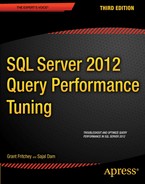
A covering index on the Name column (and through the clustered key, ProductID) serves the query quickly through the index itself, without accessing the clustered index. When you have STATISTICS 10 and STATISTICS TIME switched on, you get the following number of logical reads and execution time, as well as the corresponding execution plan (shown in Figure 11-1):
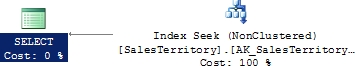
Figure 11-1. Execution plan showing the benefit of referring to a limited number of columns
Table 'SalesTerritory'. Scan count 0, logical reads 2
CPU time = 0 ms, elapsed time = 0 ms.
If this query is modified to include all columns in the select list as follows, then the previous covering index becomes ineffective, because all the columns required by this query are not included in that index:
SELECT *
FROM Sales.SalesTerritory AS st
WHERE st.[Name] = 'Australia' ;
Subsequently, the base table (or the clustered index) containing all the columns has to be accessed, as shown next. The number of logical reads and the execution time have both increased.
Table 'SalesTerritory'. Scan count 0, logical reads 4 CPU time = 0 ms, elapsed time = 75 ms
As shown in Figure 11-2, the fewer the columns in the select list, the better the query performance. Selecting too many columns also increases data transfer across the network, further degrading performance.
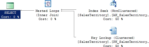
Figure 11-2. Execution plan showing the added cost of referring to too many columns
Use Highly Selective WHERE Clauses
As explained in Chapter 4, the selectivity of a column referred to in the WHERE clause governs the use of an index on the column. A request for a large number of rows from a table may not benefit from using an index, either because it can’t use an index at all or, in the case of a non-clustered index, because of the overhead cost of the bookmark lookup. To ensure the use of indexes, the columns referred to in the WHERE clause should be highly selective.
Most of the time, an end user concentrates on a limited number of rows at a time. Therefore, you should design database applications to request data incrementally as the user navigates through the data. For applications that rely on a large amount of data for data analysis or reporting, consider using data analysis solutions such as Analysis Services. Remember, returning huge result sets is costly, and this data is unlikely to be used in its entirety
Using Indexes Effectively
It is extremely important to have effective indexes on database tables to improve performance. However, it is equally important to ensure that the queries are designed properly to use these indexes effectively. These are some of the query design rules you should follow to improve the use of indexes:
- Avoid nonsargable search conditions.
- Avoid arithmetic operators on the WHERE clause column.
- Avoid functions on the WHERE clause column.
I cover each of these rules in detail in the following sections.
Avoid Nonsargable Search Conditions
A sargable predicate in a query is one in which an index can be used. The word is a contraction of “Search ARGument ABLE.” The optimizer’s ability to benefit from an index depends on the selectivity of the search condition, which in turn depends on the selectivity of the column(s) referred to in the WHERE clause. The search predicate used on the column(s) in the WHERE clause determines whether an index operation on the column can be performed.
The sargable search conditions listed in Table 11-1 generally allow the optimizer to use an index on the column(s) referred to in the WHERE clause. The sargable search conditions generally allow SQL Server to seek to a row in the index and retrieve the row (or the adjacent range of rows until the search condition remains true).
Table 11-1. Common Sargable and Nonsargable Search Conditions
|
Type |
Search Conditions |
|
Sargable |
Inclusion conditions =,>,>=,<,<=, and BETWEEN, and some LIKE conditions such as LIKE '<literal>%' |
|
Nonsargable |
Exclusion conditions <>,!=,!>,!<, NOT EXISTS, NOT IN, and N0T LIKE IN, OR, and some LIKE conditions such as LIKE '%<literal>' |
On the other hand, the nonsargable search conditions listed in Table 11-1 generally prevent the optimizer from using an index on the column(s) referred to in the WHERE clause. The exclusion search conditions generally don’t allow SQL Server to perform Index Seek operations as supported by the sargable search conditions. For example, the != condition requires scanning all the rows to identify the matching rows.
Try to implement workarounds for these nonsargable search conditions to improve performance. In some cases, it may be possible to rewrite a query to avoid a nonsargable search condition. For example, consider replacing an IN/OR search condition with a BETWEEN condition, as described in the following section.
Consider the following query, which uses the search condition IN:
SELECT sod.*
FROM Sales.SalesOrderDetail AS sod
WHERE sod.SalesOrderID IN (51825, 51826, 51827, 51828) ;
You can replace the nonsargable search condition in this query with a BETWEEN clause as follows:
SELECT sod.*
FROM Sales.SalesOrderDetail AS sod
WHERE sod.SalesOrderID BETWEEN 51825 AND 51828 ;
On the face of it, the execution plan of both the queries appears to be the same, as shown in Figure 11-3.
Figure 11-3. Execution plan for a simple SELECT statement using a BETWEEN clause
However, a closer look at the execution plans reveals the difference in their data-retrieval mechanism, as shown in Figure 11-4. The left box is the IN condition, and the right box is the BETWEEN condition.
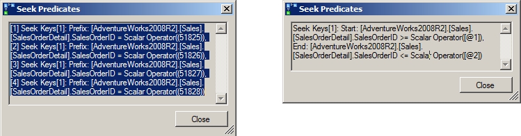
Figure 11-4. Execution plan details for an IN condition (left) and a BETWEEN condition (right)
As shown in Figure 11-4, SQL Server resolved the IN condition containing four values into four OR conditions. Accordingly, the clustered index (PKSalesTerritoryTerritoryld) is accessed four times (Scan count 4) to retrieve rows for the four OR conditions, as shown in the following corresponding STATISTICS 10 output. On the other hand, the BETWEEN condition is resolved into a pair of >= and <= conditions, as shown in Figure 11-4. SQL Server accesses the clustered index only once (Scan count 1) from the first matching row until the match condition is true, as shown in the following corresponding STATISTICS10 and QUERY TIME output.
- With the IN condition:
Table 'SalesOrderDetail'. Scan count 4, logical reads 21
CPU time = 0 ms, elapsed time = 264 ms.
- With the BETWEEN condition:
Table 'SalesOrderDetail'. Scan count 1, logical reads 7
CPU time = 0 ms, elapsed time = 212 ms.
Replacing the search condition IN with BETWEEN decreases the number of logical reads for this query from 21 to 7. As just shown, although both queries use a clustered index seek on OrderID, the optimizer locates the range of rows much faster with the BETWEEN clause than with the IN clause. The same thing happens when you look at the BETWEEN condition and the OR clause. Therefore, if there is a choice between using IN/OR and the BETWEEN search condition, always choose the BETWEEN condition because it is generally much more efficient than the
IN/OR condition. In fact, you should go one step further and use the combination of >= and <= instead of the BETWEEN clause only because you’re making the optimizer do a little less work.
Not every WHERE clause that uses exclusion search conditions prevents the optimizer from using the index on the column referred to in the search condition. In many cases, the SQL Server 2012 optimizer does a wonderful job of converting the exclusion search condition to a sargable search condition. To understand this, consider the following two search conditions, which I discuss in the sections that follow:
- The LIKE condition
- The !< condition vs. the >= condition
While using the LIKE search condition, try to use one or more leading characters in the WHERE clause if possible. Using leading characters in the LIKE clause allows the optimizer to convert the LIKE condition to an index-friendly search condition. The greater the number of leading characters in the LIKE condition, the better the optimizer is able to determine an effective index. Be aware that using a wildcard character as the leading character in the LIKE condition prevents the optimizer from performing a SEEK (or a narrow-range scan) on the index; it relies on scanning the complete table instead.
To understand this ability of the SQL Server 2012 optimizer, consider the following SELECT statement that uses the LIKE condition with a leading character:
SELECT c.CurrencyCode
FROM Sales.Currency AS c
WHERE c.[Name] LIKE 'Ice%' ;
The SQL Server 2012 optimizer does this conversion automatically, as shown in Figure 11-5.
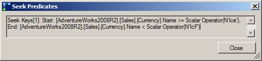
Figure 11-5. Execution plan showing automatic conversion of a LIKE clause with a trailing % sign to an indexable search condition
As you can see, the optimizer automatically converts the LIKE condition to an equivalent pair of >= and < conditions. You can therefore rewrite this SELECT statement to replace the LIKE condition with an indexable search condition as follows:
SELECT c.CurrencyCode
FROM Sales.Currency AS c
WHERE c.[Name] >= N'Ice'
AND c.[Name] < N'IcF' ;
Note that, in both cases, the number of logical reads, the execution time for the query with the LIKE condition, and the manually converted sargable search condition are all the same. Thus, if you include leading characters in the LIKE clause, the SQL Server 2012 optimizer optimizes the search condition to allow the use of indexes on the column.
Even though both the !< and >= search conditions retrieve the same result set, they may perform different operations internally. The >= comparison operator allows the optimizer to use an index on the column referred to in the search argument because the = part of the operator allows the optimizer to seek to a starting point in the index and access all the index rows from there onward. On the other hand, the !< operator doesn’t have an = element and needs to access the column value for every row.
Or does it? As explained in Chapter 9, the SQL Server optimizer performs syntax-based optimization, before executing a query, to improve performance. This allows SQL Server to take care of the performance concern with the !< operator by converting it to >=, as shown in the execution plan in Figure 11-6 for the two following SELECT statements:
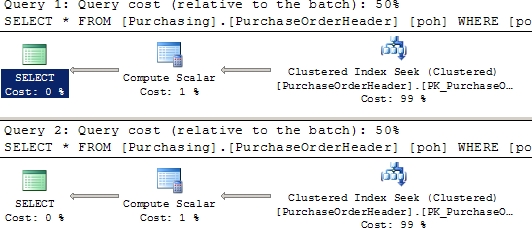
Figure 11-6. Execution plan showing automatic transformation of a nonindexable !< operator to an indexable >= operator
SELECT *
FROM Purchasing.PurchaseOrderHeader AS poh
WHERE poh.PurchaseOrderID >= 2975 ;
SELECT *
FROM Purchasing.PurchaseOrderHeader AS poh
WHERE poh.PurchaseOrderID !< 2975 ;
As you can see, the optimizer often provides you with the flexibility of writing queries in the preferred T-SQL syntax without sacrificing performance.
Although the SQL Server optimizer can automatically optimize query syntax to improve performance in many cases, you should not rely on it to do so. It is a good practice to write efficient queries in the first place.
Avoid Arithmetic Operators on the WHERE Clause Column
Using an arithmetic operator on a column in the WHERE clause can prevent the optimizer from using the index on the column. For example, consider the following SELECT statement:
SELECT *
FROM Purchasing.PurchaseOrderHeader AS poh
WHERE poh.PurchaseOrderID * 2 = 3400 ;
A multiplication operator, *, has been applied on the column in the WHERE clause. You can avoid this on the column by rewriting the SELECT statement as follows:
SELECT *
FROM Purchasing.PurchaseOrderHeader AS poh
WHERE poh.PurchaseOrderID = 3400 / 2 ;
The table has a clustered index on the PurchaseOrderID column. As explained in Chapter 4, an Index Seek operation on this index is suitable for this query since it returns only one row. Even though both queries return the same result set, the use of the multiplication operator on the PurchaseOrderID column in the first query prevents the optimizer from using the index on the column, as you can see in Figure 11-7.
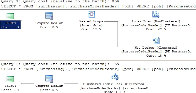
Figure 11-7. Execution plan showing the detrimental effect of an arithmetic operator on a WHERE clause column
The following are the corresponding STATISTICS IO and TIME outputs.
- With the * operator on the PurchaseOrderID column:
Table ‘PurchaseOrderHeader’. Scan count 1, logical reads 11 CPU time = 0 ms, elapsed time = 201 ms.
- With no operator on the PurchaseOrderID column:
Table ‘PurchaseOrderHeader’. Scan count 0, logical reads 2 CPU time = 0 ms, elapsed time =75 ms.
Therefore, to use the indexes effectively and improve query performance, avoid using arithmetic operators on column(s) in the WHERE clause or JOIN criteria when that expression is expected to work with an index.
![]() Note For small result sets, even though an index seek is usually a better data-retrieval strategy than a table scan (or a complete clustered index scan), for very small tables (in which all data rows fit on one page) a table scan can be cheaper. I explain this in more detail in Chapter 4.
Note For small result sets, even though an index seek is usually a better data-retrieval strategy than a table scan (or a complete clustered index scan), for very small tables (in which all data rows fit on one page) a table scan can be cheaper. I explain this in more detail in Chapter 4.
Avoid Functions on the WHERE Clause Column
In the same way as arithmetic operators, functions on WHERE clause columns also hurt query performance—and for the same reasons. Try to avoid using functions on WHERE clause columns, as shown in the following two examples:
- SUBSTRING vs. LIKE
- Date part comparison
In the following SELECT statement (substring.sql in the download), using the SUBSTRING function prevents the use of the index on the ShipPostalCode column.
SELECT d.Name
FROM HumanResources.Department AS d
WHERE SUBSTRING(d.[Name], 1, 1) = 'F' ;
Figure 11-8 illustrates this.
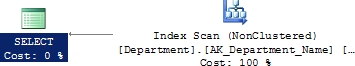
Figure 11-8. Execution plan showing the detrimental effect of using the SUBSTRING function on a WHERE clause column
As you can see, using the SUBSTRING function prevented the optimizer from using the index on the [Name] column. This function on the column made the optimizer use a clustered index scan. In the absence of the clustered index on the DepartmentID column, a table scan would have been performed.
You can redesign this SELECT statement to avoid the function on the column as follows:
SELECT d.Name
FROM HumanResources.Department AS d
WHERE d.[Name] LIKE 'F%' ;
This query allows the optimizer to choose the index on the [Name] column, as shown in Figure 11-9.
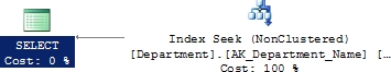
Figure 11-9. Execution plan showing the benefit of not using the SUBSTRING function on a WHERE clause column
Date Part Comparison
SQL Server can store date and time data as separate fields or as a combined DATETIME field that has both. Although you may need to keep date and time data together in one field, sometimes you want only the date, which usually means you have to apply a conversion function to extract the date part from the DATETIME data type. Doing this prevents the optimizer from choosing the index on the column, as shown in the following example.
First, there needs to be a good index on the DATETIME column of one of the tables. Use Sales.SalesOrderHeader and create the following index:
IF EXISTS ( SELECT *
FROM sys.indexes
WHERE object_id = OBJECT_ID(N'[Sales].[SalesOrderHeader]')
AND name = N'IndexTest' )
DROP INDEX IndexTest ON [Sales].[SalesOrderHeader] ;
GO
CREATE INDEX IndexTest ON Sales.SalesOrderHeader(OrderDate) ;
To retrieve all rows from Sales.SalesOrderHeader with OrderDate in the month of April in the year 2008, you can execute the following SELECT statement (datetime.sql):
SELECT soh.SalesOrderID,
soh.OrderDate
FROM Sales.SalesOrderHeader AS soh
JOIN Sales.SalesOrderDetail AS sod
ON soh.SalesOrderID = sod.SalesOrderID
WHERE DATEPART(yy, soh.OrderDate) = 2008
AND DATEPART(mm, soh.OrderDate) = 4;
Using the DATEPART function on the column OrderDate prevents the optimizer from properly using the index IndexTest on the column and instead causes a scan, as shown in Figure 11-10.
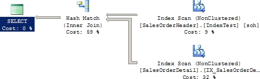
Figure 11-10. Execution plan showing the detrimental effect of using the DATEPART function on a WHERE clause column
This is the output of SET STATISTICS IO and TIME:
Table 'Worktable'. Scan count 0, logical reads 0 Table 'SalesOrderDetail'. Scan count 1, logical reads 273 Table 'SalesOrderHeader'. Scan count 1, logical reads 73 CPU time = 63 ms, elapsed time = 220 ms.
The date part comparison can be done without applying the function on the DATETIME column.
SELECT soh.SalesOrderID,
soh.OrderDate
FROM Sales.SalesOrderHeader AS soh
JOIN Sales.SalesOrderDetail AS sod
ON soh.SalesOrderID = sod.SalesOrderID
WHERE soh.OrderDate >= '2008-04-01'
AND soh.OrderDate < '2008-05-01' ;
This allows the optimizer to properly reference the index IndexTest that was created on the DATETIME column, as shown in Figure 11-11.

Figure 11-11. Execution plan showing the benefit of not using the CONVERT function on a WHERE clause column
This is the output of SETSTATISTICS IO and TIME:
Table 'Worktable'. Scan count 0, logical reads 0
Table 'SalesOrderDetail'. Scan count 1, logical reads 273
Table 'SalesOrderHeader'. Scan count 1, logical reads 8
CPU time = 0 ms, elapsed time = 209 ms
Therefore, to allow the optimizer to consider an index on a column referred to in the WHERE clause, always avoid using a function on the indexed column. This increases the effectiveness of indexes, which can improve query performance. In this instance, though, it’s worth noting that the performance was minor since there’s still a scan of the SalesOrderDetail table.
Be sure to drop the index created earlier.
DROP INDEX Sales.SalesOrderHeader.IndexTest ;
Avoiding Optimizer Hints
SQL Server’s cost-based optimizer dynamically determines the processing strategy for a query based on the current table/index structure and data. This dynamic behavior can be overridden using optimizer hints, taking some of the decisions away from the optimizer by instructing it to use a certain processing strategy. This makes the optimizer behavior static and doesn’t allow it to dynamically update the processing strategy as the table/index structure or data changes.
Since it is usually difficult to outsmart the optimizer, the usual recommendation is to avoid optimizer hints. Generally, it is beneficial to let the optimizer determine a cost-effective processing strategy based on the data distribution statistics, indexes, and other factors. Forcing the optimizer (with hints) to use a specific processing strategy hurts performance more often than not, as shown in the following examples for these hints:
- JOIN hint
- INDEX hint
- FORCEPLAN hint
As explained in Chapter 3, the optimizer dynamically determines a cost-effective JOIN strategy between two data sets based on the table/index structure and data. Table 11-2 presents a summary of the JOIN types supported by SQL Server 2012 for easy reference.
Table 11-2. JOIN Types Supported by SQL Server 2012
|
JOIN Type |
Index on Joining Columns |
Usual Size of Joining Tables |
Presorted JOIN Clause |
|
Nested loop |
Inner table a must. |
Small |
Optional |
|
Outer table preferable. |
|||
|
Merge |
Both tables a must. |
Large |
Yes |
|
Optimal condition: Clustered or covering index on both. |
|||
|
Hash |
Inner table not indexed. |
Any |
No |
|
Optimal condition: Inner table large, outer table small. |
![]() Note The outer table is usually the smaller of the two joining tables.
Note The outer table is usually the smaller of the two joining tables.
You can instruct SQL Server to use a specific JOIN type by using the JOIN hints in Table 11-3.
To understand how the use of JOIN hints can affect performance, consider the following SELECT statement (--joinin the download):
SELECT s.[Name] AS StoreName,
p.[LastName] + ', ' + p.[FirstName]
FROM [Sales].[Store] s
JOIN [Sales].SalesPerson AS sp
ON s.SalesPersonID = sp.BusinessEntityID
JOIN HumanResources.Employee AS e
ON sp.BusinessEntityID = e.BusinessEntityID
JOIN Person.Person AS p
ON e.BusinessEntityID = p.BusinessEntityID ;
Figure 11-12 shows the execution plan.
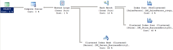
Figure 11-12. Execution plan showing choices made by the optimizer
As you can see, SQL Server dynamically decided to use a LOOP JOIN to add the data from the Person.Person table and to add a HASH JOIN for the Sales.Salesperson and Sales.Store tables. As demonstrated in Chapter 3, for simple queries affecting a small result set, a LOOP JOIN generally provides better performance than a HASH JOIN or MERGE JOIN. Since the number of rows coming from the Sales.Salesperson table is relatively small, it might feel like you could force the JOIN to be a LOOP like this:
SELECT s.[Name] AS StoreName,
p.[LastName] + ', ' + p.[FirstName]
FROM [Sales].[Store] s
JOIN [Sales].SalesPerson AS sp
ON s.SalesPersonID = sp.BusinessEntityID
JOIN HumanResources.Employee AS e
ON sp.BusinessEntityID = e.BusinessEntityID
JOIN Person.Person AS p
ON e.BusinessEntityID = p.BusinessEntityID
OPTION (LOOP JOIN) ;
When this query is run, the execution plan changes, as you can see in Figure 11-13.
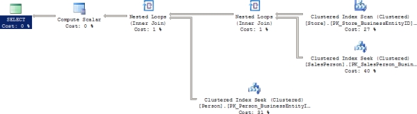
Figure 11-13. Changes made by using the JOIN query hint
Here are the corresponding STATISTICS IO and TIME outputs for each query.
- With no JOIN hint:
Table 'Person'. Scan count 0, logical reads 2155
Table 'Worktable'. Scan count 0, logical reads 0
Table 'Store'. Scan count 1, logical reads 103
Table 'SalesPerson'. Scan count 1, logical reads 2
CPU time = 0 ms, elapsed time = 134 ms.
- With a JOIN hint:
Table 'Person'. Scan count 0, logical reads 2155
Table 'SalesPerson'. Scan count 0, logical reads 1402
Table 'Store'. Scan count 1, logical reads 103
CPU time = 16 ms, elapsed time = 210 ms.
You can see that the query with the JOIN hint takes longer to run than the query without the hint. It also adds overhead to the CPU. And you can make this even worse. Instead of telling all hints used in the query to be a LOOP join, it is possible to target just the one you are interested in, like so:
SELECT s.[Name] AS StoreName,
p.[LastName] + ', ' + p.[FirstName]
FROM [Sales].[Store] s
INNER LOOP JOIN [Sales].SalesPerson AS sp
ON s.SalesPersonID = sp.BusinessEntityID
JOIN HumanResources.Employee AS e
ON sp.BusinessEntityID = e.BusinessEntityID
JOIN Person.Person AS p
ON e.BusinessEntityID = p.BusinessEntityID ;
Running this query results in the execution plan shown in Figure 11-14.
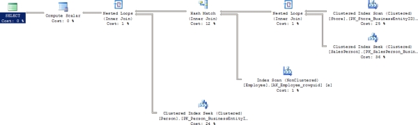
Figure 11-14. More changes from using the LOOP join hint
As you can see, there are now four tables referenced in the query plan. There have been four tables referenced through all the previous executions, but the optimizer was able to eliminate one table from the query through the simplification process of optimization (referred to in Chapter 4). Now the hint has forced the optimizer to make different choices than it otherwise might have and removed simplification from the process. The reads and execution time suffered as well.
Table 'Person'. Scan count 0, logical reads 2155
Table 'Worktable'. Scan count 0, logical reads 0
Table 'Employee'. Scan count 1, logical reads 2
Table 'SalesPerson'. Scan count 0, logical reads 1402
Table 'Store'. Scan count 1, logical reads 103
CPU time = 0 ms, elapsed time = 220 ms.
JOIN hints force the optimizer to ignore its own optimization strategy and use instead the strategy specified by the query. JOIN hints generally hurt query performance because of the following factors:
- Hints prevent autoparameterization.
- The optimizer is prevented from dynamically deciding the joining order of the tables.
Therefore, it makes sense to not use the JOIN hint but to instead let the optimizer dynamically determine a cost-effective processing strategy.
As mentioned earlier, using an arithmetic operator on a WHERE clause column prevents the optimizer
from choosing the index on the column. To improve performance, you can rewrite the query without
using the arithmetic operator on the WHERE clause, as shown in the corresponding example. Alternatively,
you may even think of forcing the optimizer to use the index on the column with an INDEX hint (a type of optimizer hint). However, most of the time, it is better to avoid the INDEX hint and let the optimizer behave dynamically.
To understand the effect of an INDEX hint on query performance, consider the example presented in the “Avoid Arithmetic Operators on the WHERE Clause Column” section. The multiplication operator on the PurchaseOrderID column prevented the optimizer from choosing the index on the column. You can use an INDEX hint to force the optimizer to use the index on the OrderID column as follows:
SELECT *
FROM Purchasing.PurchaseOrderHeader AS poh WITH (INDEX (PK_PurchaseOrderHeader_PurchaseOrderID))
WHERE poh.PurchaseOrderID * 2 = 3400 ;
Note the relative cost of using the INDEX hint in comparison to not using the INDEX hint, as shown in Figure 11-14. Also, note the difference in the number of logical reads shown in the following STATISTICS IO outputs.
- No hint (with the arithmetic operator on the WHERE clause column):
Table 'PurchaseOrderHeader'. Scan count 1, logical reads 11
CPU time = 0 ms, elapsed time = 153 ms.
- No hint (without the arithmetic operator on the WHERE clause column):
Table 'PurchaseOrderHeader'. Scan count 0, logical reads 2
CPU time = 16 ms, elapsed time = 76 ms.
- INDEX hint:
Table 'PurchaseOrderHeader'. Scan count 1, logical reads 44
CPU time = 16 ms, elapsed time = 188 ms.
From the relative cost of execution plans and number of logical reads, it is evident that the query with the INDEX hint actually impaired the query performance. Even though it allowed the optimizer to use the index on the PurchaseOrderID column, it did not allow the optimizer to determine the proper index-access mechanism. Consequently, the optimizer used the index scan to access just one row. In comparison, avoiding the arithmetic operator on the WHERE clause column and not using the INDEX hint allowed the optimizer not only to use the index on the PurchaseOrderID column but also to determine the proper index access mechanism: INDEX SEEK.
Therefore, in general, let the optimizer choose the best indexing strategy for the query, and don’t override the optimizer behavior using an INDEX hint. Also, not using INDEX hints allows the optimizer to decide the best indexing strategy dynamically as the data changes over time.
Using Domain and Referential Integrity
Domain and referential integrity help define and enforce valid values for a column, maintaining the integrity of the database. This is done through column/table constraints.
Since data access is usually one of the most costly operations in a query execution, avoiding redundant data access helps the optimizer reduce the query execution time. Domain and referential integrity help the SQL Server 2012 optimizer analyze valid data values without physically accessing the data, which reduces query time.
To understand how this happens, consider the following examples:
- The NOT NULL constraint
- Declarative referential integrity (DRI)
NOT NULL Constraint
The NOT NULL column constraint is used to implement domain integrity by defining the fact that a NULL value can’t be entered in a particular column. SQL Server automatically enforces this fact at runtime to maintain the domain integrity for that column. Also, defining the NOT NULL column constraint helps the optimizer generate an efficient processing strategy when the ISNULL function is used on that column in a query.
To understand the performance benefit of the NOT NULL column constraint, consider the following example. These two queries are intended to return every value that does not equal ‘B’. These two queries are running against similarly sized columns, each of which will require a table scan in order to return the data (null.sql in the download).
SELECT p.FirstName
FROM Person.Person AS p
WHERE p.FirstName < 'B'
OR p.FirstName >= 'C' ;
SELECT p.MiddleName
FROM Person.Person AS p
WHERE p.MiddleName < 'B'
OR p.MiddleName >= 'C' ;
The two queries use identical execution plans, as you can see in Figure 11-16.
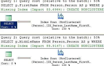
Figure 11-16. Table scans caused by a lack of indexes
Since the column Person.MiddleName can contain NULL, the data returned is incomplete. This is because, by definition, although a NULL value meets the necessary criteria of not being in any way equal to ‘B’, you can’t return NULL values in this manner. An added OR clause is necessary. That would mean modifying the second query like this:
SELECT p.FirstName
FROM Person.Person AS p
WHERE p.FirstName < 'B'
OR p.FirstName >= 'C' ;
SELECT p.MiddleName
FROM Person.Person AS p
WHERE p.MiddleName < 'B'
OR p.MiddleName >= 'C'
OR p.MiddleName IS NULL ;
Also, as shown in the missing index statements in the execution plan in Figure 11-15, these two queries can benefit from having indexes created on their tables. Creating test indexes like the following should satisfy the requirements:
CREATE INDEX TestIndex1
ON Person.Person (MiddleName) ;
CREATE INDEX TestIndex2
ON Person.Person (FirstName) ;
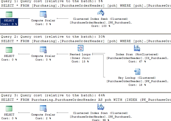
Figure 11-15. Cost of a query with and without different INDEX hints
When the queries are reexecuted, Figure 11-17 shows the resultant execution plan for the two SELECT statements.
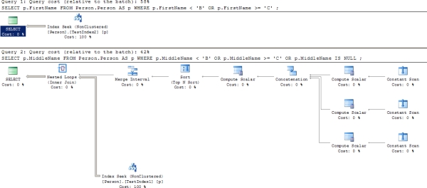
Figure 11-17. Effect of the IS NULL option being used
As shown in Figure 11-17, the optimizer was able to take advantage of the index TestIndex2 on the Person.FirstName column to get a nice clean Index Seek operation. Unfortunately, the requirements for processing the NULL columns were very different. The index TestIndex1 was not used in the same way. Instead, three constants were created for each of the three criteria defined within the query. These were then joined together through the Concatenation operation, sorted and merged prior to scanning the index three times through the Nested Loop operator to arrive at the result set. Although it appears, from the estimated costs in the execution plan, that this was the less costly query (42 percent compared to 58 percent), STATISTICS 10 and TIME tell the more accurate story, which is that the NULL queries were more costly.
Table 'Person'. Scan count 2, logical reads 66 CPU time = 0 ms, elapsed time = 257 ms.
vs.
Table 'Person'. Scan count 3, logical reads 42 CPU time = 0 ms, elapsed time = 397 ms.
Be sure to drop the test indexes that were created.
DROP INDEX TestIndex1 ON Person.Person ;
DROP INDEX TestIndex2 ON Person.Person ;
As much as possible, you should attempt to leave NULL values out of the database. However, when data is unknown, default values may not be possible. That’s when NULL will come back into the design. I find NULLs to be unavoidable, but they are something to minimize as much as you can.
When it is unavoidable and you will be dealing with NULL values, keep in mind that you can use a filtered index that removes NULL values from the index, thereby improving the performance of that index. This was detailed in Chapter 4. Sparse columns offer another option to help you deal with NULL values. Sparse columns are primarily aimed at storing NULL values more efficiently and therefore reduce space—at a sacrifice in performance. This option is specifically targeted at business intelligence (BI) databases, not OLTP databases where large amounts of NULL values in fact tables are a normal part of the design.
Declarative Referential Integrity
Declarative referential integrity is used to define referential integrity between a parent table and a child table. It ensures that a record in the child table exists only if the corresponding record in the parent table exists. The only exception to this rule is that the child table can contain a NULL value for the identifier that links the rows of the child table to the rows of the parent table. For all other values of the identifier in the child, a corresponding value must exist in the parent table. In SQL Server, DRI is implemented using a PRIMARY KEY constraint on the parent table and a FOREIGN KEY constraint on the child table.
With DRI established between two tables and the foreign key columns of the child table set to NOT NULL, the SQL Server 2012 optimizer is assured that for every record in the child table, the parent table has a corresponding record. Sometimes this can help the optimizer improve performance, because accessing the parent table is not necessary to verify the existence of a parent record for a corresponding child record.
To understand the performance benefit of implementing declarative referential integrity, let’s consider an example. First, eliminate the referential integrity between two tables, Person.Address and Person.StateProvince, using this script:
IF EXISTS ( SELECT *
FROM sys.foreign_keys
WHERE object_id = OBJECT_ID(N'[Person].[FK_Address_StateProvince_StateProvinceID]')
AND parent_object_id = OBJECT_ID(N'[Person].[Address]') )
ALTER TABLE [Person].[Address] DROP CONSTRAINT [FK_Address_StateProvince_StateProvinceID] ;
Consider the following SELECT statement (--prod in the download):
SELECT a.AddressID,
sp.StateProvinceID
FROM Person.Address AS a
JOIN Person.StateProvince AS sp
ON a.StateProvinceID = sp.StateProvinceID
WHERE a.AddressID = 27234 ;
Note that the SELECT statement fetches the value of the StateProvinceID column from the parent table (Person.Address). If the nature of the data requires that for every product (identified by StateProvinceId) in the child table (Person.StateProvince) the parent table (Person.Address) contains a corresponding product, then you can rewrite the preceding SELECT statement as follows (--prod2 in the download):
SELECT a.AddressID,
a.StateProvinceID
FROM Person.Address AS a
JOIN Person.StateProvince AS sp
ON a.StateProvinceID = sp.StateProvinceID
WHERE a.AddressID = 27234 ;
Both SELECT statements should return the same result set. Even the optimizer generates the same execution plan for both the SELECT statements, as shown in Figure 11-18.
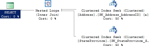
Figure 11-18. Execution plan when DRI is not defined between the two tables
To understand how declarative referential integrity can affect query performance, replace the FOREIGN KEY dropped earlier.
ALTER TABLE [Person].[Address]
WITH CHECK ADD CONSTRAINT [FK_Address_StateProvince_StateProvinceID]
FOREIGN KEY ([StateProvinceID])
REFERENCES [Person].[StateProvince] ([StateProvinceID]) ;
![]() Note There is now referential integrity between the tables.
Note There is now referential integrity between the tables.
Figure 11-19 shows the resultant execution plans for the two SELECT statements.
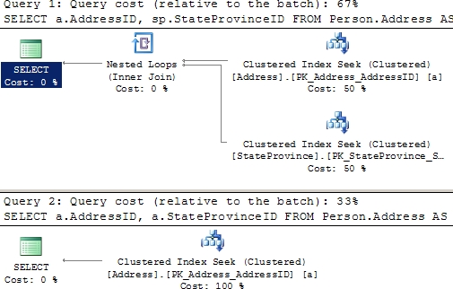
Figure 11-19. Execution plans showing the benefit of defining DRI between the two tables
As you can see, the execution plan of the second SELECT statement is highly optimized: the Person.StateProvince table is not accessed. With the declarative referential integrity in place (and Address.StateProvince set to NOT NULL), the optimizer is assured that for every record in the child table, the parent table contains a corresponding record. Therefore, the JOIN clause between the parent and child tables is redundant in the second SELECT statement, with no other data requested from the parent table.
You probably already knew that domain and referential integrity are Good Things, but you can see that they not only ensure data integrity but also improve performance. As just illustrated, domain and referential integrity provide more choices to the optimizer to generate cost-effective execution plans and improve performance.
To achieve the performance benefit of DRI, as mentioned previously, the foreign key columns in the child table should be NOT NULL. Otherwise, there can be rows (with foreign key column values as NULL) in the child table with no representation in the parent table. That won’t prevent the optimizer from accessing the primary table (Prod) in the previous query. By default—that is, if the NOT NULL attribute isn’t mentioned for a column—the column can have NULL values. Considering the benefit of the NOT NULL attribute and the other benefits explained in this section, always mark the attribute of a column as NOT NULL if NULL isn’t a valid value for that column.
You also must make sure that you are using the WITH CHECK option when building your foreign key constraints. If the NOCHECK option is used, these are considered to be untrustworthy constraints by the optimizer and you won’t realize the performance benefits that they can offer.
Avoiding Resource-Intensive Queries
Many database functionalities can be implemented using a variety of query techniques. The approach you should take is to use query techniques that are very resource friendly and set-based. A few techniques you can use to reduce the footprint of a query are as follows:
- Avoid data type conversion.
- Use EXISTS over COUNT(*) to verify data existence.
- Use UNION ALL over UNION.
- Use indexes for aggregate and sort operations.
- Avoid local variables in a batch query.
- Be careful naming stored procedures.
I cover these points in more detail in the next sections.
Avoid Data Type Conversion
SQL Server allows, in some instances (defined by the large table of data conversions available in Books Online), a value/constant with different but compatible data types to be compared with a column’s data. SQL Server automatically converts the data from one data type to another. This process is called implicit data type conversion. Although useful, implicit conversion adds overhead to the query optimizer. To improve performance, use a variable/constant with the same data type as that of the column to which it is compared.
To understand how implicit data type conversion affects performance, consider the following example (--conversion in the download):
IF EXISTS ( SELECT *
FROM sys.objects
WHERE object_id = OBJECT_ID(N'dbo.Test1') )
DROP TABLE dbo.Test1 ;
CREATE TABLE dbo.Test1
(Id INT IDENTITY(1, 1),
MyKey VARCHAR(50),
MyValue VARCHAR(50)
) ;
CREATE UNIQUE CLUSTERED INDEX Test1PrimaryKey ON dbo.Test1 ([Id] ASC) ;
CREATE UNIQUE NONCLUSTERED INDEX TestIndex ON dbo.Test1 (MyKey) ;
GO
SELECT TOP 10000
IDENTITY( INT,1,1 ) AS n
INTO #Tally
FROM Master.dbo.SysColumns scl,
Master.dbo.SysColumns sc2 ;
INSERT INTO dbo.Test1
(MyKey,
MyValue
)
SELECT TOP 10000
'UniqueKey' + CAST(n AS VARCHAR),
'Description'
FROM #Tally ;
DROP TABLE #Tally ;
SELECT t.MyValue
FROM dbo.Test1 AS t
WHERE t.MyKey = 'UniqueKey333' ;
SELECT t.MyValue
FROM dbo.Test1 AS t
WHERE t.MyKey = N'UniqueKey333' ;
After creating the table Test1, creating a couple of indexes on it, and placing some data, two queries are defined. Both queries return the same result set. As you can see, both queries are identical except for the data type of the variable equated to the MyKey column. Since this column is VARCHAR, the first query doesn’t require an implicit data type conversion. The second query uses a different data type from that of the MyKey column, requiring an implicit data type conversion and thereby adding overhead to the query performance. Figure 11-20 shows the execution plans for both queries.
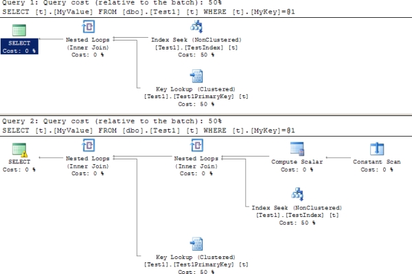
Figure 11-20. Cost of a query with and without implicit data type conversion
The complexity of the implicit data type conversion depends on the precedence of the data types involved in the comparison. The data type precedence rules of SQL Server specify which data type is converted to the other. Usually, the data type of lower precedence is converted to the data type of higher precedence. For example, the TINYINT data type has a lower precedence than the INT data type. For a complete list of data type precedence in SQL Server 2012, please refer to the MSDN article “Data Type Precedence” (http://msdn.microsoft.com/en-us/library/ms190309.aspx). For further information about which data type can implicitly convert to which data type, refer to the MSDN article “Data Type Conversion” (http://msdn.microsoft.com/en-us/library/ms191530.aspx).
Note the warning icon on the SELECT operator. It’s letting you know that there’s something questionable in this query. In this case, it’s the fact that there is a data type conversion operation. The optimizer lets you know that this might negatively affect its ability to find and use an index to assist the performance of the query.
When SQL Server compares a column value with a certain data type and a variable (or constant) with a different data type, the data type of the variable (or constant) is always converted to the data type of the column. This is done because the column value is accessed based on the implicit conversion value of the variable (or constant). Therefore, in such cases, the implicit conversion is always applied on the variable (or constant).
As you can see, implicit data type conversion adds overhead to the query performance both in terms of a poor execution plan and in added CPU cost to make the conversions. Therefore, to improve performance, always use the same data type for both expressions.
Use EXISTS over COUNT(*) to Verify Data Existence
A common database requirement is to verify whether a set of data exists. Usually you’ll see this implemented using a batch of SQL queries, as follows (--count in the download):
DECLARE @n INT ;
SELECT @n = COUNT(*)
FROM Sales.SalesOrderDetail AS sod
WHERE sod.OrderQty = 1 ;
IF @n > 0
PRINT 'Record Exists' ;
Using COUNT(*)to verify the existence of data is highly resource-intensive, because COUNT(*) has to scan all the rows in a table. EXISTS merely has to scan and stop at the first record that matches the EXISTS criterion. To improve performance, use EXISTS instead of the COUNT(*) approach.
IF EXISTS ( SELECT sod.*
FROM Sales.SalesOrderDetail AS sod
WHERE sod.OrderQty = 1 )
PRINT 'Record Exists';
The performance benefit of the EXISTS technique over the COUNT(*) technique can be compared using the STATISTICS IO and TIME output, as well as the execution plan in Figure 11-21, as you can see from the output of running these queries.
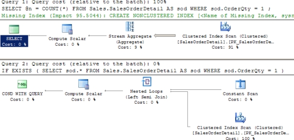
Figure 11-21. Difference between COUNT and EXISTS
Table 'SalesOrderDetail'. Scan count 1, logical reads 1240
CPU time = 31 ms, elapsed time = 30 ms.
Table 'SalesOrderDetail'. Scan count 1, logical reads 3
CPU time = 0 ms, elapsed time = 12 ms.
As you can see, the EXISTS technique used only three logical reads compared to the 1,240 used by the COUNT(*) technique, and the execution time went from 30 ms to 12. Therefore, to determine whether data exists, use the EXISTS technique.
Use UNION ALL Instead of UNION
You can concatenate the result set of multiple SELECT statements using the UNION clause as follows:
SELECT *
FROM Sales.SalesOrderHeader AS soh
WHERE soh.SalesOrderNumber LIKE '%47808'
UNION
SELECT *
FROM Sales.SalesOrderHeader AS soh
WHERE soh.SalesOrderNumber LIKE '%65748' ;
The UNION clause processes the result set from the two SELECT statements, removing duplicates from the final result set and effectively running DISTINCT on each query. If the result sets of the SELECT statements participating in the UNION clause are exclusive to each other or you are allowed to have duplicate rows in the final result set, then use UNION ALL instead of UNION. This avoids the overhead of detecting and removing any duplicates, improving performance, as shown in Figure 11-23.
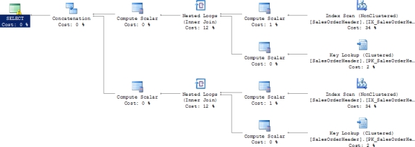
Figure 11-23. The execution plan of the query using UNION ALL
As you can see, in the first case (using UNION), the optimizer used a unique sort to process the duplicates while concatenating the result set of the two SELECT statements. Since the result sets are exclusive to each other, you can use UNION ALL instead of the UNION clause. Using the UNION ALL clause avoids the overhead of detecting duplicates and thereby improves performance.
Use Indexes for Aggregate and Sort Conditions
Generally, aggregate functions such as MIN and MAX benefit from indexes on the corresponding column. Without any index on the column, the optimizer has to scan the base table (or the clustered index), retrieve all the rows, and perform a stream aggregate on the group (containing all rows) to identify the MIN/MAX value, as shown in the following example:
SELECT MIN(sod.UnitPrice)
FROM Sales.SalesOrderDetail AS sod ;
The STATISTICS IO and TIME output of the SELECT statement using the MIN aggregate function is as follows:
Table 'SalesOrderDetail'. Scan count 1, logical reads 1240 CPU time = 47 ms, elapsed time = 44 ms.
As shown in the STATISTICS output, the query performed more than 1,000 logical reads just to retrieve the row containing the minimum value for the UnitPrice column. If you create an index on the UnitPrice column, then the UnitPrice values will be presorted by the index in the leaf pages.
CREATE INDEX TestIndex ON Sales.SalesOrderDetail (UnitPrice ASC) ;
The index on the UnitPrice column improves the performance of the MIN aggregate function significantly. The optimizer can retrieve the minimum UnitPrice value by seeking to the topmost row in the index. This reduces the number of logical reads for the query, as shown in the corresponding STATISTICS output.
Table 'SalesOrderDetail'. Scan count 1, logical reads 3 CPU time = 0 ms, elapsed time = 0 ms.
Similarly, creating an index on the columns referred to in an ORDER BY clause helps the optimizer organize the result set fast because the column values are prearranged in the index. The internal implementation of the GROUP BY clause also sorts the column values first because sorted column values allow the adjacent matching values to be grouped quickly. Therefore, like the ORDER BY clause, the GROUP BY clause also benefits from having the values of the columns referred to in the GROUP BY clause sorted in advance.
Avoid Local Variables in a Batch Query
Often, multiple queries are submitted together as a batch, avoiding multiple network round-trips. It’s common to use local variables in a query batch to pass a value between the individual queries. However, using local variables in the WHERE clause of a query in a batch doesn’t allow the optimizer to generate an efficient execution plan.
To understand how the use of a local variable in the WHERE clause of a query in a batch can affect performance, consider the following batch query (--batch):
DECLARE @id INT = 1 ;
SELECT pod.*
FROM Purchasing.PurchaseOrderDetail AS pod
JOIN Purchasing.PurchaseOrderHeader AS poh
ON poh.PurchaseOrderID = pod.PurchaseOrderID
WHERE poh.PurchaseOrderID >= @id ;
Figure 11-24 shows the execution plan of this SELECT statement.

Figure 11-24. Execution plan showing the effect of a local variable in a batch query
As you can see, an Index Seek operation is performed to access the rows from the Purchasing.PurchaseOrderDetail table. If the SELECT statement is executed without using the local variable, by replacing the local variable value with an appropriate constant value as in the following query, the optimizer makes different choices.
SELECT pod.*
FROM Purchasing.PurchaseOrderDetail AS pod
JOIN Purchasing.PurchaseOrderHeader AS poh
ON poh.PurchaseOrderID = pod.PurchaseOrderID
WHERE poh.PurchaseOrderID >= 1 ;
Figure 11-25 shows the result.
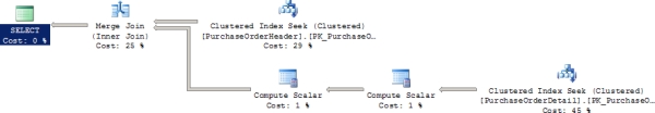
Figure 11-25. Execution plan for the query when the local variable is not used
Although these two approaches look identical, on closer examination, interesting differences begin to appear. Notice the estimated cost of some of the operations. For example, the Merge Join is different between Figure 11-22 and Figure 11-23; it’s 29 percent in the first and 25 percent in the second. If you look at STATISTICS IO and TIME for each query, other differences appear. First, here’s the information from the initial query:
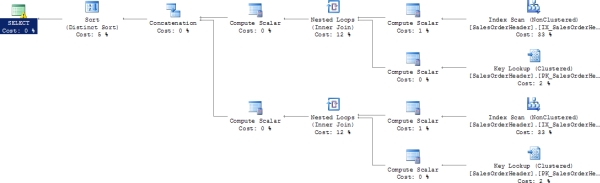
Figure 11-22. The execution plan of the query using the UNION clause
Table 'PurchaseOrderDetail'. Scan count 1, logical reads 66
Table 'PurchaseOrderHeader'. Scan count 1, logical reads 44
CPU time = 0 ms, elapsed time = 505 ms.
Then here's the second query, without the local variable:
Table 'PurchaseOrderDetail'. Scan count 1, logical reads 66
Table 'PurchaseOrderHeader'. Scan count 1, logical reads 44
CPU time = 46 ms, elapsed time = 441 ms.
Notice that the scans and reads are the same, as might be expected of queries with near identical plans. The CPU and elapsed times are different, with the second query (the one without the local variable) consistently being a little less. Based on these facts, you may assume that the execution plan of the first query will be somewhat more costly compared to the second query. But the reality is quite different, as shown in the execution plan cost comparison in Figure 11-26.
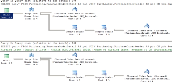
Figure 11-26. Relative cost of the query with and without the use of a local variable
From the relative cost of the two execution plans, it appears that the second query isn’t cheaper than the first query. However, from the STATISTICS comparison, it appears that the second query should be cheaper than the first query. Which one should you believe: the comparison of STATISTICS or the relative cost of the execution plan? What’s the source of this anomaly?
The execution plan is generated based on the optimizer’s estimation of the number of rows affected for each execution step. If you take a look at the properties for the various operators in the initial execution plan for
the query with the local variable (as shown in Figure 11-24), you may notice a disparity. Take a look at this in
Figure 11-27.
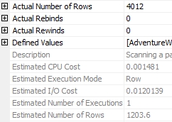
Figure 11-27. Clustered index seek details with a local variable
The disparity you’re looking for is the Actual Number of Rows value (at the top) compared to the Estimated Number of Rows value (at the bottom). In the properties shown in Figure 11-27, there are 1203.6 estimated rows, while the actual number is considerably higher at 4012. If you compare this to the same operator in the second query (the one without the local variable), you may notice something else. Take a look at Figure 11-28.
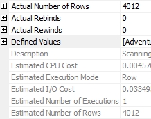
Figure 11-28. Clustered index seek details without a local variable
Here you’ll see that the Actual Number of Rows and Estimated Number of Rows values are the same: 4012. From these two measures, you can see that the estimated rows for the execution steps of the first query (using a local variable in the WHERE clause) is way off the actual number of rows returned by the steps. Consequently, the execution plan cost for the first query, which is based on the estimated rows, is somewhat misleading. The incorrect estimation misguides the optimizer and somewhat causes some variations in how the query is executed. You can see this in the return times on the query, even though the number of rows returned is identical.
Any time you find such an anomaly between the relative execution plan cost and the STATISTICS output for the queries under analysis, you should verify the basis of the estimation. If the underlying facts (estimated rows) of the execution plan itself are wrong, then it is quite likely that the cost represented in the execution plan will also be wrong. But since the output of the various STATISTICS measurements shows the actual number of logical reads and the real elapsed time required to perform the query without being affected by the initial estimation, you can rely on the STATISTICS output.
Now let’s return to the actual performance issue associated with using local variables in the WHERE clause. As shown in the preceding example, using the local variable as the filter criterion in the WHERE clause of a batch query doesn’t allow the optimizer to determine the right indexing strategy. This happens because, during the optimization of the queries in the batch, the optimizer doesn’t know the value of the variable used in the WHERE clause and can’t determine the right access strategy—it knows the value of the variable only during execution. You can further see this by noting that the second query in Figure 11-24 has a missing index alert, suggesting a possible way to improve the performance of the query, whereas the query with the local variable is unable to make that determination.
To avoid this particular performance problem, use one of the following approaches:
- Don’t use a local variable as a filter criterion in a batch for a query like this. A local variable is different than a parameter value, as I’ll demonstrate in a minute.
- Create a stored procedure for the batch, and execute it as follows (--batchproc):
CREATE PROCEDURE spProductDetails (@id INT)
AS
SELECT pod.*
FROM Purchasing.PurchaseOrderDetail AS pod
JOIN Purchasing.PurchaseOrderHeader AS poh
ON poh.PurchaseOrderID = pod.PurchaseOrderID
WHERE poh.PurchaseOrderID >= @id ;
GO
EXEC spProductDetails
@id = 1 ;
The optimizer generates the same execution plan as the query that doesn’t use a local variable for the ideal case. Correspondingly, the execution time is also reduced. In the case of a stored procedure, the optimizer generates the execution plan during the first execution of the stored procedure and uses the parameter value supplied to determine the right processing strategy.
This approach can backfire. The process of using the values passed to a parameter is referred to as parameter sniffing. Parameter sniffing occurs for all stored procedures and parameterized queries automatically. Depending on the accuracy of the statistics and the values passed to the parameters, it is possible to get a bad plan using specific values and a good plan using the sampled values that occur when you have a local variable. Testing is the only way to be sure which will work best in any given situation. However, in most circumstances, you’re better off having accurate values rather than sampled ones.
Be Careful When Naming Stored Procedures
The name of a stored procedure does matter. You should not name your procedures with a prefix of sp_. Developers often prefix their stored procedures with sp_ so that they can easily identify the stored procedures. However, SQL Server assumes that any stored procedure with this exact prefix is probably a system stored procedure, whose home is in the master database. When a stored procedure with an sp_ prefix is submitted for execution, SQL Server looks for the stored procedure in the following places in the following order:
- In the master database
- In the current database based on any qualifiers provided (database name or owner)
- In the current database using dbo as the schema, if a schema is not specified
Therefore, although the user-created stored procedure prefixed with sp_ exists in the current database, the master database is checked first. This happens even when the stored procedure is qualified with the database name.
To understand the effect of prefixing sp_ to a stored procedure name, consider the following stored procedure (--spDont in the download):
IF EXISTS ( SELECT *
FROM sys.objects
WHERE object_id = OBJECT_ID(N'[dbo].[sp_Dont]')
AND type IN (N'P', N'PC') )
DROP PROCEDURE [dbo].[sp_Dont]
GO
CREATE PROC [sp_Dont]
AS
PRINT 'Done!'
GO
--Add plan of sp_Dont to procedure cache
EXEC AdventureWorks2008R2.dbo.[sp_Dont] ;
GO
--Use the above cached plan of sp_Dont
EXEC AdventureWorks2008R2.dbo.[sp_Dont] ;
GO
The first execution of the stored procedure adds the execution plan of the stored procedure to the procedure cache. A subsequent execution of the stored procedure reuses the existing plan from the procedure cache unless a recompilation of the plan is required (the causes of stored procedure recompilation are explained in Chapter 10). Therefore, the second execution of the stored procedure spDont shown in Figure 11-29 should find a plan in the procedure cache. This is indicated by an SP:CacheHit event in the corresponding Extended Event output.
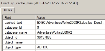
Figure 11-29. Extended Events output showing the effect of the sp_ prefix on a stored procedure name
Note that an SP:CacheMiss event is fired before SQL Server tries to locate the plan for the stored procedure in the procedure cache. The SP:CacheMiss event is caused by SQL Server looking in the master database for the stored procedure, even though the execution of the stored procedure is properly qualified with the user database name.
This aspect of the sp_ prefix becomes more interesting when you create a stored procedure with the name of an existing system stored procedure (--spaddmessage in the download).
CREATE PROC sp_addmessage @param1 NVARCHAR(25)
AS
PRINT '@param1 = ' + @param1 ;
GO
EXEC AdventureWorks2008R2.dbo.[sp_addmessage] 'AdventureWorks';
The execution of this user-defined stored procedure causes the execution of the system stored procedure sp_addmessage from the master database instead, as you can see in Figure 11-30.
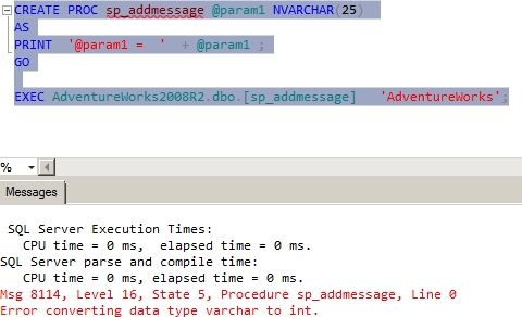
Figure 11-30. Execution result for stored procedure showing the effect of the sp_ prefix on a stored procedure name
Unfortunately, it is not possible to execute this user-defined stored procedure.
![]() Tip As a side note, please don’t try to execute the DROP PROCEDURE statement on this stored procedure twice. On the second execution, the system stored procedure will be dropped from the master database.
Tip As a side note, please don’t try to execute the DROP PROCEDURE statement on this stored procedure twice. On the second execution, the system stored procedure will be dropped from the master database.
You can see now why you should not prefix a user-defined stored procedure’s name with sp_. Use some other naming convention.
Reducing the Number of Network Round-Trips
Database applications often execute multiple queries to implement a database operation. Besides optimizing the performance of the individual query, it is important that you optimize the performance of the batch. To reduce the overhead of multiple network round-trips, consider the following techniques:
- Execute multiple queries together.
- Use SET NOCOUNT.
Let’s look at these techniques in a little more depth.
Execute Multiple Queries Together
It is preferable to submit all the queries of a set together as a batch or a stored procedure. Besides reducing the network round-trips between the database application and the server, stored procedures also provide multiple performance and administrative benefits, as described in Chapter 9. This means that the code in the application needs to be able to deal with multiple result sets. It also means your T-SQL code may need to deal with XML data or other large sets of data, not single-row inserts or updates.
You need to consider one more factor when executing a batch or a stored procedure. After every query in the batch or the stored procedure is executed, the server reports the number of rows affected.
(<Number> row(s) affected)
This information is returned to the database application and adds to the network overhead. Use the T-SQL statement SET NOCOUNT to avoid this overhead.
SET NOCOUNT ON <SQL queries> SET NOCOUNT OFF
Note that the SET NOCOUNT statement doesn’t cause any recompilation issue with stored procedures, unlike some SET statements, as explained in Chapter 10.
Reducing the Transaction Cost
Every action query in SQL Server is performed as an atomic action so that the state of a database table moves from one consistent state to another. SQL Server does this automatically and it can’t be disabled. If the transition from one consistent state to another requires multiple database queries, then atomicity across the multiple queries should be maintained using explicitly defined database transactions. The old and new state of every atomic action is maintained in the transaction log (on the disk) to ensure durability, which guarantees that the outcome of an atomic action won’t be lost once it completes successfully. An atomic action during its execution is isolated from other database actions using database locks.
Based on the characteristics of a transaction, here are two broad recommendations to reduce the cost of the transaction:
- Reduce logging overhead.
- Reduce lock overhead.
Reduce Logging Overhead
A database query may consist of multiple data manipulation queries. If atomicity is maintained for each query separately, then a large number of disk writes are performed on the transaction log. Since disk activity is extremely slow compared to memory or CPU activity, the excessive disk activity can increase the execution time of the database functionality. For example, consider the following batch query (--logging in the download):
--Create a test table
IF (SELECT OBJECT_ID('dbo.Test1')
) IS NOT NULL
DROP TABLE dbo.Test1 ;
GO
CREATE TABLE dbo.Test1 (C1 TINYINT) ;
GO
--Insert 10000 rows
DECLARE @Count INT = 1 ;
WHILE @Count <= 10000
BEGIN
INSERT INTO dbo.Test1
(C1)
VALUES (@Count % 256) ;
SET @Count = @Count + 1 ;
END
Since every execution of the INSERT statement is atomic in itself, SQL Server will write to the transaction log for every execution of the INSERT statement.
An easy way to reduce the number of log disk writes is to include the action queries within an explicit transaction.
BEGIN TRANSACTION
WHILE @Count <= 10000
BEGIN
INSERT INTO t1
VALUES (@Count % 256) ;
SET @Count = @Count + 1 ;
END
COMMIT
The defined transaction scope (between the BEGIN TRANSACTION and COMMIT pair of commands) expands the scope of atomicity to the multiple INSERT statements included within the transaction. This decreases the number of log disk writes and improves the performance of the database functionality. To test this theory, run the following T-SQL command before and after each of the WHILE loops:
This will show you the percentage of log space used. On running the first set of inserts on my database, the log went from 2.6 percent used to 29 percent. When running the second set of inserts, the log grew about 6 percent.
The best way is to work with sets of data rather than individual rows. A WHILE loop can be an inherently costly operation, like a cursor (more details on cursors in Chapter 14). So, running a query that avoids the WHILE loop and instead works from a set-based approach is even better.
DECLARE @Count INT = 1 ;
BEGIN TRANSACTION
WHILE @Count <= 10000
BEGIN
INSERT INTO dbo.Test1
(C1)
VALUES (@Count % 256) ;
SET @Count = @Count + 1 ;
END
COMMIT
Running this query with the DBCC SQLPERF() function before and after showed less than 4 percent growth of the used space within the log, and it ran in 41 ms as compared to more than 2 seconds for the WHILE loop.
One area of caution, however, is that by including too many data manipulation queries within a transaction, the duration of the transaction is increased. During that time, all other queries trying to access the resources referred to in the transaction are blocked.
Reduce Lock Overhead
By default, all four SQL statements (SELECT, INSERT, UPDATE, and DELETE) use database locks to isolate their work from that of other SQL statements. This lock management adds a performance overhead to the query. The performance of a query can be improved by requesting fewer locks. By extension, the performance of other queries are also improved because they have to wait a shorter period of time to obtain their own locks.
By default, SQL Server can provide row-level locks. For a query working on a large number of rows, requesting a row lock on all the individual rows adds a significant overhead to the lock-management process. You can reduce this lock overhead by decreasing the lock granularity, say to the page level or table level. SQL Server performs the lock escalation dynamically by taking into consideration the lock overheads. Therefore, generally, it is not necessary to manually escalate the lock level. But, if required, you can control the concurrency of a query programmatically using lock hints as follows:
SELECT * FROM <TableName> WITH(PAGLOCK) --Use page level lock
Similarly, by default, SQL Server uses locks for SELECT statements besides those for INSERT, UPDATE, and DELETE statements. This allows the SELECT statements to read data that isn’t being modified. In some cases, the data may be quite static, and it doesn’t go through much modification. In such cases, you can reduce the lock overhead of the SELECT statements in one of the following ways:
- Mark the database as READONLY.
ALTER DATABASE <DatabaseName> SET READONLY
This allows users to retrieve data from the database, but it prevents them from modifying the data. The setting takes effect immediately. If occasional modifications to the database are required, then it may be temporarily converted to READWRITE mode.
ALTER DATABASE <DatabaseName> SET READ_WRITE
<Database modifications>
ALTER DATABASE <DatabaseName> SET READONLY
- Place the specific tables on a filegroup, and mark the filegroup as READONLY.
--Add a new filegroup with a file to the database.
ALTER DATABASE AdventureWorks2008R2
ADD FILEGROUP READONLYFILEGROUP ;
GO
ALTER DATABASE AdventureWorks2008R2
ADD FILE(NAME=ReadOnlyFile, FILENAME='C:Dataadw_l.ndf')
TO FILEGROUP READONLYFILEGROUP ;
GO
--Create specific table(s) on the new filegroup.
CREATE TABLE Tl (Cl INT, C2 INT)
ON READONLYFILEGROUP ;
CREATE CLUSTERED INDEX II ON Tl(Cl);
INSERT INTO Tl
VALUES (1, 1);
--Or move existing table(s) to the new filegroup
CREATE CLUSTERED INDEX II ON Tl(Cl)
WITH DROP_EXISTING ON READONLYFILEGROUP ;
--Set the filegroup property to READONLY.
ALTER DATABASE AdventureWorks2008R2
MODIFY FILEGROUP READONLYFILEGROUP READONLY
This allows you to limit the data access to only the tables residing on the specific file-group to READONLY but keep the data access to tables on other filegroups as READWRITE. This filegroup setting takes effect immediately. If occasional modifications to the specific tables are required, then the property of the corresponding filegroup may be temporarily converted to READWRITE mode.
ALTER DATABASE AdventureWorks2008R2
MODIFY FILEGROUP READONLYFILEGROUP READWRITE <Database modifications> ALTER DATABASE AdventureWorks2008
MODIFY FILEGROUP READONLYFILEGROUP READONLY
- Use one of the snapshot isolations.
SQL Server provides a mechanism to put versions of data into tempdb as updates are occurring, radically reducing locking overhead and blocking for read operations. You can change the isolation level of the database by using an ALTER statement.
ALTER DATABASE AdventureWorks2008R2 SET TRANSACTION ISOLATION LEVEL READ_COMMITTED_SNAPSHOT;
- Prevent SELECT statements from requesting any lock.
SELECT * FROM <TableName> WITH(NOLOCK)
This prevents the SELECT statement from requesting any lock, and it is applicable to SELECT statements only. Although the NOLOCK hint can’t be used directly on the tables referred to in the action queries (INSERT, UPDATE, and DELETE), it may be used on the data-retrieval part of the action queries, as shown here:
DELETE Sales.SalesOrderDetail
FROM Sales.SalesOrderDetail sod WITH(NOLOCK)
JOIN Production.Product p WITH(NOLOCK)
ON sod.ProductID = p.ProductID
AND p.ProductID = 0
Just know that this leads to dirty reads, which can cause duplicate rows or missing rows and is therefore considered to be a last resort to control locking. The best approach is to mark the database as read-only or use one of the snapshot isolation levels.
This is a huge topic and a lot more can be said about it. I discuss the different types of lock requests and how to manage lock overhead in the next chapter. If you made any of the proposed changes to the database from this section, I would recommend restoring from a backup.
Summary
As discussed in this chapter, to improve the performance of a database application, it is important to ensure that SQL queries are designed properly to benefit from performance-enhancement techniques such as indexes, stored procedures, database constraints, and so on. Ensure that queries are resource friendly and don’t prevent the use of indexes. In many cases the optimizer has the ability to generate cost-effective execution plans irrespective of query structure, but it is still a good practice to design the queries properly in the first place. Even after you design individual queries for great performance, the overall performance of a database application may not be satisfactory. It is important not only to improve the performance of individual queries but also to ensure that they work well with other queries without causing serious blocking issues. In the next chapter, you will look into the different blocking aspects of a database application.