Chapter 4
![]()
The right index on the right column, or columns, is the basis on which query tuning begins. On the other hand, a missing index or an index placed on the wrong column, or columns, can be the basis for all performance problems starting with basic data access, continuing through joins, and ending in filtering clauses. For these reasons, it is extremely important for everyone—not just the DBA—to understand the different indexing techniques that can be used to optimize the database design.
In this chapter, I cover the following topics:
- What an index is
- The benefits and overhead of an index
- General recommendations for index design
- Clustered and nonclustered index behavior and comparisons
- Recommendations for clustered and nonclustered indexes
- Advanced indexing techniques: covering indexes, index intersections, index joins, filtered indexes, distributed indexes, indexed views, index compression, and columnstore indexes
- Special index types
- Additional characteristics of indexes
What Is an Index?
One of the best ways to reduce disk I/O is to use an index. An index allows SQL Server to find data in a table without scanning the entire table. An index in a database is analogous to an index in a book. Say, for example, that you wanted to look up the phrase table scan in this book. In the paper version, without the index at the back of the book, you would have to peruse the entire book to find the text you needed. With the index, you know exactly where the information you want is stored.
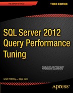
While tuning a database for performance, you create indexes on the different columns used in a query to help SQL Server find data quickly. For example, the following query against the Production.Product table results in the data shown in Figure 4-1 (the first 10 of 500+ rows).
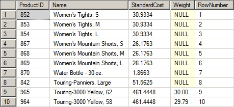
Figure 4-1. Sample Production.Product table
SELECT TOP 10
p.ProductID,
p.[Name],
p.StandardCost,
p.[Weight],
ROW_NUMBER() OVER (ORDER BY p.Name DESC) AS RowNumber
FROM Production.Product p ;
The preceding query scanned the entire table since there was no WHERE clause. If you need to add a filter through the WHERE clause to retrieve all the products where StandardCost is greater than 150, without an index the table will still have to be scanned, checking the value of StandardCost at each row to determine which rows contain a value greater than 150. An index on the StandardCost column could speed up this process by providing a mechanism that allows a structured search against the data rather than a row-by-row check. You can take two different, and fundamental, approaches for creating this index:
- Like a dictionary: A dictionary is a distinct listing of words in alphabetical order. An index can be stored in a similar fashion. The data is ordered, although it will still have duplicates. The first ten rows, ordered by StandardCost instead of by Name, would look like the data shown in Figure 4-2. Notice the RowNumber column shows the original placement of the row when ordering by Name.
Figure 4-2. Product table sorted on StandardCost
So now if you wanted to find all the rows where StandardCost is greater than 150, the index would allow you to find them immediately by moving down to the first value greater than 150. An index that orders the data stored based on the index order is known as a clustered index. Because of how SQL Server stores data, this is one of the most important indexes in your database design. I explain this in detail later in the chapter.
- Like a book’s index: An ordered list can be created without altering the layout of the table, similar to the way the index of a book is created. Just like the keyword index of a book lists the keywords in a separate section with a page number to refer to the main content of the book, the list of StandardCost values is created as a separate structure and refers to the corresponding row in the Product table through a pointer. For the example, I’ll use RowNumber as the pointer. Table 4-1 shows the structure of the manufacturer index.
Table 4-1. Structure of the Manufacturer Index
| StandardCost | RowNumber |
| 158.5346 | 146 |
| 179.8156 | 168 |
| 185.8193 | 112 |
| 185.8193 | 113 |
| 185,8193 | 114 |
SQL Server can scan the manufacturer index to find rows where StandardCost is greater than 150. Since the StandardCost values are arranged in a sorted order, SQL Server can stop scanning as soon as it encounters the row with a value of 150. This type of index is called a nonclustered index, and I explain it in detail later in the chapter.
In either case, SQL Server will be able to find all the products where StandardCost is greater than 150 more quickly than without an index under most circumstances.
You can create indexes on either a single column (as described previously) or a combination of columns in a table. SQL Server automatically creates indexes for certain types of constraints (for example, PRIMARY KEY and UNIQUE constraints).
SQL Server has to be able to find data, even when no index is present on a table. When no clustered index is present to establish a storage order for the data, the storage engine will simply read through the entire table to find what it needs. A table without a clustered index is called a heap table. A heap is just an unordered stack of data with a row identifier as a pointer to the storage location. This data is not ordered or searchable except by walking through the data, row-by-row, in a process called a scan. When a clustered index is placed on a table, the key values of the index establish an order for the data. Further, with a clustered index, the data is stored with the index so that the data itself is now ordered. When a clustered index is present, the pointer on the nonclustered index consists of the values that define the clustered index key. This is a big part of what makes clustered indexes so important.
Since a page has a limited amount of space, it can store a larger number of rows if the rows contain a fewer number of columns. The nonclustered index usually doesn’t (and shouldn’t) contain all the columns of the table; it usually contains only a limited number of the columns. Therefore, a page will be able to store more rows of a nonclustered index than rows of the table itself, which contains all the columns. Consequently, SQL Server will be able to read more values for a column from a page representing a nonclustered index on the column than from a page representing the table that contains the column.
Another benefit of the nonclustered index is that, because it is in a separate structure from the data table, it can be put in a different filegroup, with a different I/O path, as explained in Chapter 2. This means that SQL Server can access the index and table concurrently, making searches even faster.
Indexes store their information in a balanced tree, referred to as a B-tree, structure, so the number of reads required to find a particular row is minimized. The following example shows the benefit of a B-tree structure.
Consider a single-column table with 27 rows in a random order and only 3 rows per leaf page. Suppose the layout of the rows in the pages is as shown in Figure 4-3.
![]()
Figure 4-3. Initial layout of 27 rows
To search the row (or rows) for the column value of 5, SQL Server has to scan all the rows and the pages, since even the last row in the last page may have the value 5. Because the number of reads depends on the number of pages accessed, nine read operations have to be performed without an index on the column. This content can be ordered by creating an index on the column, with the resultant layout of the rows and pages shown in Figure 4-4.
![]()
Figure 4-4. Ordered layout of 27 rows
Indexing the column arranges the content in a sorted fashion. This allows SQL Server to determine the possible value for a row position in the column with respect to the value of another row position in the column. For example, in Figure 4-4, when SQL Server finds the first row with the column value 6, it can be sure that there are no more rows with the column value 5. Thus, only two read operations are required to fetch the rows with the value 5 when the content is indexed. However, what happens if you want to search for the column value 25? This will require nine read operations! This problem is solved by implementing indexes using the B-tree structure (as in Figure 4-5).
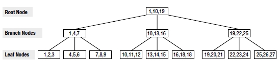
Figure 4-5. B-tree layout of 27 rows
A B-tree consists of a starting node (or page) called a root node with branch nodes (or pages) growing out of it (or linked to it). All keys are stored in the leaves. Contained in each interior node (above the leaf nodes) are pointers to its branch nodes and values representing the smallest value found in the branch node. Keys are kept in sorted order within each node. B-trees use a balanced tree structure for efficient record retrieval—a B-tree is balanced when the leaf nodes are all at the same level from the root node. For example, creating an index on the preceding content will generate the balanced B-tree structure shown in Figure 4-5. At the bottom level, all the leaf nodes are connected to each other through a doubly-linked list, meaning each page points to the page that follows it, and the page that follows it points back to the preceding page. This prevents having to go back up the chain when pages are traversed beyond the definitions of the intermediate pages.
The B-tree algorithm minimizes the number of pages to be accessed to locate a desired key, thereby speeding up the data access process. For example, in Figure 4-5, the search for the key value 5 starts at the top root node. Since the key value is between 1 and 10, the search process follows the left branch to the next node. As the key value 5 falls between the values 4 and 7, the search process follows the middle branch to the next node with the starting key value of 4. The search process retrieves the key value 5 from this leaf page. If the key value 5 doesn’t exist in this page, the search process will stop since it’s the leaf page. Similarly, the key value 25 can also be searched using the same number of reads.
Index Overhead
The performance benefit of indexes does come at a cost. Tables with indexes require more storage and memory space for the index pages in addition to the data pages of the table. Data manipulation queries (INSERT, UPDATE, and DELETE statements, or the CUD part of create, read, update, delete [CRUD]) can take longer, and more processing time is required to maintain the indexes of constantly changing tables. This is because, unlike a SELECT statement, data manipulation queries modify the data content of a table. If an INSERT statement adds a row to the table, then it also has to add a row in the index structure. If the index is a clustered index, the overhead is greater still, because the row has to be added to the data pages themselves in the right order, which may require other data rows to be repositioned below the entry position of the new row. The UPDATE and DELETE data manipulation queries change the index pages in a similar manner.
When designing indexes, you’ll be operating from two different points of view: the existing system, already in production, where you need to measure the overall impact of an index, and the tactical approach where all you worry about is the immediate benefits of an index, usually when initially designing a system. When you have to deal with the existing system, you should ensure that the performance benefits of an index outweigh the extra cost in processing resources. You can do this by using Extended Events (explained in Chapter 3) to do an overall workload optimization (explained in Chapter 16). When you’re focused exclusively on the immediate benefits of an index, SQL Server supplies a series of dynamic management views that provide detailed information about the performance of indexes, sys.dm_db_index_operational_stats or sys.dm_db_index_usage_stats. The view sys.dm_db_index_operational_stats shows the low-level activity, such as locks and I/O, on an index that is in use. The view sys.dm_db_index_usage_stats returns statistical counts of the various index operations that have occurred to an index over time. Both of these will be used more extensively in Chapter 12 when I discuss blocking.
![]() Note Throughout the book, I use the STATISTICS IO and STATISTICS TIME measurements against the queries that we’re running. You can add SET commands to the code, or you can change the connection settings for the query window. I suggest just changing the connection settings.
Note Throughout the book, I use the STATISTICS IO and STATISTICS TIME measurements against the queries that we’re running. You can add SET commands to the code, or you can change the connection settings for the query window. I suggest just changing the connection settings.
To understand the overhead cost of an index on data manipulation queries, consider the following example. First, create a test table with 10,000 rows:
IF (SELECT OBJECT_ID('Test1')
) IS NOT NULL
DROP TABLE dbo.Test1 ;
GO
CREATE TABLE dbo.Test1
(C1 INT,
C2 INT,
C3 VARCHAR(50)
) ;
WITH Nums
AS (SELECT TOP (10000)
ROW_NUMBER() OVER (ORDER BY (SELECT 1
)) AS n
FROM Master.sys.All_Columns ac1
CROSS JOIN Master.sys.ALL_Columns ac2
)
INSERT INTO dbo.Test1
(C1, C2, C3)
SELECT n,
n,
'C3'
FROM Nums;
Run an UPDATE statement, like so:
UPDATE dbo.Test1
SET C1 = 1,
C2 = 1
WHERE C2 = 1 ;
Then the number of logical reads reported by SET STATISTICS I0 is as follows:
Table 'Test1'. Scan count 1, logical reads 29
Add an index on column cl, like so:
CREATE CLUSTERED INDEX iTest
ON dbo.Test1(C1) ;
Then the resultant number of logical reads for the same UPDATE statement increases from 29 to 42:
Table 'Test1'. Scan count 1, logical reads 42
Table 'Worktable'. Scan count 1, logical reads 5
I get to 42 because a worktable was created to help scan through the data, increasing the number of reads beyond what was necessary just because of the incorrect index.
Even though it is true that the amount of overhead required to maintain indexes increases for data manipulation queries, be aware that SQL Server must first find a row before it can update or delete it; therefore, indexes can be helpful for UPDATE and DELETE statements with complex WHERE clauses as well. The increased efficiency in using the index to locate a row usually offsets the extra overhead needed to update the indexes, unless the table has a lot of indexes.
To understand how an index can benefit even data modification queries, let’s build on the example. Create another index on table tl. This time, create the index on column c2 referred to in the WHERE clause of the UPDATE statement:
CREATE INDEX iTest2
ON dbo.Test1(C2) ;
After adding this new index, run the UPDATE command again:
UPDATE dbo.Test1
SET C1 = 1,
C2 = 1
WHERE C2 = 1 ;
The total number of logical reads for this UPDATE statement decreases from 43 to 20 (= 15 + 5):
Table 'Test1'. Scan count 1, logical reads 15
Table 'Worktable'. Scan count 1, logical reads 5
![]() Note A worktable is a temporary table used internally by SQL Server to process the intermediate results of a query. Worktables are created in the tempdb database and are dropped automatically after query execution.
Note A worktable is a temporary table used internally by SQL Server to process the intermediate results of a query. Worktables are created in the tempdb database and are dropped automatically after query execution.
The examples in this section have demonstrated that although having an index adds some overhead cost to action queries, the overall result is a decrease in cost because of the beneficial effect of indexes on searching, even during updates.
The main recommendations for index design are as follows:
- Examine the WHERE clause and JOIN criteria columns.
- Use narrow indexes.
- Examine column uniqueness.
- Examine the column data type.
- Consider column order.
- Consider the type of index (clustered vs. nonclustered).
Let’s consider each of these recommendations in turn.
Examine the WHERE Clause and JOIN Criteria Columns
When a query is submitted to SQL Server, the query optimizer tries to find the best data access mechanism for every table referred to in the query. Here is how it does this:
1. The optimizer identifies the columns included in the E Clause and JOIN Criteria CWHERE clause and the JOIN criteria.
2. The optimizer then examines indexes on those columns.
3. The optimizer assesses the usefulness of each index by determining the selectivity of the clause (that is, how many rows will be returned) from statistics maintained on the index.
4. Finally, the optimizer estimates the least costly method of retrieving the qualifying rows, based on the information gathered in the previous steps.
![]() Note Chapter 7 covers statistics in more depth.
Note Chapter 7 covers statistics in more depth.
To understand the significance of a WHERE clause column in a query, let’s consider an example. Let’s return to the original code listing that helped you understand what an index is; the query consisted of a SELECT statement without any WHERE clause, as follows:
SELECT p.ProductID,
p.Name,
p.StandardCost,
p.Weight
FROM Production.Product p ;
The query optimizer performs a clustered index scan, the equivalent of a table scan against a heap on a table that has a clustered index, to read the rows as shown in Figure 4-6 (switch on the Include Actual Execution Plan option by using Ctrl-M inside a query window, as well as the Set Statistics I0 option by right-clicking and selecting Query Options and then selecting the appropriate check box in the Advanced tab).
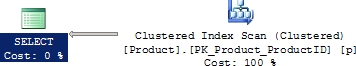
Figure 4-6. Execution plan with no WHERE clause
The number of logical reads reported by SET STATISTICS I0 for the SELECT statement is as follows:
Table 'Product'. Scan count 1, logical reads 15
To understand the effect of a WHERE clause column on the query optimizer’s decision, let’s add a WHERE clause to retrieve a single row:
SELECT p.ProductID,
p.Name,
p.StandardCost,
p.Weight
FROM Production.Product AS p
WHERE p.ProductID = 738 ;
With the WHERE clause in place, the query optimizer examines the WHERE clause column ProductID, identifies the availability of index PK Product ProductId on column Productld, assesses a high selectivity (that is, only one row will be returned) for the WHERE clause from the statistics on index PK Product Productld, and decides to use that index on column Productld, as shown in Figure 4-7.
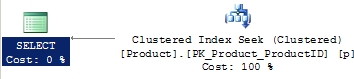
Figure 4-7. Execution plan with a WHERE clause
The resultant number of logical reads is as follows:
Table 'Product'. Scan count 0, logical reads 2
The behavior of the query optimizer shows that the WHERE clause column helps the optimizer choose an optimal indexing operation for a query. This is also applicable for a column used in the JOIN criteria between two tables. The optimizer looks for the indexes on the WHERE clause column or the JOIN criterion column and, if available, considers using the index to retrieve the rows from the table. The query optimizer considers index(es) on the WHERE clause column(s) and the JOIN criteria column(s) while executing a query. Therefore, having indexes on the frequently used columns in the WHERE clause and the JOIN criteria of a SQL query helps the optimizer avoid scanning a base table.
When the amount of data inside a table is so small that it fits onto a single page (8KB), a table scan may work better than an index seek. If you have a good index in place but you’re still getting a scan, consider this issue.
For best performance, you should use as narrow a data type as possible when creating indexes. Narrow in this context means as small a data type as you can. You should also avoid very wide data type columns in an index. Columns with string data types (CHAR, VARCHAR, NCHAR, and NVARCHAR) sometimes can be quite wide as can binary and globally unique identifiers (GUID). Unless they are absolutely necessary, minimize the use of wide data type columns with large sizes in an index. You can create indexes on a combination of columns in a table. For the best performance, use as few columns in an index as you can.
A narrow index can accommodate more rows in an 8KB index page than a wide index. This has the following effects:
- Reduces I/O (by having to read fewer 8KB pages)
- Makes database caching more effective, because SQL Server can cache fewer index pages, consequently reducing the logical reads required for the index pages in the memory
- Reduces the storage space for the database
To understand how a narrow index can reduce the number of logical reads, create a test table with 20 rows and an index:
IF (SELECT OBJECT_ID('Test1')
) IS NOT NULL
DROP TABLE dbo.Test1 ;
GO
CREATE TABLE dbo.Test1 (C1 INT, C2 INT) ;
WITH Nums
AS (SELECT 1 AS n
UNION ALL
SELECT n + 1
FROM Nums
WHERE n < 20
)
INSERT INTO dbo.Test1
(C1, C2)
SELECT n,
2
FROM Nums ;
CREATE INDEX iTest ON dbo.Test1(C1) ;
Since the indexed column is narrow (the INT data type is 4 bytes), all the index rows can be accommodated in one 8KB index page. As shown in Figure 4-8, you can confirm this in the dynamic management views associated with indexes:
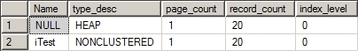
Figure 4-8. Number of pages for a narrow, nonclustered index
SELECT i.Name,
i.type_desc,
ddips.page_count,
ddips.record_count,
ddips.index_level
FROM sys.indexes i
JOIN sys.dm_db_index_physical_stats(DB_ID(N'AdventureWorks2008R2'),
OBJECT_ID(N'dbo.Test1'),
NULL, NULL,
'DETAILED') AS ddips
ON i.index_id = ddips.index_id
WHERE i.object_id = OBJECT_ID(N'dbo.Test1') ;
The sys.indexes system table is stored in each database and contains the basic information on every index in the database. The dynamic management function, sys.dm_db_index_ physical_stats, contains the more detailed information about the statistics on the index (you’ll learn more about this DMF in Chapter 7). To understand the disadvantage of a wide index key, modify the data type of the indexed column cl from INT to CHAR(500) (narrow_ alter.sql in the download):
DROP INDEX dbo.Test1.iTest ;
ALTER TABLE dbo.Test1 ALTER COLUMN C1 CHAR(500) ;
CREATE INDEX iTest ON dbo.Test1(C1) ;
The width of a column with the INT data type is 4 bytes, and the width of a column with the CHAR(500) data type is 500 bytes. Because of the large width of the indexed column, two index pages are required to contain all 20 index rows. You can confirm this in the sys.dm_db_index_physical_stats dynamic management function by running the query against it again (see Figure 4-9).
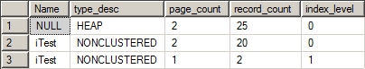
Figure 4-9. Number of pages for a wide, nonclustered index
A large index key size increases the number of index pages, thereby increasing the amount of memory and disk activities required for the index. It is always recommended that the index key size is as narrow as possible.
Drop the test table before continuing:
DROP TABLE dbo.Test1;
Examine Column Uniqueness
Creating an index on columns with a very low range of possible unique values (such as gender) will not benefit performance, because the query optimizer will not be able to use the index to effectively narrow down the rows to be returned. Consider a Gender column with only two unique values: M and F. When you execute a query with the Gender column in the WHERE clause, you end up with a large number of rows from the table (assuming the distribution of M and F is relatively even), resulting in a costly table or clustered index scan. It is always preferable to have columns in the WHERE clause with lots of unique rows (or high selectivity) to limit the number of rows accessed. You should create an index on those column(s) to help the optimizer access a small result set.
Furthermore, while creating an index on multiple columns, which is also referred to as a composite index, column order matters. In some cases, using the most selective column first will help filter the index rows more efficiently.
![]() Note The importance of column order in a composite index is explained later in the chapter in the “Consider Column Order” section.
Note The importance of column order in a composite index is explained later in the chapter in the “Consider Column Order” section.
From this, you can see that it is important to know the selectivity of a column before creating an index on it. You can find this by executing a query like this one; just substitute the table and column name:
SELECT COUNT(DISTINCT e.Gender) AS DistinctColValues,
COUNT(e.Gender) AS NumberOfRows,
(CAST(COUNT(DISTINCT e.Gender) AS DECIMAL)
/ CAST(COUNT(e.Gender) AS DECIMAL)) AS Selectivity
FROM HumanResources.Employee AS e ;
The column with the highest number of unique values (or selectivity) can be the best candidate for indexing when referred to in a WHERE clause or a join criterion. You may also have the exceptional data where you have hundreds of rows of common data with only a few that are unique. The few will also benefit from an index. You can make this even more beneficial by using filtered indexes (discussed in more detail later).
To understand how the selectivity of an index key column affects the use of the index, take a look at the Gender column in the HumanResources.Employee table. If you run the previous query, you’ll see that it contains only two distinct values in more than 290 rows, which is a selectivity of .006. A query to look only for a Gender of
F would look like this:
SELECT e.*
FROM HumanResources.Employee AS e
WHERE e.Gender = 'F'
AND e.SickLeaveHours = 59
AND e.MaritalStatus = 'M' ;
This results in the execution plan in Figure 4-10 and the following I/O and elapsed time:
![]()
Figure 4-10. Execution plan with no index
Table 'Employee'. Scan count 1, logical reads 9
CPU time = 15 ms, elapsed time = 135 ms.
The data is returned by scanning the clustered index (where the data is stored) to find the appropriate values where Gender = 'F'. (The other operators will be covered in Chapter 9.) If you were to place an index on the column, like so, and run the query again, the execution plan remains the same.
CREATE INDEX IX_Employee_Test ON HumanResources.Employee (Gender) ;
The data is just not selective enough for the index to be used, let alone be useful. If instead you use a composite index that looks like this:
CREATE INDEX IX_Employee_Test ON
HumanResources.Employee (SickLeaveHours, Gender, MaritalStatus)
WITH (DROP_EXISTING = ON) ;
and then rerun the query to see the execution plan in Figure 4-11 and the performance results, you get this:
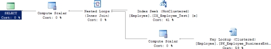
Figure 4-11. Execution plan with a composite index
Table 'Employee'. Scan count 1, logical reads 6
CPU time = 0 ms, elapsed time = 32 ms.
Now you’re doing better than you were with the clustered index scan. A nice clean Index Seek operation takes about half the time to gather the data. The rest is spent in the Key Lookup operation. A Key Lookup operation is commonly referred to as a bookmark lookup.
![]() Note You will learn more about bookmark lookups in Chapter 6.
Note You will learn more about bookmark lookups in Chapter 6.
Although none of the columns in question would probably be selective enough on their own to make a decent index, together they provide enough selectivity for the optimizer to take advantage of the index offered.
It is possible to attempt to force the query to use the first test index you created. If you drop the compound index, create the original again, and then modify the query as follows by using a query hint to force the use of the original index:
SELECT e.*
FROM HumanResources.Employee AS e WITH (INDEX (IX_Employee_Test))
WHERE e.SickLeaveHours = 59
AND e.Gender = 'F'
AND e.MaritalStatus = 'M' ;
then the results and execution plan shown in Figure 4-12, while similar, are not the same:

Figure 4-12. Execution plan when the index is chosen with a query hint
Table 'Employee'. Scan count 1, logical reads 170
CPU time = 0 ms, elapsed time = 55 ms.
You see the same index seek, but the number of reads has more than doubled, and the estimated costs within the execution plan have changed. Although forcing the optimizer to choose an index is possible, it clearly isn’t always an optimal approach.
Another way to force a different behavior on SQL Server 2012 is the FORCESEEK query hint. FORCESEEK makes it so the optimizer will choose only Index Seek operations. If the query were rewritten like this:
SELECT e.*
FROM HumanResources.Employee AS e WITH (FORCESEEK)
WHERE e.SickLeaveHours = 59
AND e.Gender = 'F'
AND e.MaritalStatus = 'M' ;
which changes the I/O, execution time, and execution plan results yet again (Figure 4-13), you end up with these results:
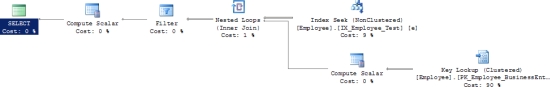
Figure 4-13. Forcing a Seek operation using FORCESEEK query hint
Table 'Employee'. Scan count 1, logical reads 170
CPU time = 0 ms, elapsed time = 66 ms.
Limiting the options of the optimizer and forcing behaviors can in some situations help, but frequently, as shown with the results here, an increase in execution time and the number of reads is not helpful.
![]() Note To make the best use of your indexes, it is highly recommended that you create the index on a column (or set of columns) with very high selectivity.
Note To make the best use of your indexes, it is highly recommended that you create the index on a column (or set of columns) with very high selectivity.
Before moving on, be sure to drop the test index from the table:
DROP INDEX HumanResources.Employee.IX_Employee_Test;
Examine the Column Data Type
The data type of an index matters. For example, an index search on integer keys is very fast because of the small size and easy arithmetic manipulation of the INTEGER (or INT) data type. You can also use other variations of integer data types (BIGINT, SMALLINT, and TINYINT) for index columns, whereas string data types (CHAR, VARCHAR, NCHAR, and NVARCHAR) require a string match operation, which is usually costlier than an integer match operation.
Suppose you want to create an index on one column and you have two candidate columns—one with an INTEGER data type and the other with a CHAR(4) data type. Even though the size of both data types is 4 bytes in SQL Server 2012, you should still prefer the INTEGER data type index. Look at arithmetic operations as an example. The value 1 in the CHAR(4) data type is actually stored as 1 followed by three spaces, a combination of the following four bytes: 0x35, 0x20, 0x20, and 0x20. The CPU doesn’t understand how to perform arithmetic operations on this data, and therefore it converts to an integer data type before the arithmetic operations, whereas the value 1 in an integer data type is saved as 0x00000001. The CPU can easily perform arithmetic operations on this data.
Of course, most of the time, you won’t have the simple choice between identically sized data types, allowing you to choose the more optimal type. Keep this information in mind when designing and building your indexes.
Consider Column Order
An index key is sorted on the first column of the index and then subsorted on the next column within each value of the previous column. The first column in a compound index is frequently referred to as the leading edge of the index. For example, consider Table 4-2.
If a composite index is created on the columns (c1, c2), then the index will be ordered as shown in Table 4-3.
As shown in Table 4-3, the data is sorted on the first column (cl) in the composite index. Within each value of the first column, the data is further sorted on the second column (c2).
Therefore, the column order in a composite index is an important factor in the effectiveness of the index. You can see this by considering the following:
- Column uniqueness
- Column width
- Column data type
For example, suppose most of your queries on table t1 are similar to the following:
SELECT * FROM t1 WHERE c2=12 ;
SELECT * FROM t1 WHERE c2=12 AND c1=ll ;
Table 4-2. Sample Table
| c1 | c2 |
| 1 | 1 |
| 2 | 1 |
| 3 | 1 |
| 1 | 2 |
| 2 | 2 |
| 3 | 2 |
Table 4-3. Composite Index on Columns (cl, c2)
| c1 | c2 |
| 1 | 1 |
| 1 | 2 |
| 2 | 1 |
| 2 | 2 |
| 3 | 1 |
| 3 | 2 |
An index on (c2, c1) will benefit both the queries. But an index on (cl, c2) will not be helpful to both queries, because it will sort the data initially on column cl, whereas the first SELECT statement needs the data to be sorted on column c2.
To understand the importance of column ordering in an index, consider the following example. In the Person.Address table, there is a column for City and another for PostalCode. Create an index on the table like this:
CREATE INDEX IX_Test ON Person.Address (City, PostalCode) ;
A simple SELECT statement run against the table that will use this new index will look something like this:
SELECT a.*
FROM Person.Address AS a
WHERE a.City = 'Warrington' ;
The I/O and execution time for the query is as follows:
Table 'Address'. Scan count 1, logical reads 188
CPU time = 0 ms, elapsed time = 186 ms.
And the execution plan in Figure 4-14 shows the use of the index.
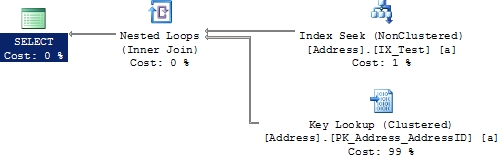
Figure 4-14. Execution plan for query against leading edge of index
So, this query is taking advantage of the leading edge of the index to perform a Seek operation to retrieve the data. If, instead of querying using the leading edge, you use another column in the index like the following query:
SELECT *
FROM Person.Address AS a
WHERE a.PostalCode = 'WA3 7BH' ;
then the results are as follows:
Table 'Address'. Scan count 1, logical reads 180
CPU time = 16 ms, elapsed time = 249 ms.
And the execution plan is clearly different, as you can see in Figure 4-15.
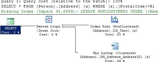
Figure 4-15. Execution plan for query against inner columns
The reads for the second query are slightly lower than the first, but when you take into account that the first query returned 86 rows worth of data and the second query returned only 31, you begin to see the difference between the Index Seek operation in Figure 4-14 and the Index Scan operation in Figure 4-15. Also note that because it had to perform a scan, the optimizer marked the column as possibly missing an index.
Missing index information is useful as a pointer to the potential for a new or better index on a table, but don’t assume it’s always correct. You can right-click the place where the missing index information is and select “Missing Index Details…” from the context menu. That will open a new query window with the details of the index laid out, ready for creation. If you do decide to test that index, make sure you rename it from the default name.
Finally, to see the order of the index really shine, change the query to this:
SELECT a.AddressID,
a.City,
a.PostalCode
FROM Person.Address AS a
WHERE a.City = 'Warrington'
AND a.PostalCode = 'WA3 7BH' ;
Executing this query will return the same 31 rows as the previous query, resulting in the following:
Table 'Address'. Scan count 1, logical reads 2
CPU time = 0 ms, elapsed time = 0 ms.
The execution plan is visible in Figure 4-16.
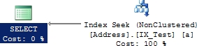
Figure 4-16. Execution plan using both columns
The radical changes in I/O and execution plan represent the real use of a compound index, the covering index. This is covered in detail in the section “Covering Indexes” later in the chapter.
When finished, drop the index:
DROP INDEX Person.Address.IX_Test
Consider the Type of Index
In SQL Server, from all the different types of indexes available to you, most of the time you’ll be working with the two main index types: clustered and nonclustered. Both types have a B-tree structure. The main difference between the two types is that the leaf pages in a clustered index are the data pages of the table and are therefore in the same order as the data to which they point. This means that the clustered index is the table. As you proceed, you will see that the difference at the leaf level between the two index types becomes very important when determining the type of index to use.
Clustered Indexes
The leaf pages of a clustered index and the data pages of the table the index is on are one and the same. Because of this, table rows are physically sorted on the clustered index column, and since there can be only one physical order of the table data, a table can have only one clustered index.
![]() Tip When you create a primary key constraint, SQL Server automatically creates it as a unique clustered index on the primary key if one does not already exist and if it is not explicitly specified that the index should be a unique nonclustered index. This is not a requirement; it’s just default behavior. You can change the primary key prior to creating the table.
Tip When you create a primary key constraint, SQL Server automatically creates it as a unique clustered index on the primary key if one does not already exist and if it is not explicitly specified that the index should be a unique nonclustered index. This is not a requirement; it’s just default behavior. You can change the primary key prior to creating the table.
As mentioned earlier in the chapter, a table with no clustered index is called a heap table. The data rows of a heap table are not stored in any particular order or linked to the adjacent pages in the table. This unorganized structure of the heap table usually increases the overhead of accessing a large heap table when compared to accessing a large nonheap table (a table with a clustered index).
Relationship with Nonclustered Indexes
There is an interesting relationship between a clustered index and the nonclustered indexes in SQL Server. An index row of a nonclustered index contains a pointer to the corresponding data row of the table. This pointer is called a row locator. The value of the row locator depends on whether the data pages are stored in a heap or are clustered. For a nonclustered index, the row locator is a pointer to the RID for the data row in a heap. For a table with a clustered index, the row locator is the clustered index key value.
For example, say you have a heap table with no clustered index, as shown in Table 4-4.
Table 4-4. Data Page for a Sample Table
| RowID (Not a Real Column) | c1 | c2 | c3 |
| 1 | A1 | A2 | A3 |
| 2 | B1 | B2 | B3 |
A nonclustered index on column c1 in a heap will cause the row locator for the index rows to contain a pointer to the corresponding data row in the database table, as shown in Table 4-5.
Table 4-5. Nonclustered Index Page with No Clustered Index
| c1 | Row Locator |
| A1 | Pointer to RID = 1 |
| B1 | Pointer to RID = 2 |
On creating a clustered index on column c2, the row locator values of the nonclustered index rows are changed. The new value of the row locator will contain the clustered index key value, as shown in Table 4-6.
Table 4-6. Nonclustered Index Page with a Clustered Index on c2
| c1 | Row Locator |
| A1 | A2 |
| B1 | B2 |
To verify this dependency between a clustered and a nonclustered index, let’s consider an example. In the AdventureWorks2008R2 database, the table dbo.DatabaseLog contains no clustered index, just a nonclustered primary key. If a query is run against it like the following, then the execution will look like Figure 4-17.
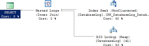
Figure 4-17. Execution plan against a heap
SELECT dl.DatabaseLogID,
dl.PostTime
FROM dbo.DatabaseLog AS dl
WHERE dl.DatabaseLogID = 115 ;
As you can see, the index was used in a Seek operation. But because the data is stored separately from the nonclustered index, an additional operation, the RID Lookup operation, is required in order to retrieve the data, which is then joined back to the information from the Index Seek operation through a Nested Loop operation. This is a classic example of what is known as a bookmark lookup, which is explained in more detail in the “Defining the Bookmark Lookup” section. A similar query run against a table with a clustered index in place will look like this:
SELECT d.DepartmentID,
d.ModifiedDate
FROM HumanResources.Department AS d
WHERE d.DepartmentID = 10 ;
Figure 4-18 shows this execution plan returned.
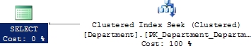
Figure 4-18. Execution plan with a clustered index
Although the primary key is used in the same way as the previous query, this time it’s against a clustered index. As you now know, this means the data is stored with the index, so the additional column doesn’t require a lookup operation to get the data. Everything is returned by the simple clustered Index Seek operation.
To navigate from a nonclustered index row to a data row, this relationship between the two index types requires an additional indirection for navigating the B-tree structure of the clustered index. Without the clustered index, the row locator of the nonclustered index would be able to navigate directly from the nonclustered index row to the data row in the base table. The presence of the clustered index causes the navigation from the nonclustered index row to the data row to go through the B-tree structure of the clustered index, since the new row locator value points to the clustered index key.
On the other hand, consider inserting an intermediate row in the clustered index key order or expanding the content of an intermediate row. For example, imagine a clustered index table containing four rows per page, with clustered index column values of 1, 2, 4, and 5. Adding a new row in the table with the clustered index value 3 will require space in the page between values 2 and 4. If enough space is not available in that position, a page split will occur on the data page (or clustered index leaf page). Even though the data page split will cause relocation of the data rows, the nonclustered index row locator values need not be updated. These row locators continue to point to the same logical key values of the clustered index key, even though the data rows have physically moved to a different location. In the case of a data page split, the row locators of the nonclustered indexes need not be updated. This is an important point, since tables often have a large number of nonclustered indexes.
Things don’t work the same way for heap tables. While page splits are not a common practice, anything that causes the location of the heap pages to change automatically requires that the nonclustered indexes get immediately updated.
![]() Note Page splits and their effect on performance are explained in more detail in Chapter 8.
Note Page splits and their effect on performance are explained in more detail in Chapter 8.
Clustered Index Recommendations
The relationship between a clustered index and a nonclustered index imposes some considerations on the clustered index, which are explained in the sections that follow.
Create the Clustered Index First
Since all nonclustered indexes hold clustered index keys within their index rows, the order of nonclustered and clustered index creation is very important. For example, if the nonclustered indexes are built before the clustered index is created, then the nonclustered index row locator will contain a pointer to the corresponding RID of the table. Creating the clustered index later will modify all the nonclustered indexes to contain clustered index keys as the new row locator value. This effectively rebuilds all the nonclustered indexes.
For the best performance, I recommend that you create the clustered index before you create any nonclustered index. This allows the nonclustered indexes to have their row locator set to the clustered index keys at the time of creation. This does not have any effect on the final performance, but rebuilding the indexes may be quite a large job.
I would also suggest that you design the tables in your database around the clustered index. It should be the first index created because you should be storing your data as a clustered index by default.
Keep Indexes Narrow
Since all nonclustered indexes hold the clustered keys as their row locator, for the best performance keep the overall byte size of the clustered index as small as possible. If you create a wide clustered index, say CHAR(500), this will add 500 bytes to every nonclustered index. Thus, keep the number of columns in the clustered index to a minimum, and carefully consider the byte size of each column to be included in the clustered index. A column of the integer data type often makes a good candidate for a clustered index, whereas a string data type column will be a less-than-optimal choice.
To understand the effect of a wide clustered index on a nonclustered index, consider this example. Create a small test table with a clustered index and a nonclustered index:
IF (SELECT OBJECT_ID(‘Test1')
) IS NOT NULL
DROP TABLE dbo.Test1 ;
GO
CREATE TABLE dbo.Test1 (C1 INT, C2 INT) ;
WITH Nums
AS (SELECT TOP (20)
ROW_NUMBER() OVER (ORDER BY (SELECT 1)) AS n
FROM Master.sys.All_Columns ac1
CROSS JOIN Master.sys.ALL_Columns ac2
)
INSERT INTO dbo.Test1
(C1, C2)
SELECT n,
n + 1
FROM Nums ;
CREATE CLUSTERED INDEX iClustered
ON dbo.Test1 (C2) ;
CREATE NONCLUSTERED INDEX iNonClustered
ON dbo.Test1 (C1) ;
Since the table has a clustered index, the row locator of the nonclustered index contains the clustered index key value—therefore:
Width of the nonclustered index row = width of the nonclustered index column + width of the clustered index column = size of INT data type + size of INT data type
= 4 bytes + 4 bytes = 8 bytes
With this small size of a nonclustered index row, all the rows can be stored in one index page. You can confirm this by querying against the index statistics as shown in Figure 4-19.
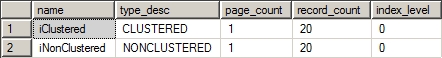
Figure 4-19. Number of index pages for a narrow index
SELECT i.name,
i.type_desc,
s.page_count,
s.record_count,
s.index_level
FROM sys.indexes i
JOIN sys.dm_db_index_physical_stats(DB_ID(N'AdventureWorks2008R2'),
OBJECT_ID(N'dbo.Test1'), NULL,
NULL,
DETAILED') AS s
ON i.index_id = s.index_id
WHERE i.object_id = OBJECT_ID(N'dbo.Test1') ;
To understand the effect of a wide clustered index on a nonclustered index, modify the data type of the clustered indexed column c2 from INT to CHAR(500):
DROP INDEX dbo.Test1.iClustered ;
ALTER TABLE dbo.Test1 ALTER COLUMN C2 CHAR(500) ;
CREATE CLUSTERED INDEX iClustered ON dbo.Test1(C2) ;
Running the query against sys.dm_db_index_physical_stats again returns the result in Figure 4-20.
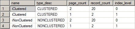
Figure 4-20. Number of index pages for a wide index
You can see that a wide clustered index increases the width of the nonclustered index row size. Because of the large width of the nonclustered index row, one 8KB index page can’t accommodate all the index rows. Instead, two index pages will be required to store all 20 index rows. In the case of a large table, an expansion in the size of the nonclustered indexes because of a large clustered index key size can significantly increase the number of pages of the nonclustered indexes.
Therefore, a large clustered index key size not only affects its own width but also widens all nonclustered indexes on the table. This increases the number of index pages for all the indexes on the table, increasing the logical reads and disk I/Os required for the indexes.
Rebuild the Clustered Index in a Single Step
Because of the dependency of nonclustered indexes on the clustered index, rebuilding the clustered index as separate DROP INDEX and CREATE INDEX statements causes all the nonclustered indexes to be rebuilt twice. To avoid this, use the DROP_EXISTING clause of the CREATE INDEX statement to rebuild the clustered index in a single atomic step. Similarly, you can also use the DROP_EXISTING clause with a nonclustered index.
It’s worth noting that in SQL Server 2005 and better, when you perform a straight rebuild of a clustered index, you won’t see the clustered indexes rebuilt as well.
When to Use a Clustered Index
In certain situations, using a clustered index is very helpful. I discuss these in the sections that follow.
Accessing the Data Directly
With all the data stored on the leaf pages of a clustered index, any time you access the cluster, the data is immediately available. One use for a clustered index is to support the most commonly used access path to the data. Any access of the clustered index does not require any additional reads to retrieve the data, which means seeks or scans against the clustered index do not require any additional reads to retrieve that data. This is the likely reason that Microsoft has made the primary key a clustered index by default. Since the primary key is frequently the most likely means of accessing data in a table, it serves well as a clustered index.
Just remember that the primary key being the clustered index is a default behavior, but not necessarily the most common access path to the data. This could be through foreign key constraints, alternate keys in the table, or other columns. Plan and design the cluster with storage and access in mind, and you should be fine.
The clustered index works well as the primary path to the data only if you’re accessing a considerable portion of the data within a table. If, on the other hand, you’re accessing small subsets of the data, you might be better off with a nonclustered covering index. Also, you have to take into account the number and types of columns that define the access path to the data. Since the key of a clustered index becomes the pointer for nonclustered indexes, excessively wide clustered keys can seriously impact performance and storage for nonclustered indexes.
Clustered indexes are particularly efficient when the data retrieval needs to be sorted. If you create a clustered index on the column or columns that you may need to sort by, then the rows will be physically stored in that order, eliminating the overhead of sorting the data after it is retrieved.
Let’s see this in action. Create a test table as follows (createsort.sql in the download):
IF (SELECT OBJECT_ID('od')
) IS NOT NULL
DROP TABLE dbo.od ;
GO
SELECT pod.*
INTO dbo.od
FROM Purchasing.PurchaseOrderDetail AS pod ;
The new table od is created with data only. It doesn’t have any indexes. You can verify the indexes on the table by executing the following, which returns nothing:
EXEC sp_helpindex 'dbo.od' ;
To understand the use of a clustered index, fetch a large range of rows ordered on a certain column:
SELECT od.*
FROM dbo.od
WHERE od.ProductID BETWEEN 500 AND 510
ORDER BY od.ProductID ;
You can obtain the cost of executing this query (without any indexes) from the STATISTICS IO output:
Table 'od'. Scan count 1, logical reads 78
To improve the performance of this query, you should create an index on the WHERE clause column. This query requires both a range of rows and a sorted output. The result set requirement of this query meets the recommendations for a clustered index. Therefore, create a clustered index as follows, and reexamine the cost of the query:
CREATE CLUSTERED INDEX i1 ON od(ProductID) ;
When you run the query again, the resultant cost of the query (with a clustered index) is as follows:
Table 'od'. Scan count 1, logical reads 8
Creating the clustered index reduced the number of logical reads and therefore should contribute to the query performance improvement.
On the other hand, if you create a nonclustered index (instead of a clustered index) on the candidate column, then the query performance may be affected adversely. Let’s verify the effect of a nonclustered index in this case:
DROP INDEX od.i1 ;
CREATE NONCLUSTERED INDEX i1 on dbo.od(ProductID) ;
The resultant cost of the query (with a nonclustered index) is as follows:
Table 'od'. Scan count 1, logical reads 87
The nonclustered index significantly increases the number of logical reads. There was also an increase in query performance, probably related to the increase in reads. Drop the test table when you’re done:
DROP TABLE dbo.od ;
Poor Design Practices for a Clustered Index
In certain situations, you are better off not using a clustered index. I discuss these in the sections that follow.
If the clustered index columns are frequently updated, this will cause the row locator of all the nonclustered indexes to be updated accordingly, significantly increasing the cost of the relevant action queries. This also affects database concurrency by blocking all other queries referring to the same part of the table and the nonclustered indexes during that period. Therefore, avoid creating a clustered index on columns that are highly updatable.
![]() Note Chapter 12 covers blocking in more depth.
Note Chapter 12 covers blocking in more depth.
To understand how the cost of an UPDATE statement that modifies only a clustered key column is increased by the presence of nonclustered indexes on the table, consider the following example. The Sales.SpecialOfferProduct table has a composite clustered index on the primary key, which is also the foreign key from two different tables; this is a classic many-to-many join. In this example, I update one of the two columns using the following statement (note the use of the transaction to keep the test data intact):
BEGIN TRAN
SET STATISTICS IO ON ;
UPDATE Sales.SpecialOfferProduct
SET ProductID = 345
WHERE SpecialOfferID = 1
AND ProductID = 720 ;
SET STATISTICS IO OFF ;
ROLLBACK TRAN
The STATISTICS IO output shows the reads necessary:
Table 'Product'. Scan count 0, logical reads 2
Table 'SalesOrderDetail'. Scan count 1, logical reads 1240
Table 'SpecialOfferProduct'. Scan count 0, logical reads 15
If you added a nonclustered index to the table, you would see the reads increase:
CREATE NONCLUSTERED INDEX ixTest
ON Sales.SpecialOfferProduct (ModifiedDate) ;
When you run the same query again, the output of STATISTICS IO changes for the SpecialOfferProduct table:
Table 'Product'. Scan count 0, logical reads 2, physical re
Table 'SalesOrderDetail'. Scan count 1, logical reads 1240,
Table 'SpecialOfferProduct'. Scan count 0, logical reads 19
As you can see, the number of reads caused by the update of the clustered index is increased with the addition of the nonclustered index. Be sure to drop the index:
DROP INDEX Sales.SpecialOfferProduct.ixTest ;
Since all nonclustered indexes hold the clustered keys as their row locator, for performance reasons you should avoid creating a clustered index on a very wide column (or columns) or on too many columns. As explained in the preceding section, a clustered index must be as narrow as possible.
Nonclustered Indexes
A nonclustered index does not affect the order of the data in the table pages, because the leaf pages of a nonclustered index and the data pages of the table are separate. A pointer (the row locator) is required to navigate from an index row to the data row. As you learned in the earlier “Clustered Indexes” section, the structure of the row locator depends on whether the data pages are stored in a heap or a clustered index. For a heap, the row locator is a pointer to the RID for the data row; for a table with a clustered index, the row locator is the clustered index key.
Nonclustered Index Maintenance
The row locator value of the nonclustered indexes continues to have the same clustered index value, even when the clustered index rows are physically relocated.
In a table that is a heap, where there is no clustered index, to optimize this maintenance cost, SQL Server adds a pointer to the old data page to point to the new data page after a page split, instead of updating the row locator of all the relevant nonclustered indexes. Although this reduces the maintenance cost of the nonclustered indexes, it increases the navigation cost from the nonclustered index row to the data row within the heap, since an extra link is added between the old data page and the new data page. Therefore, having a clustered index as the row locator decreases this overhead associated with the nonclustered index.
Defining the Bookmark Lookup
When a query requests columns that are not part of the nonclustered index chosen by the optimizer, a lookup is required. This may be a key lookup when going against a clustered index or an RID lookup when performed against a heap. The common term for these lookups comes from the old definition name, bookmark lookup. The lookup fetches the corresponding data row from the table by following the row locator value from the index row, requiring a logical read on the data page besides the logical read on the index page. However, if all the columns required by the query are available in the index itself, then access to the data page is not required. This is known as a covering index.
These lookups are the reason that large result sets are better served with a clustered index. A clustered index doesn’t require a bookmark lookup, since the leaf pages and data pages for a clustered index are the same.
![]() Note Chapter 6 covers lookup operations in more detail.
Note Chapter 6 covers lookup operations in more detail.
Nonclustered Index Recommendations
Since a table can have only one clustered index, you can use the flexibility of multiple nonclustered indexes to help improve performance. I explain the factors that decide the use of a nonclustered index in the following sections.
When to Use a Nonclustered Index
A nonclustered index is most useful when all you want to do is retrieve a small number of rows and columns from a large table. As the number of columns to be retrieved increases, the ability to have a covering index decreases. Then, if you’re also retrieving a large number of rows, the overhead cost of the bookmark lookup rises proportionately. To retrieve a small number of rows from a table, the indexed column should have a very high selectivity.
Furthermore, there will be indexing requirements that won’t be suitable for a clustered index, as explained in the “Clustered Indexes” section:
- Frequently updatable columns
- Wide keys
In these cases, you can use a nonclustered index, since, unlike a clustered index, it doesn’t affect other indexes in the table. A nonclustered index on a frequently updatable column isn’t as costly as having a clustered index on that column. The UPDATE operation on a nonclustered index is limited to the base table and the nonclustered index. It doesn’t affect any other nonclustered indexes on the table. Similarly, a nonclustered index on a wide column (or set of columns) doesn’t increase the size of any other index, unlike that with a clustered index. However, remain cautious, even while creating a nonclustered index on a highly updatable column or a wide column (or set of columns), since this can increase the cost of action queries, as explained earlier in the chapter.
![]() Tip A nonclustered index can also help resolve blocking and deadlock issues. I cover this in more depth in Chapters 12 and 13.
Tip A nonclustered index can also help resolve blocking and deadlock issues. I cover this in more depth in Chapters 12 and 13.
When Not to Use a Nonclustered Index
Nonclustered indexes are not suitable for queries that retrieve a large number of rows. Such queries are better served with a clustered index, which doesn’t require a separate bookmark lookup to retrieve a data row. Since a bookmark lookup requires additional logical reads to get to the data page besides the logical read on the nonclustered index page, the cost of a query using a nonclustered index increases significantly for a large number of rows, such as when in a loop join that requires one lookup after another. The SQL Server query optimizer takes this cost into effect and accordingly can discard the nonclustered index when retrieving a large result set.
If your requirement is to retrieve a large result set from a table, then having a nonclustered index on the filter criterion (or the join criterion) column will probably not be useful unless you use a special type of nonclustered index called a covering index. I describe this index type in detail later in the chapter.
Clustered vs. Nonclustered Indexes
The main considerations in choosing between a clustered and a nonclustered index are as follows:
- Number of rows to be retrieved
- Data-ordering requirement
- Index key width
- Column update frequency
- Lookup cost
- Any disk hot spots
Benefits of a Clustered Index over a Nonclustered Index
When deciding upon a type of index on a table with no indexes, the clustered index is usually the preferred choice. Because the index page and the data pages are the same, the clustered index doesn’t have to jump from the index row to the base row as required in the case of a non-covering nonclustered index.
To understand how a clustered index can outperform a nonclustered index in these circumstances, even in retrieving a small number of rows, create a test table with a high selectivity for one column:
IF (SELECT OBJECT_ID('dbo.Test1')
) IS NOT NULL
DROP TABLE dbo.Test1 ;
GO
CREATE TABLE dbo.Test1 (C1 INT, C2 INT) ;
WITH Nums
AS (SELECT TOP (10000)
ROW_NUMBER() OVER (ORDER BY (SELECT 1)) AS n
FROM Master.sys.all_columns AS ac1
CROSS JOIN Master.sys.all_columns AS ac2
)
INSERT INTO dbo.Test1
(C1, C2)
SELECT n,
2
FROM Nums ;
The following SELECT statement fetches only 1 out of 10,000 rows from the table:
SELECT t.C1,
t. C2
FROM dbo.Test1 AS t
WHERE C1 = 1000 ;
This will be with the graphical execution plan shown in Figure 4-21 and the output of SET STATISTICS IO as follows:
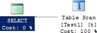
Figure 4-21. Execution plan with no index
Table 'Test1'. Scan count 1, logical reads 22
Considering the small size of the result set retrieved by the preceding SELECT statement, a nonclustered column on c1 can be a good choice:
CREATE NONCLUSTERED INDEX incl ON dbo.Test1(C1) ;
You can run the same SELECT command again. Since retrieving a small number of rows through a nonclustered index is more economical than a table scan, the optimizer used the nonclustered index on column c1, as shown in Figure 4-22. The number of logical reads reported by STATISTICS IO is as follows:
Figure 4-22. Execution plan with a nonclustered index
Table 'Test1'. Scan count 1, logical reads 3
Even though retrieving a small result set using a column with high selectivity is a good pointer toward creating a nonclustered index on the column, a clustered index on the same column can be equally beneficial or even better. To evaluate how the clustered index can be more beneficial than the nonclustered index, create a clustered index on the same column:
CREATE CLUSTERED INDEX icl ON dbo.Test1(C1) ;
Run the same SELECT command again. From the resultant execution plan (see Figure 4-22) of the preceding SELECT statement, you can see that the optimizer used the clustered index (instead of the nonclustered index) even for a small result set. The number of logical reads for the SELECT statement decreased from three to two (Figure 4-23).
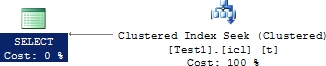
Figure 4-23. Execution plan with a clustered index
Table 't1'. Scan count 1, logical reads 2
![]() Note Even though a clustered index can outperform a nonclustered index in many instances of data retrieval, a table can have only one clustered index. Therefore, reserve the clustered index for a situation in which it can be of the greatest benefit.
Note Even though a clustered index can outperform a nonclustered index in many instances of data retrieval, a table can have only one clustered index. Therefore, reserve the clustered index for a situation in which it can be of the greatest benefit.
Benefits of a Nonclustered Index over a Clustered Index
As you learned in the previous section, a nonclustered index is preferred over a clustered index in the following situations:
- When the index key size is large
- To avoid the overhead cost associated with a clustered index since rebuilding the clustered index rebuilds all the nonclustered indexes of the table
- To resolve blocking by having a database reader work on the pages of a nonclustered index, while a database writer modifies other columns (not included in the nonclustered index) in the data page; in this case, the writer working on the data page won’t block a reader that can get all the required column values from the nonclustered index without hitting the base table. I’ll explain this in detail in Chapter 12.
- When all the columns (from a table) referred to by a query can be safely accommodated in the nonclustered index itself, as explained in this section
As already established, the data-retrieval performance when using a nonclustered index is generally poorer than that when using a clustered index, because of the cost associated with jumping from the nonclustered index rows to the data rows in the base table. In cases where the jump to the data rows is not required, the performance of a nonclustered index should be just as good as—or even better than—a clustered index. This is possible if the nonclustered index key includes all the columns required from the table.
To understand the situation in which a nonclustered index can outperform a clustered index, consider the following example. Assume for our purposes that you need to examine the credit cards that are expiring between the months of June and September of 2008. You may have a query that returns a large number of rows and looks like this:
SELECT cc.CreditCardID,
cc.CardNumber,
cc.ExpMonth,
cc.ExpYear
FROM Sales.CreditCard cc
WHERE cc.ExpMonth BETWEEN 6 AND 9
AND cc.ExpYear = 2008
ORDER BY cc.ExpMonth ;
The following are the I/O results, and Figure 4-24 shows the execution plan:
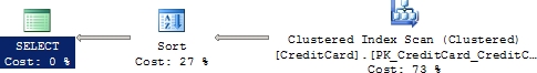
Figure 4-24. Execution plan scanning the clustered index
Table 'CreditCard'. Scan count 1, logical reads 189
The clustered index is on the primary key, and although most access against the table may be through that key, making the index useful, the cluster in this instance is just not performing in the way you need. Although you could expand the definition of the index to include all the other columns in the query, they’re not really needed to make the cluster function, and they would interfere with the operation of the primary key. Instead, you can use the INCLUDE operation to store the columns defined within it at the leaf level of the index. They don’t affect the key structure of the index in any way, but provide the ability, through the sacrifice of some additional disk space, to make a nonclustered index covering (covered in more detail later). In this instance, creating a different index is in order:
CREATE NONCLUSTERED INDEX ixTest
ON Sales.CreditCard (ExpMonth, ExpYear)
INCLUDE (CardNumber) ;
Now when the query is run again, this is the result:
Table 'CreditCard'. Scan count 1, logical reads 32
Figure 4-25 shows the corresponding execution plan.
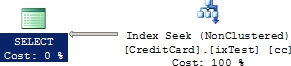
Figure 4-25. Execution plan with a nonclustered index
In this case, the SELECT statement doesn’t include any column that requires a jump from the nonclustered index page to the data page of the table, which is what usually makes a nonclustered index costlier than a clustered index for a large result set and/or sorted output. This kind of nonclustered index is called a covering index.
Clean up the index after the testing is done:
DROP INDEX Sales.CreditCard.ixTest ;
Advanced Indexing Techniques
A few of the more advanced indexing techniques that you can also consider are as follows:
- Covering indexes: These were introduced in the preceding section.
- Index intersections: Use multiple nonclustered indexes to satisfy all the column requirements (from a table) for a query.
- Index joins: Use the index intersection and covering index techniques to avoid hitting the base table.
- Filtered indexes: To be able to index fields with odd data distributions or sparse columns, a filter can be applied to an index so that it indexes only some data.
- Indexed views: This materializes the output of a view on disk.
- Index compression: The storage of indexes can be compressed through SQL Server, putting more rows of data on a page, improving performance.
- Columnstore indexes: Instead of grouping and storing data for a row, like traditional indexes, these indexes group and store based on columns.
I cover these topics in more detail in the following sections.
Covering Indexes
A covering index is a nonclustered index built upon all the columns required to satisfy a SQL query without going to the heap or the clustered index. If a query encounters an index and does not need to refer to the underlying structures at all, then the index can be considered a covering index.
For example, in the following SELECT statement, irrespective of where the columns are referred, all the columns (StateProvinceld and PostalCode) should be included in the nonclustered index to cover the query fully:
SELECT a.PostalCode
FROM Person.Address AS a
WHERE a.StateProvinceID = 42 ;
Then all the required data for the query can be obtained from the nonclustered index page, without accessing the data page. This helps SQL Server save logical and physical reads. If you run the query, you’ll get the following I/O and execution time as well as the execution plan in Figure 4-26.
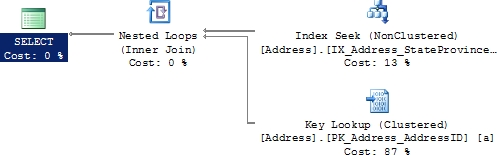
Figure 4-26. Query without a covering index
Table 'Address'. Scan count 1, logical reads 19.
Here you have a classic bookmark lookup with the Key Lookup operator pulling the PostalCode data from the clustered index and joining it with the Index Seek operator against the IX_Address_StateProvinceId index.
Although you can re-create the index with both key columns, another way to make an index a covering index is to use the new INCLUDE operator. This stores data with the index without changing the structure of the index itself. Use the following to re-create the index:
CREATE NONCLUSTERED INDEX [IX_Address_StateProvinceID]
ON [Person].[Address] ([StateProvinceID] ASC)
INCLUDE (PostalCode)
WITH (
DROP_EXISTING = ON) ;
If you rerun the query, the execution plan (Figure 4-27), I/O, and execution time change:
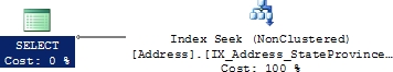
Figure 4-27. Query with a covering index
Table 'Address'. Scan count 1, logical reads 2
The reads have dropped from 19 to 2, and the execution plan is just about as simple as it’s possible to be; it’s a single Index Seek operation against the new and improved index, which is now covering. A covering index is a useful technique for reducing the number of logical reads of a query. Adding columns using the INCLUDE statement makes this functionality easier to achieve without adding to the number of columns in an index or the size of the index key since the included columns are stored only at the leaf level of the index.
The INCLUDE is best used in the following cases:
- You don’t want to increase the size of the index keys, but you still want to make the index a covering index.
- You’re indexing a data type that can’t be indexed (except text, ntext, and images).
- You’ve already exceeded the maximum number of key columns for an index (although this is a problem best avoided).
The covering index physically organizes the data of all the indexed columns in a sequential order. Thus, from a disk I/O perspective, a covering index that doesn’t use included columns becomes a clustered index for all queries satisfied completely by the columns in the covering index. If the result set of a query requires a sorted output, then the covering index can be used to physically maintain the column data in the same order as required by the result set— it can then be used in the same way as a clustered index for sorted output. As shown in the previous example, covering indexes can give better performance than clustered indexes for queries requesting a range of rows and/or sorted output. The included columns are not part of the key and therefore wouldn’t offer the same benefits for ordering as the key columns of the index.
To take advantage of covering indexes, be careful with the column list in SELECT statements to move only the data you need to. It’s also a good idea to use as few columns as possible to keep the index key size small for the covering indexes. Add columns using the INCLUDE statement in places where it makes sense. Since a covering index includes all columns used in a query, it has a tendency to be very wide, increasing the maintenance cost of the covering indexes. You must balance the maintenance cost with the performance gain that the covering index brings. If the number of bytes from all the columns in the index is small compared to the number of bytes in a single data row of that table and you are certain the query taking advantage of the covered index will be executed frequently, then it may be beneficial to use a covering index.
![]() Tip Covering indexes can also help resolve blocking and deadlocks, as you will see in Chapters 12 and 13.
Tip Covering indexes can also help resolve blocking and deadlocks, as you will see in Chapters 12 and 13.
Before building a lot of covering indexes, consider how SQL Server can effectively and automatically create covering indexes for queries on the fly using index intersection.
Index Intersections
If a table has multiple indexes, then SQL Server can use multiple indexes to execute a query. SQL Server can take advantage of multiple indexes, selecting small subsets of data based on each index and then performing an intersection of the two subsets (that is, returning only those rows that meet all the criteria). SQL Server can exploit multiple indexes on a table and then employ a join algorithm to obtain the index intersection between the two subsets.
In the following SELECT statement, for the WHERE clause columns, the table has a nonclustered index on the SalesPersonID column, but it has no index on the OrderDate column:
SELECT soh.*
FROM Sales.SalesOrderHeader AS soh
WHERE soh.SalesPersonID = 276
AND soh.OrderDate BETWEEN '4/1/2005' AND '7/1/2005' ;
Figure 4-28 shows the execution plan for this query.

Figure 4-28. Execution plan with no index on the OrderDate column
As you can see, the optimizer didn’t use the nonclustered index on the SalesPersonID column. Since the value of the OrderDate column is also required, the optimizer chose the clustered index to fetch the value of all the referred columns. The I/O for retrieving this data was as follows:
Table 'SalesOrderHeader'. Scan count 1, logical reads 686
To improve the performance of the query, the OrderDate column can be added to the nonclustered index on the SalesPersonId column or defined as an included column on the same index. But in this real-world scenario, you may have to consider the following while modifying an existing index:
- It may not be permissible to modify an existing index for various reasons.
- The existing nonclustered index key may be already quite wide.
- The cost of the queries using the existing index will be affected by the modification.
In such cases, you can create a new nonclustered index on the OrderDate column:
CREATE NONCLUSTERED INDEX IX_Test
ON Sales.SalesOrderHeader (OrderDate);
Run your SELECT command again.
Figure 4-29 shows the resultant execution plan of the SELECT statement.
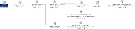
Figure 4-29. Execution plan with an index on the OrderDate column
As you can see, SQL Server exploited both the nonclustered indexes as index seeks (rather than scans) and then employed an intersection algorithm to obtain the index intersection of the two subsets. It then did a Key Lookup from the resulting dataset to retrieve the rest of the data not included in the indexes.
To improve the performance of a query, SQL Server can use multiple indexes on a table. Therefore, instead of creating wide index keys, consider creating multiple narrow indexes. SQL Server will be able to use them together where required, and when not required, queries benefit from narrow indexes. While creating a covering index, determine whether the width of the index will be acceptable and whether using include columns will get the job done. If not, then identify the existing nonclustered indexes that include most of the columns required by the covering index. You may already have two existing nonclustered indexes that jointly serve all the columns required by the covering index. If it is possible, rearrange the column order of the existing nonclustered indexes appropriately, allowing the optimizer to consider an index intersection between the two nonclustered indexes.
At times, it is possible that you may have to create a separate nonclustered index for the following reasons:
- Reordering the columns in one of the existing indexes is not allowed.
- Some of the columns required by the covering index may not be included in the existing nonclustered indexes.
- The total number of columns in the two existing nonclustered indexes may be more than the number of columns required by the covering index.
In such cases, you can create a nonclustered index on the remaining columns. If the combined column order of the new index and an existing nonclustered index meets the requirement of the covering index, the optimizer will be able to use index intersection. While identifying the columns and their order for the new index, try to maximize their benefit by keeping an eye on other queries, too.
Drop the index that was created for the tests:
DROP INDEX Sales.SalesOrderHeader.IX_Test;
Index Joins
The index join is a variation of index intersection, where the covering index technique is applied to the index intersection. If no single index covers a query but multiple indexes together can cover the query, SQL Server can use an index join to satisfy the query fully without going to the base table.
Let’s look at this indexing technique at work. Make a slight modification to the query from the “Index Intersections” section like this:
SELECT soh.SalesPersonID,
soh.OrderDate
FROM Sales.SalesOrderHeader AS soh
WHERE soh.SalesPersonID = 276
AND soh.OrderDate BETWEEN '4/1/2005' AND '7/1/2005' ;
The execution plan for this query is shown in Figure 4-30, and the reads are as follows:
Figure 4-30. Execution plan with no index join
Table 'SalesOrderHeader'. Scan count 1, logical reads 686
As shown in Figure 4-30, the optimizer didn’t use the existing nonclustered index on the SalesPersonID column. Since the query requires the value of the OrderDate column also, the optimizer selected the clustered index to retrieve values for all the columns referred to in the query. If an index is created on the OrderDate column like this:
CREATE NONCLUSTERED INDEX IX_Test
ON Sales.SalesOrderHeader (OrderDate ASC) ;
and the query is rerun, then Figure 4-31 shows the result, and you can see the reads here:
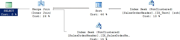
Figure 4-31. Execution plan with an index join
Table 'SalesOrderHeader'. Scan count 2, logical reads 4
The combination of the two indexes acts like a covering index reducing the reads against the table from 686 to 4 because it’s using two Index Seek operations joined together instead of a clustered index scan.
But what if the WHERE clause didn’t result in both indexes being used? Instead, you know that both indexes exist and that a seek against each would work like the previous query, so you choose to use an index hint:
SELECT soh.SalesPersonID
,soh.OrderDate FROM Sales.SalesOrderHeader AS soh WITH (INDEX (IX_Test,
IX_SalesOrderHeader_SalesPersonID)) WHERE soh.OrderDate BETWEEN '4/1/2002' AND '7/1/2002';
The results of this new query are shown in Figure 4-32, and the I/O is as follows:
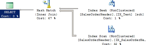
Figure 4-32. Execution plan with index join through a hint
able 'Worktable'. Scan count 0, logical reads 0
able 'SalesOrderHeader'. Scan count 2, logical reads 61
The reads have clearly increased, and you have a hash warning that tempdb was used to store data during the processing. Most of the time, the optimizer makes very good choices when it comes to indexes and execution plans. Although query hints are available to allow you to take control from the optimizer, this control can cause as many problems as it solves. In attempting to force an index join as a performance benefit, instead the forced selection of indexes slowed down the execution of the query.
Remove the test index before continuing:
DROP INDEX Sales.SalesOrderHeader.IX_Test ;
![]() Note While generating a query execution plan, the SQL Server optimizer goes through the optimization phases not only to determine the type of index and join strategy to be used but also to evaluate the advanced indexing techniques such as index intersection and index join. Therefore, instead of creating wide covering indexes, consider creating multiple narrow indexes. SQL Server can use them together to serve as a covering index yet use them separately where required. But you will need to test to be sure which works better in your situation, wider indexes,
Note While generating a query execution plan, the SQL Server optimizer goes through the optimization phases not only to determine the type of index and join strategy to be used but also to evaluate the advanced indexing techniques such as index intersection and index join. Therefore, instead of creating wide covering indexes, consider creating multiple narrow indexes. SQL Server can use them together to serve as a covering index yet use them separately where required. But you will need to test to be sure which works better in your situation, wider indexes,
or index intersections and joins.
A filtered index is a nonclustered index that uses a filter, basically a WHERE clause, to create a highly selective set of keys against a column or columns that may not have good selectivity otherwise. For example, a column with a large number of null values may be stored as a sparse column to reduce the overhead of those null values. Adding a filtered index to the column will allow you to have an index available on the data that is not null. The best way to understand this is to see it in action.
The Sales.SalesOrderHeader table has more than 30,000 rows. Of those rows, 27,000+ have a null value in the PurchaseOrderNumber column and the SalesPersonId column. If you wanted to get a simple list of purchase order numbers, the query might look like this:
SELECT soh.PurchaseOrderNumber,
soh.OrderDate,
soh.ShipDate,
soh.SalesPersonID
FROM Sales.SalesOrderHeader AS soh
WHERE PurchaseOrderNumber LIKE 'PO5%'
AND soh.SalesPersonID IS NOT NULL ;;
Running the query results in, as you might expect, a clustered index scan, and the following I/O and execution time, as shown in Figure 4-33.
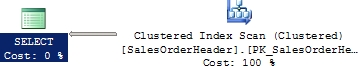
Figure 4-33. Execution plan without an index
Table 'SalesOrderHeader'. Scan count 1, logical reads 686
CPU time = 0 ms, elapsed time = 619 ms.
To fix this, it is possible to create an index and include some of the columns from the query to make this a covering index (as shown in Figure 4-34):
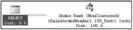
Figure 4-34. Execution plan with a covering index
CREATE NONCLUSTERED INDEX IX_Test
ON Sales.SalesOrderHeader(PurchaseOrderNumber ,SalesPersonID)
INCLUDE (OrderDate,ShipDate);
When you rerun the query, the performance improvement is fairly radical (see Figure 4-33 and the I/O and time in the following result):
Table 'SalesOrderHeader'. Scan count 1, logical reads 5 CPU time = 0 ms, elapsed time = 52 ms.
As you can see, the covering index dropped the reads from 686 down to 5 and the time from 619 ms to 52 ms. Normally, this would be enough. Assume for a moment that this query has to be called frequently—very frequently. Now, every bit of speed you can wring from it will pay dividends. Knowing that so much of the data in the indexed columns is null, you can adjust the index so that it filters out the null values, which aren’t used by the index anyway, reducing the size of the tree and therefore the amount of searching required:
CREATE NONCLUSTERED INDEX IX_Test
ON Sales.SalesOrderHeader(PurchaseOrderNumber,SalesPersonID)
INCLUDE (OrderDate,ShipDate)
WHERE PurchaseOrderNumber IS NOT NULL AND SalesPersonID IS NOT NULL
WITH (DROP_EXISTING = ON);
The final run of the query is visible in the following result and in Figure 4-35.
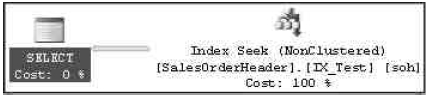
Figure 4-35. Execution plan with a filtered index
Table 'SalesOrderHeader'. Scan count 1, logical reads 4 CPU time = 0 ms, elapsed time = 40 ms.
Although in terms of sheer numbers reducing the reads from 5 to 4 isn’t much, it is a 20 percent reduction in the I/O cost of the query, and if this query were running hundreds or even thousands of times in a minute, as some queries do, that 20 percent reduction would be a great payoff indeed. Another visible evidence of the payoff is visible in the execution time, which dropped again from 52 ms to 40 ms.
Filtered indexes improve performance in many ways:
- Improving the efficiency of queries by reducing the size of the index
- Reducing storage costs by making smaller indexes
- Cutting down on the costs of index maintenance because of the reduced size
One of the first places suggested for their use is just like the previous example, eliminating null values from the index. You can also isolate frequently accessed sets of data with a special index so that the queries against that data perform much faster. You can use the WHERE clause to filter data in a fashion similar to creating an indexed view (covered in more detail in the “Indexed Views” section) without the data maintenance headaches associated with indexed views by creating a filtered index that is a covering index, just like the earlier example.
Filtered indexes require a specific set of ANSI settings when they are accessed or created:
- ON: ANSI_NULLS, ANSI_PADDING, ANSI_WARNINGS, ARITHABORT, CONCAT_NULL_YIELDS_NULL, QUOTED_IDENTIFIER
- OFF: NUMERIC_R0UNDAB0RT
When completed, drop the testing index:
DROP INDEX Sales.SalesOrderHeader.IX_Test;
Indexed Views
A database view in SQL Server is like a virtual table that represents the output of a SELECT statement. You create a view using the CREATE VIEW statement, and you can query it exactly like a table. In general, a view doesn’t store any data—only the SELECT statement associated with it. Every time a view is queried, it further queries the underlying tables by executing its associated SELECT statement.
A database view can be materialized on the disk by creating a unique clustered index on the view. Such a view is referred to as an indexed view or a materialized view. After a unique clustered index is created on the view, the view’s result set is materialized immediately and persisted in physical storage in the database, saving the overhead of performing costly operations during query execution. After the view is materialized, multiple nonclustered indexes can be created on the indexed view.
You can use an indexed view to increase the performance of a query in the following ways:
- Aggregations can be precomputed and stored in the indexed view to minimize expensive computations during query execution.
- Tables can be prejoined, and the resulting data set can be materialized.
- Combinations of joins or aggregations can be materialized.
Overhead
Indexed views can produce major overhead on an OLTP database. Some of the overheads of indexed views are as follows:
- Any change in the base table(s) has to be reflected in the indexed view by executing the view’s SELECT statement.
- Any changes to a base table on which an indexed view is defined may initiate one or more changes in the nonclustered indexes of the indexed view. The clustered index will also have to be changed if the clustering key is updated.
- The indexed view adds to the ongoing maintenance overhead of the database.
- Additional storage is required in the database.
The restrictions on creating an indexed view include the following:
- The first index on the view must be a unique clustered index.
- Nonclustered indexes on an indexed view can be created only after the unique clustered index is created.
- The view definition must be deterministic—that is, it is able to return only one possible result for a given query. (A list of deterministic and nondeterministic functions is provided in “SQL Server Books Online.”)
- The indexed view must reference only base tables in the same database, not other views.
- The indexed view may contain float columns. However, such columns cannot be included in the clustered index key.
- The indexed view must be a schema bound to the tables referred to in the view to prevent modifications of the table schema.
- There are several restrictions on the syntax of the view definition. (A list of the syntax limitations on the view definition is provided in “SQL Server Books Online.”)
- The list of SET options that must be fixed are as follows:
- ON: ARITHABORT, CONCAT_NULL_YIELDS_NULL, QUOTED_IDENTIFIER, ANSI_NULLS, ANSI_ PADDING, and ANSI_WARNING
- OFF: NUMERIC_ROUNDABORT
![]() Note If the query connection settings don’t match these ANSI standard settings, you may see errors on the insert/update/delete of tables that are used within the indexed view.
Note If the query connection settings don’t match these ANSI standard settings, you may see errors on the insert/update/delete of tables that are used within the indexed view.
Usage Scenarios
Reporting systems benefit the most from indexed views. OLTP systems with frequent writes may not be able to take advantage of the indexed views because of the increased maintenance cost associated with updating both the view and the underlying base tables. The net performance improvement provided by an indexed view is the difference between the total query execution savings offered by the view and the cost of storing and maintaining the view.
An indexed view need not be referenced in the query for the query optimizer to use it during query execution. This allows existing applications to benefit from the newly created indexed views without changing those applications. The query optimizer considers indexed views only for queries with nontrivial cost. You may also find that the new columnstore index will work better for you than indexed views, especially when you’re preaggregating data.
Let’s see how indexed views work with the following example. Consider the three queries in Listings 4-1 through 4-3.
SELECT p.[Name] AS ProductName,
SUM(pod.OrderQty) AS OrderOty,
SUM(pod.ReceivedQty) AS ReceivedOty,
SUM(pod.RejectedQty) AS RejectedOty
FROM Purchasing.PurchaseOrderDetail AS pod
JOIN Production.Product AS p
ON p.ProductID = pod.ProductID
GROUP BY p.[Name] ;
Listing 4-2. Query2.sql
SELECT p.[Name] AS ProductName,
SUM(pod.OrderQty) AS OrderOty,
SUM(pod.ReceivedQty) AS ReceivedOty,
SUM(pod.RejectedQty) AS RejectedOty
FROM Purchasing.PurchaseOrderDetail AS pod
JOIN Production.Product AS p
ON p.ProductID = pod.ProductID
GROUP BY p.[Name]
HAVING (SUM(pod.RejectedQty) / SUM(pod.ReceivedQty)) > .08;
SELECT p.[Name] AS ProductName,
SUM(pod.OrderQty) AS OrderQty,
SUM(pod.ReceivedQty) AS ReceivedQty,
SUM(pod.RejectedQty) AS RejectedQty
FROM Purchasing.PurchaseOrderDetail AS pod
JOIN Production.Product AS p
ON p.ProductID = pod.ProductID
WHERE p.[Name] LIKE ‘Chain%'
GROUP BY p.[Name] ;
All three queries use the aggregation function SUM on columns of the PurchaseOrderDetail table. Therefore, you can create an indexed view to precompute these aggregations and minimize the cost of these complex computations during query execution.
Listings 4-4 through 4-6 show the number of logical reads performed by these queries to access the appropriate tables.
Listing 4-4. Logical Reads by Query1
Table 'Worktable'. Scan count 0, logical reads 0
Table 'Product'. Scan count 1, logical reads 6
Table 'PurchaseOrderDetail'. Scan count 1, logical reads 66
CPU time = 0 ms, elapsed time = 33 ms.CPU time = 15 ms, elapsed time = 100 ms.
Listing 4-5. Logical Reads by Query2
Table 'Worktable'. Scan count 0, logical reads 0
Table 'Product'. Scan count 1, logical reads 6
Table 'PurchaseOrderDetail'. Scan count 1, logical reads 66CPU time = 16 ms,
elapsed time = 12 ms.
Listing 4-6. Logical Reads by Query3
Table 'PurchaseOrderDetail'. Scan count 5, logical reads 894
Table 'Product'. Scan count 1, logical reads 2
CPU time = 16 ms, elapsed time = 5 ms.
Create an indexed view to precompute the costly computations and join the tables (odView.sql in the download):
IF EXISTS ( SELECT *
FROM sys.views
WHERE object_id = OBJECT_ID(N'[Purchasing].[IndexedView]') )
DROP VIEW [Purchasing].[IndexedView] ;
GO
CREATE VIEW Purchasing.IndexedView
WITH SCHEMABINDING
AS
SELECT pod.ProductID,
SUM(pod.OrderQty) AS OrderQty,
SUM(pod.ReceivedQty) AS ReceivedQty,
SUM(pod.RejectedQty) AS RejectedQty,
COUNT_BIG(*) AS [Count]
FROM Purchasing.PurchaseOrderDetail AS pod
GROUP BY pod.ProductID ;
GO
CREATE UNIQUE CLUSTERED INDEX iv
ON Purchasing.IndexedView (ProductID) ;
GO
Certain constructs such as AVG are disallowed. (For the complete list of disallowed constructs, refer to “SQL Server Books Online.”) If aggregates are included in the view, as in this one, you must include COUNT_BIG by default.
The indexed view materializes the output of the aggregate functions on the disk. This eliminates the need for computing the aggregate functions during the execution of a query interested in the aggregate outputs. For example, Query3.sql requests the sum of ReceivedQty and RejectedQty for certain products from the PurchaseOrderDetail table. Because these values are materialized in the indexed view for every product in the PurchaseOrderDetail table, you can fetch these preaggregated values using the following SELECT statement on the indexed view:
SELECT iv.ProductID,
iv.ReceivedQty,
iv.RejectedQty
FROM Purchasing.IndexedView AS iv ;
As shown in the execution plan in Figure 4-36, the SELECT statement retrieves the values directly from the indexed view without accessing the base table (PurchaseOrderDetail).
Figure 4-36. Execution plan with an indexed view
The indexed view benefits not only the queries based on the view directly but also other queries that may be interested in the materialized data. For example, with the indexed view in place, the three queries on PurchaseOrderDetail benefit without being rewritten (see the execution plan in Figure 4-37 for the execution plan from the first query), and the number of logical reads decreases, as shown in Listings 4-7 through 4-9.
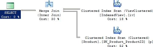
Figure 4-37. Execution plan with the indexed view automatically used
Listing 4-7. Logical Reads by Query1 with an Indexed View
Table 'Product'. Scan count 1, logical reads 13
Table 'IndexedView'. Scan count 1, logical reads 4
CPU time = 0 ms, elapsed time = 99 ms.
Listing 4-8. Logical Reads by Query2 with an Indexed View
Table 'Product'. Scan count 1, logical reads 13
Table 'IndexedView'. Scan count 1, logical reads 4
CPU time = 0 ms, elapsed time = 28 ms.
Listing 4-9. Logical Reads by Query3 with an Indexed View
Table 'IndexedView'. Scan count 0, logical reads 10
Table 'Product'. Scan count 1, logical reads 2
CPU time = 0 ms, elapsed time = 35 ms.
Even though the queries are not modified to refer to the new indexed view, the optimizer still uses the indexed view to improve performance. Thus, even existing queries in the database application can benefit from new indexed views without any modifications to the queries. If you do need different aggregations than what the indexed view offers, you’ll be out of luck. Here again the columnstore index shines.
Index Compression
Data and index compression was introduced in SQL Server 2008 (available in the Enterprise and Developer Editions). Compressing an index means getting more key information onto a single page. This can lead to significant performance improvements because fewer pages and fewer index levels are needed to store the index. There will be overhead in the CPU as the key values in the index are compressed and decompressed, so this may not be a solution for all indexes. Memory benefits also because the compressed pages are stored in memory in a compressed state.
By default, an index will be not be compressed. You have to explicitly call for the index to be compressed when you create the index. There are two types of compression: row- and page-level compression. Nonleaf pages in an index receive no compression under the page type. To see index compression in action, consider the following index (don’t run this code since the index already exists):
CREATE NONCLUSTERED INDEX IX_Test
ON Person.Address(City ASC, PostalCode ASC) ;
This index was created earlier in the chapter. If you were to re-create it as defined here, this creates a row type of compression on an index with the same two columns as the first test index IX_Test.
CREATE NONCLUSTERED INDEX IX_Comp_Test
ON Person.Address (City,PostalCode)
WITH (DATA_COMPRESSION = ROW ) ;
Create one more index:
CREATE NONCLUSTERED INDEX IX_Comp_Page_Test
ON Person.Address (City,PostalCode)
WITH (DATA_COMPRESSION = PAGE) ;
To examine the indexes being stored, modify the original query against sys.dm_db_index_ physical_stats to add another column, compressed_page_count:
SELECT i.Name,
i.type_desc,
s.page_count,
s.record_count,
s.index_level,
compressed_page_count
FROM sys.indexes i
JOIN sys.dm_db_index_physical_stats(DB_ID(N'AdventureWorks2008R2'),
OBJECT_ID(N'Person.Address'), NULL,
NULL, 'DETAILED') AS s
ON i.index_id = s.index_id
WHERE i.OBJECT_ID = OBJECT_ID(N'Person.Address') ;
Running the query, you get the results in Figure 4-38.

Figure 4-38. sys.dm_db_index_physical_stats output about compressed indexes
For this index, you can see that the page compression was able move the index from 106 pages down to 25, of which 25 were compressed. The row type compression in this instance made a difference in the number of pages in the index, but not nearly as dramatic as that of the page compression.
To see the compression in action, run the following query:
SELECT a.City,
a.PostalCode
FROM Person.Address AS a
WHERE a.City = 'Newton'
AND a.PostalCode = 'V2M1N7' ;
The optimizer chose, on my system, to use the IXCompPageTest index. Even if I forced it to use the IXTest index, thusly, the performance was identical, although one extra page was read in the second query.
SELECT a.City,
a.PostalCode
FROM Person.Address AS a WITH (INDEX = IX_Test)
WHERE a.City = 'Newton'
AND a.PostalCode = 'V2M1N7' ;
So although one index is taking up radically less room on approximately one quarter as many pages, it’s done at no cost in performance.
Compression has a series of impacts on other processes within SQL Server, so further understanding of the possible impacts as well as the possible benefits should be explored thoroughly prior to implementation. In most cases, the cost to CPU is completely outweighed by the benefits everywhere else, but you should test and monitor your system.
Clean up the indexes after you finish testing:
DROP INDEX Person.Address.IX_Test;
DROP INDEX Person.Address.IX_Comp_Test;
DROP INDEX Person.Address.IX_Comp_Page_Test;
Introduced in SQL Server 2012, the columnstore index is used to index information by columns rather than by rows. This is especially useful when working within data warehousing systems where very large amounts of data have to be aggregated and accessed quickly. The information stored within a columnstore index is grouped on each column, and these groupings are stored individually. This makes aggregations on different sets of columns extremely fast since the columnstore index can be accessed rather than accessing large numbers of rows in order to aggregate the information and because the columnar data is stored compressed. There are a number of limits on using columnstore indexes:
- Tables that have a columnstore index cannot be updated. You must first drop the columnstore index or you must partition around the columnstore index in order to support changes to the underlying data.
- You can’t use certain data types such as binary, text, varchar(max), uniqueidentifier, clr data types, xml, or decimal with a precision greater than 18.
- You can’t create a columnstore index on a sparse column.
For the complete list of restrictions, refer to “Books Online.”
Columnstores are primarily meant for use within data warehouses and therefore work best when dealing with the associated styles of storage such as star schemas. You can see how a columnstore can help even with OLTP systems if you can isolate the storage so that updates are controlled. In the AdventureWorks2008R2 database, the Production.TransactionHistoryArchive table is a structure that is more likely to be used for aggregate queries than many of the other structures. Since it’s an archive table, the load of it is also controlled so that a columnstore index could be used successfully here. Take this query as an example:
SELECT tha.ProductID,
COUNT(tha.ProductID) AS CountProductID,
SUM(tha.Quantity) AS SumQuantity,
AVG(tha.ActualCost) AS AvgActualCost
FROM Production.TransactionHistoryArchive AS tha
GROUP BY tha.ProductID ;
If you run this query against the table as it is currently configured, you’ll see an execution plan that looks like Figure 4-39.
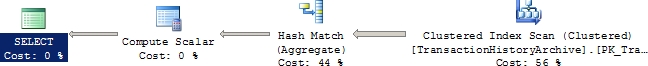
Figure 4-39. A clustered index scan and hash match aggregate for a GROUP BY query
The reads and execution time for the query are as follows:
Table 'Worktable'. Scan count 0, logical reads 0
Table 'TransactionHistoryArchive'. Scan count 1, logical reads 622
CPU time = 94 ms, elapsed time = 348 ms.
There are a large number of reads, and this query uses quite a bit of CPU and is not terribly fast to execute. Creating a columnstore index is very simple:
CREATE NONCLUSTERED COLUMNSTORE INDEX ix_csTest
ON Production.TransactionHistoryArchive
(ProductID,
Quantity,
ActualCost) ;
With the columnstore index in place, the optimizer now has the option of using that index to satisfy the foregoing query. Just like all other indexes available to the optimizer, costs are associated with the columnstore index, so it may or may not be chosen to satisfy the requirements for any given query against the table. In this case, if you rerun the original aggregate query, you can see that the optimizer determined that the costs associated with using the columnstore index were beneficial to the query. The execution plan now looks like Figure 4-40.
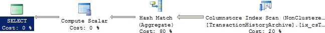
Figure 4-40. The columnstore index is used instead of the clustered index.
As you can see, the basic operations of the query are the same, but the columnstore index is scanned instead of the clustered index. The real differences are seen in the reads and execution times for the query:
Table 'Worktable'. Scan count 0, logical reads 0
Table 'TransactionHistoryArchive'. Scan count 1, logical reads 54
CPU time = 78 ms, elapsed time = 194 ms.
The radical reduction in the number of reads required to retrieve the data and the marginal increase in speed are all the result of being able to reference information that is indexed by column instead of by row. The foregoing query ran in what’s called row mode. A columnstore index has two operations, batch mode and row mode.
Of the two, batch mode is much faster. It takes advantage of a special method of accessing the data that allows for pulling large sets of data, in batches, so that decompression isn’t necessary. The batch mode processing also has extra benefits when working with multiprocessor machines. To see if a columnstore ran in batch or row mode, you just have to check the properties of the columnstore operation. For example, in the foregoing query, here’s the property sheet from the columnstore scan operator in Figure 4-41.
Figure 4-41. Actual execution mode
There is only a limited set of operations, documented in “Books Online,” that result in batch mode processing, but when working with those operations on a system with enough processors, you will see yet another substantial performance enhancement.
Columnstore indexes don’t require you to have the columns in a particular order, unlike clustered and nonclustered indexes. Also, unlike these other indexes, you should place multiple columns within a columnstore index so that you get benefits across those columns. But if you’re retrieving large numbers of columns from a columnstore index, you might see some performance degradation.
While the limitations for the use of the columnstore index are stringent, the benefits for structures that can operate within those limitations are very clear.
Special Index Types
As special data types and storage mechanisms are introduced to SQL Server by Microsoft, methods for indexing these special storage types are also developed. Explaining all the details possible for each of these special index types is outside the scope of the book. In the following sections, I introduce the basic concepts of each index type in order to facilitate the possibility of their use in tuning your queries.
You can store large amounts of text in SQL Server by using the MAX value in the VARCHAR, NVARCHAR, CHAR, and NCHAR fields. A normal clustered or nonclustered index against these large fields would be unsupportable because a single value can far exceed the page size within an index. So, a different mechanism of indexing text is to use the full-text engine, which must be running to work with full-text indexes. You can also build a full-text index on VARBINARY data.
You need to have one column on the table that is unique. The best candidates for performance are integers: INT or BIGINT. This column is then used along with the word to identify which row within the table it belongs to, as well as its location within the field. SQL Server allows for incremental changes, either change tracking or time-based, to the full-text indexes as well as complete rebuilds.
SQL Server 2012 introduces another method for working with text called Semantic Search. It uses phrases from documents to identify relationships between different sets of text stored within the database.
Introduced in SQL Server 2008 is the ability to store spatial data. This data can be either a geometry type or the very complex geographical type, literally identifying a point on the earth. To say the least, indexing this type of data is complicated. SQL Server stores these indexes in a flat B-tree, similar to regular indexes, except that it is also a hierarchy of four grids linked together. Each of the grids can be given a density of low, medium, or high, outlining how big each grid is. There are mechanisms to support indexing of the spatial data types so that different types of queries, such as finding when one object is within the boundaries or near another object, can benefit from performance increases inherent in indexing.
A spatial index can be created only against a column of type geometry or geography. It has to be on a base table, it must have no indexed views, and the table must have a primary key. You can create up to 249 spatial indexes on any given column on a table. Different indexes are used to define different types of index behavior. More information is available in the book Beginning Spatial with SQL Server 2008 by Alastair Aitchison (Apress, 2009).
Introduced as a data type in SQL Server 2005, XML can be stored not as text but as well-formed XML data within SQL Server. This data can be queried using the XQuery language as supported by SQL Server. To enhance the performance capabilities, a special set of indexes has been defined. An XML column can have one primary and several secondary indexes. The primary XML shreds the properties, attributes, and elements of the XML data and stores it as an internal table. There must be a primary key on the table, and that primary key must be clustered in order to create an XML index. After the XML index is created, the secondary indexes can be created. These indexes have types Path, Value, and Property, depending on how you query the XML. For more details, check out Pro SQL Server 2008 XML by Michael Coles (Apress, 2008).
Additional Characteristics of Indexes
Other index properties can affect performance, positively and negatively. A few of these behaviors are explored here.
SQL Server supports creating a composite index with a different sort order for the different columns of the index. Suppose you want an index with the first column sorted in ascending order and the second column sorted in descending order in order to eliminate a sort operation, which can be quite costly. You could achieve this as follows:
CREATE NONCLUSTERED INDEX i1 ON t1(c1 ASC, c2 DESC) ;
Index on Computed Columns
You can create an index on a computed column, as long as the expression defined for the computed column meets certain restrictions, such as that it references columns only from the table containing the computed column and it is deterministic.
Index on BIT Data Type Columns
SQL Server allows you to create an index on columns with the BIT data type. The ability to create an index on a BIT data type column by itself is not a big advantage since such a column can have only two unique values, except for the rare circumstance where the vast majority of the data is one value and only a few rows are the other. As mentioned previously, columns with such low selectivity (number of unique values) are not usually good candidates for indexing. However, this feature comes into its own when you consider covering indexes. Because covering indexes require including all the columns in the index, the ability to add the BIT data type column to an index allows covering indexes to include such a column, if required.
CREATE INDEX Statement Processed As a Query
The CREATE INDEX operation is integrated into the query processor. The optimizer can use existing index(es) to reduce scan cost and sort while creating an index.
Take, for example, the Person.Address table. A nonclustered index exists on a number of columns: AddressLine1, AddressLine2, City, StateProvinceld, and PostalCode. If you needed to run queries against the City column with the existing index, you’ll get a scan of that index. Now create a new index like this:
CREATE INDEX IX_Test
ON Person.Address(City) ;
You can see in Figure 4-42 that, instead of scanning the table, the optimizer chose to scan the index in order to create the new index because the column needed for the new index was contained within the other nonclustered index.

Figure 4-42. Execution plan for CREATE INDEX
SQL Server supports parallel plans for a CREATE INDEX statement, as supported in other SQL queries. On a multiprocessor machine, index creation won’t be restricted to a single processor but will benefit from the multiple processors. You can control the number of processors to be used in a CREATE INDEX statement with the max degree of parallelism configuration parameter of SQL Server. The default value for this parameter is 0, as you can see by executing the sp_configure stored procedure:
EXEC sp_configure
'max degree of parallelism' ;
The default value of 0 means that SQL Server can use all the available CPUs in the system for the parallel execution of a T-SQL statement. On a system with four processors, the maximum degree of parallelism can be set to 2 by executing spconfigure:
EXEC sp_configure
'max degree of parallelism',
2 ;
RECONFIGURE WITH OVERRIDE ;
This allows SQL Server to use up to two CPUs for the parallel execution of a T-SQL statement. This configuration setting takes effect immediately, without a server restart.
The query hint MAXDOP can be used for the CREATE INDEX statement. Also, be aware that the parallel CREATE INDEX feature is available only in SQL Server Enterprise Editions.
The default creation of an index is done as an offline operation. This means that exclusive locks are placed on the table, restricting user access while the index is created. It is possible to create the indexes as an online operation. This allows users to continue to access the data while the index is being created. This comes at the cost of increasing the amount of time and resources it takes to create the index. With SQL Server 2012, indexes with varchar(MAX), nvarchar(MAX), and nbinary(MAX) can actually be rebuilt online. Online index operations are available only in SQL Server Enterprise Editions.
Considering the Database Engine Tuning Advisor
A simple approach to indexing is to use the Database Engine Tuning Advisor tool provided by SQL Server. This tool is a usage-based tool that looks at a particular workload and works with the query optimizer to determine the costs associated with various index combinations. Based on the tool’s analysis, you can add or drop indexes as appropriate.
![]() Note I will cover the Database Engine Tuning Advisor tool in more depth in Chapter 5.
Note I will cover the Database Engine Tuning Advisor tool in more depth in Chapter 5.
Summary
In this chapter, you learned that indexing is an effective method for reducing the number of logical reads and disk I/O for a query. Although an index may add overhead to action queries, even action queries such as UPDATE and DELETE can benefit from an index.
To decide the index key columns for a particular query, evaluate the WHERE clause and the join criteria of the query. Factors such as column selectivity, width, data type, and column order are important in deciding the columns in an index key. Since an index is mainly useful in retrieving a small number of rows, the selectivity of an indexed column should be very high. It is important to note that nonclustered indexes contain the value of a clustered index key as their row locator, because this behavior greatly influences the selection of an index type.
For better performance, try to cover a query fully using a covering index. Since SQL Server can benefit from multiple indexes, use the index intersection and index join techniques, and consider having multiple narrow indexes instead of one very wide index. When working with special data types, apply the indexes that work with those special data types in order to help performance.
In the next chapter, you will learn more about the Database Engine Tuning Advisor, the SQL Server–provided tool that can help you determine the correct indexes in a database for a given SQL workload.