Chapter 3
![]()
SQL Query Performance Analysis
A common cause of slow SQL Server performance is a heavy database application workload—the nature of the queries themselves. Thus, to analyze the cause of a system bottleneck, it is important to examine the database application workload and identify the SQL queries causing the most stress on system resources. To do this, you can use the Extended Events and other Management Studio tools.
In this chapter, I cover the following topics:
- The basics of the Extended Events
- How to analyze SQL Server workload and identify costly SQL queries using Extended Events
- How to combine the baseline measurements with data collected from Extended Events
- How to analyze the processing strategy of a costly SQL query using Management Studio
- How to track query performance through dynamic management objects
- How to analyze the effectiveness of index and join strategies for a SQL query
- How to measure the cost of a SQL query using SQL utilities
Extended Events were introduced in SQL Server 2008, but with no GUI in place and a reasonably complex set of code to set them up, they weren’t used much to capture performance metrics. With SQL Server 2012, a GUI for managing extended events was introduced, making this the preferred mechanism for gathering query performance metrics among other things. The SQL Profiler and traces, previously the best mechanism for gathering these metrics is going into deprecation. It’s still available, but it’s on its way out. As a result, all examples in the book will be using extended events.
The Extended Events wizard allows you to do the following:
- Graphically monitor SQL Server queries
- Collect query information in the background
- Analyze performance
- Diagnose problems such as deadlocks
- Debug a Transact-SQL (T-SQL) statement
You can also use Extended events to capture other sorts of activities performed on a SQL Server instance. You can run extended events from the graphical front end or through direct calls to the procedures. The most efficient way to define a trace is through the system procedures, but a good place to start learning about sessions is through the GUI.
Extended Events Sessions
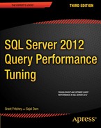
Extended Events are found in the Management Studio GUI. You can navigate through the Object Explorer to the Management folder on a given instance to find the Extended Events folder. From there you can look at Sessions that have already been built on the system, but to start setting up your own sessions, just right-click the Sessions folder and select “New Session Wizard.” An introduction screen will open the first time you run the wizard. You can turn it off so that it stops displaying. The next screen is the “Set Session Properties” screen as shown in Figure 3.1:
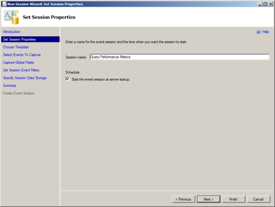
Figure 3.1. Extended Events New Session Wizard, the first screen.
You will have to supply a Session Name. I strongly suggest giving it a very clear name so you know what the session is doing when you check on it later. Whether or not you set the session to start with the server is a different decision that you’ll have to make on your own. Collecting performance metrics over a long period of time generates lots of data that you’ll have to deal with. Clicking the Next button will open the Choose Template screen as shown in Figure 3-2:
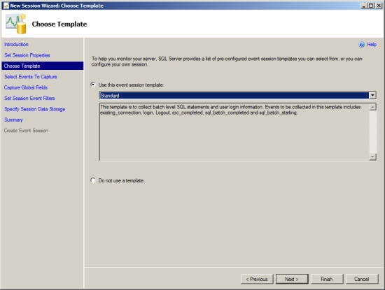
Figure 3-2. Extended Events New Session Wizard, Choose Template screen
Multiple templates are available and you can use those as a basis for your own Sessions. Eventually you’ll find that you need to build your own sessions from scratch and ultimately you’ll simply use the TSQL commands to build out your sessions. For this example I’ll go ahead and use the Standard template, which basically identical to the old Standard template in the deprecated Profiler GUI. Clicking the Next button will take us to the Select Events To Capture window.
An event represents various activities performed in SQL Server and in some cases, the underlying operating system. There’s an entire architecture around event targets, event packages and event sessions, but the use of the GUI means you don’t have to worry about all that. We will cover some of the architecture when we script a session later in this chapter. Figure 3-3 shows the events that are defined by the Standard template:
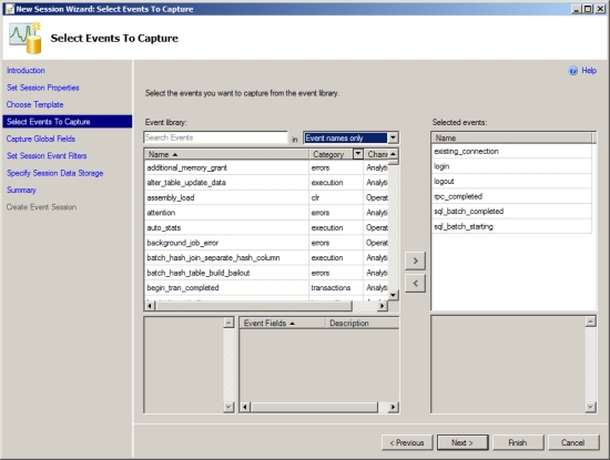
Figure 3-3. Extended Events Wizard, Select Events to Capture window
For performance analysis, you are mainly interested in the events that help you judge levels of resource stress for various activities performed on SQL Server. By resource stress, I mean things such as the following:
- What kind of CPU utilization was involved for the SQL activity?
- How much memory was used?
- How much I/O was involved?
- How long did the SQL activity take to execute?
- How frequently was a particular query executed?
- What kind of errors and warnings were faced by the queries?
You can calculate the resource stress of a SQL activity after the completion of an event, so the main events you use for performance analysis are those that represent the completion of a SQL activity. Table 3-1 describes these events.
Table 3-1. Events toMonitor Query Completion
| Event Category | Event | Description |
| Execution | rpc_completed | A remote procedure call completion event |
| sp_statement_completed | A SQL statement completion event within a stored procedure | |
| sql_batch_completed | A T-SQL batch completion event | |
| sql_statement_completed | A T-SQL statement completion event |
An RPC event indicates that the stored procedure was executed using the Remote Procedure Call (RPC) mechanism through an OLEDB command. If a database application executes a stored procedure using the T-SQL EXECUTE statement, then that stored procedure is resolved as a SQL batch rather than as an RPC.
A T-SQL batch is a set of SQL queries that are submitted together to SQL Server. A T-SQL batch is usually terminated by a GO command. The GO command is not a T-SQL statement. Instead, the GO command is recognized by the sqlcmd utility, as well as by Management Studio, and it signals the end of a batch. Each SQL query in the batch is considered a T-SQL statement. Thus, a T-SQL batch consists of one or more T-SQL statements. Statements or T-SQL statements are also the individual, discrete commands within a stored procedure. Capturing individual statements with the sp_statement_completed or sql_statement_completed event can be a more expensive operation, depending on the number of individual statements within your queries. Assume for a moment that each stored procedure within your system contains one, and only one, T-SQL statement.
In this case, the collection of completed statements is very low. Now assume that you have multiple statements within your procedures and that some of those procedures are calls to other procedures with other statements. Collecting all this extra data now becomes a more noticeable load on the system. My own testing suggested that you won’t see much impact until you’re hitting upward of ten distinct statements per procedure. Statement completion events should be collected judiciously, especially on a production system. You should apply filters to limit the returns from these events. Filters are covered later in this chapter.
After you’ve selected a trace template, a preselected list of events will already be defined in the Selected Events list on the right. To add an event to the session, find the event in the Event library and use the arrow buttons to move the event from the library to the Selected Events list. To remove events not required, click the arrow to move it back out of the list and into the library.
Although the events listed in Table 3-1 represent the most common events used for determining query performance, you can sometimes use a number of additional events to diagnose the same thing. For example, as mentioned in Chapter 1, repeated recompilation of a stored procedure adds processing overhead, which hurts the performance of the database request. The execution category in the Event library includes an event, sql_statement_recompile, to indicate the recompilation of a statement (this event is explained in depth in Chapter 10). The Event library contains additional events to indicate other performance-related issues with a database workload. Table 3-2 shows a few of these events.
Table 3-2. Events for Query Performance
| Event Category | Event | Description |
| Session | login logout |
Keeps track of database connections when users connect to and disconnect from SQL Server. |
| existing_connection | Represents all the users connected to SQL Server before the session was started. | |
| cursor | cursor_implicit_ conversion |
Indicates that the cursor type created is different from the requested type. |
| errors | attention | Represents the intermediate termination of a request caused by actions such as query cancellation by a client or a broken database connection including timeouts. |
| error_reported | Occurs when an error is reported. | |
| execution_warning | Indicates the occurrence of any warning during the execution of a query or a stored procedure. | |
| hash_warning | Indicates the occurrence of an error in a hashing operation. | |
| warnings | missing_column_statistics | Indicates that the statistics of a column, statistics required by the optimizer to decide a processing strategy, are missing. |
| missing_join_predicate | Indicates that a query is executed with no joining predicate between two tables. | |
| sort_warnings | Indicates that a sort operation performed in a query such as SELECT did not fit into memory. | |
| lock | lock_deadlock | Occurs when a process is chosen as a deadlock victim |
| lock_deadlock_chain | Shows a trace of the chain of queries creating the deadlock. | |
| lock_timeout | Signifies that the lock has exceeded the timeout parameter, which is set by SET LOCK_TIMEOUT timeout_period(ms). | |
| execution | sql_statement_recompile | Indicates that an execution plan for a query statement had to be recompiled, because one did not exist, a recompilation was forced, or the existing execution plan could not be reused. |
| rpc_starting | Represents the starting of a stored procedure. They are useful to identify procedures that started but could not finish because of an operation that caused an Attention event. | |
| Query_post_compilation_ showplan |
Shows the execution plan after a SQL statement has been compiled. | |
| Query_post_execution_ showplan |
Shows the execution plan after the SQL statement has been executed which includes execution statistics | |
| transactions | sql_transaction | Provides information about a database transaction, including information such as when a transaction starts, completes, and rolls back |
Once you’ve selected the events that are of interest in the Session Wizard, you’ll have to click next, which will open the Capture Global Fields window as shown in Figure 3-4:
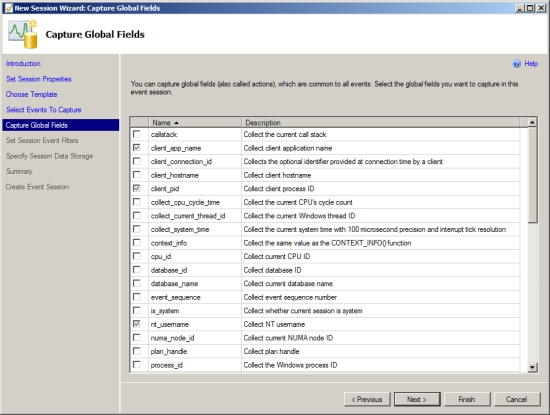
Figure 3-4. Capture Global Fields screen allows you to select Fields or Actions for the Events you’re monitoring
The fields, called actions in the TSQL, represent different attributes of an event, such as the user involved with the event, the SQL statement for the event, the resource cost of the event, and the source of the event.
The standard set of event fields are generated by the wizard and the template, others are automatic with the event type. You can select others from the list in the wizard. Table 3-3 shows some of the common actions that you’ll use for performance analysis.
Table 3-3. Actions Command for Query Analysis
| Data Column | Description |
| Statement | The SQL text from the rpc_completed event |
| Batch_text | The SQL text from the sql_batch_completed event |
| cpu_time | CPU cost of an event in microseconds (mc). For example, CPU = 100 for a SELECT statement indicates that the statement took 100 mc to execute. |
| logical_reads | Number of logical reads performed for an event. For example, logical_reads = 800 for a SELECT statement indicates that the statement required a total of 800 page reads. |
| Physical_reads | Number of physical reads performed for an event, can differ from the logical_reads due to access to the disk subsystem |
| writes | Number of logical writes performed for an event. |
| duration | Execution time of an event in ms. |
| session_id | SQL Server session identifier used for the event. |
Each logical read and write consists of an 8KB page activity in memory, which may require zero or more physical I/O operations.
To add an action, just click the check box in the list provided in the Global Fields page shown in
Figure 3-4. You can use additional data columns from time to time to diagnose the cause of poor performance. For example, in the case of a stored procedure recompilation, the event indicates the cause of the recompile through the recompile_cause event field (This field is explained in depth in Chapter 10.) A few of the commonly used additional actions are as follows:
- plan_handle
- query_hash
- query_plan_hash
- database_id
- client_app_name
- transaction_id
Other information is available as part of the event fields. For example the binary_data and integer_data event fields provide specific information about a given SQL Server activity. For example, in the case of a cursor, they specify the type of cursor requested and the type of cursor created. Although the names of these additional fields indicate their purpose to a great extent, I will explain the usefulness of these global fields in later chapters as you use them.
In addition to defining events and fields for an extended event session, you can also define various filter criteria. These help keep the session output small, which is usually a good idea. Table 3-4 describes the filter criteria that you will commonly use during performance analysis.
| Events | Filter Criteria Example | Use |
| sqlserver.username | = <some value> | Captures only events for a single user or login |
| sqlserver.database_id | = <ID of the database to monitor> |
This filters out events generated by other databases. You can determine the ID of a database from its name as follows: SELECT DB_ID('AdventureWorks2008R2'). |
| sqlos.duration | >= 200 | For performance analysis, you will often capture a trace for a large workload. In a large trace, there will be many event logs with a duration that is less than what you're interested in. Filter out these event logs, because there is hardly any scope for optimizing these SQL activities. |
| sqlserver.physical_ reads |
>= 2 | This is similar to the criterion on the duration filter. |
| sqlserver.session_id | = <Database users to monitor> |
This troubleshoots queries sent by a specific server session |
Figure 3-4 shows a snippet of the preceding filter criteria selection in the Session Wizard.
If you look at the Field value in Figure 3-5, you’ll note that it says sqlserver.database_id. This is because there are different sets of data available to you and they are qualified by the type of data being referenced. In this case, we’re talking specifically about a sqlserver.database_id. But we could be referring to something from the sqlos or even the Extended Events package itself.
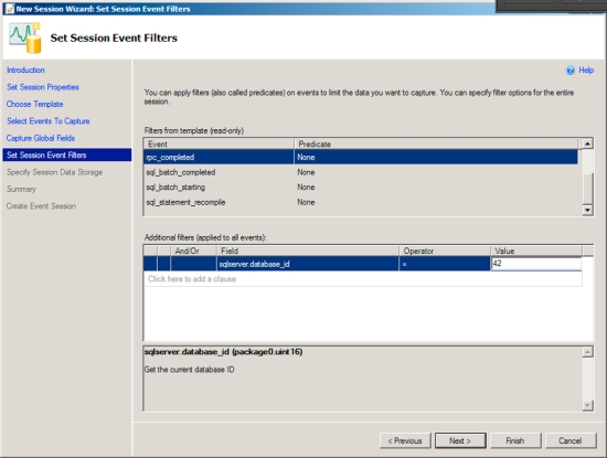
Figure 3-5. Filters applied in the Session Wizard
The next window on the wizard is for determining how you’re going to deal with the data generated by the session. The output mechanism is referred to as the target. You have two basic choices, output the information to a file, or simply use the buffer to capture the events and then get rid of the results. You should only use very small data sets with the buffer because it will consume memory. Because it works with memory within the system, the buffer is built so that, rather than overwhelm the system memory, it will drop events, so you’re more likely to lose information using the buffer. In most circumstances for monitoring query performance, you should capture the output of the session to a file.
If you select the file checkbox, the first one in the window, it will enable the other information with defaults as shown in Figure 3-6:
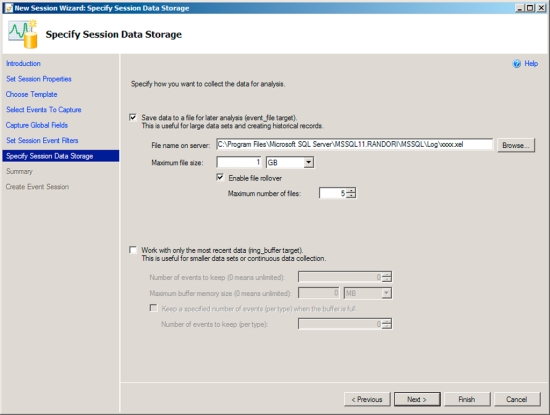
Figure 3-6. Specify Data Storage window in the New Session Wizard
As you can see it defaulted to local storage on my server. You can specify an appropriate location on your system. You can also decide if you’re using more than one file, how many, and whether or not those files rollover. All of those are management decisions that you’ll have to deal with as part of working with your environment and your sql query monitoring. You can run this 24/7, but you have to be prepared to deal with large amounts of data depending on how stringent the filters you’ve created are.
Finishing the Wizard and Starting the Session
Once you’ve defined the storage, you’ve set everything needed for the session. If you click the Next button, it will take you to a summary screen where you can review the settings you’ve chosen to ensure that the session reflects what you intended. Clicking finish will create the session in SQL Server. But, it won’t start the session. One of the beauties of Extended Events sessions is that they’re stored on the server and you can turn them on and off as needed. The Wizard finishes on a screen that gives you two options you can choose the start the session and, you can choose to start watching the data as it is captured to the screen.
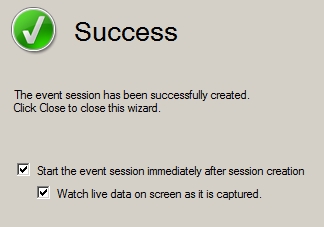
Figure 3-7. The Success screen of the Wizard
Watching the output from Extended Events doesn’t have the problems that the old Profiler GUI had where the GUI itself put an additional load on the system. These events are coming off the same buffer as the one that is writing out to disk, so you can watch events real time. Take a look at Figure 3-8 to see this in action:
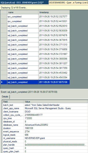
Figure 3-8. Live output of the extended event session created by the wizard
You can see the events on the top of the window showing the type of event and the date and time of the event. Clicking the event on the top will open the fields that were captured with the event on the bottom of the screen. As you can see, all the information we’ve been talking about is available to you. Also, if you’re unhappy with having a divided output, you can right-click a column and select “Show Column in Table” from the context menu. This will move it up into the top part of the screen, displaying all the information in a single location like Figure 3-9:
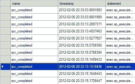
Figure 3-9. The statement column has been added to the table
Watching this information through the GUI and browsing through files is fine, but you’re going to want to automate the creation of these sessions. That’s what the next section covers.
The ability to use the GUI to build out a session and define the extended events you want to capture does make things very simple, but, unfortunately, it’s not a model that will scale. If you need to manage multiple servers where you’re going to create sessions for capturing key query performance metrics, you’re not going to want to connect to each one and go through the GUI to select the events, the output, etc. This is especially true if you take into account the chance of a mistake. Instead, it’s much better to learn how to work with sessions directly from TSQL. This will enable you to build a session that can be run on a number of servers in your system. Even better, you’re going to find that building sessions directly is easier in some ways than using the Wizard and you’re going to be much more knowledgeable about how these processes work.
Creating a Session Script Using the GUI
You can create a scripted trace in one of two ways, manually or with the GUI. Until you get comfortable with all the requirements of the scripts, the easy way is to use the Extended Events tool GUI. These are the steps you’ll need to perform:
1. Define a session (this time, outside the wizard).
2. Right-click the session, and select Script Sessions As, CREATE To, and File to output straight to a file.
These steps will generate all the script that you need to create a session and output it to a file.
To manually create this new trace, use Management Studio as follows:
1. Open the file.
2. Modify the path and file location for the server you’re creating this session on
3. Execute the script.
Once the sessions is created, you can use the following command to start it:
ALTER EVENT SESSION test_session
ON SERVER
STATE = start
You may want to automate the execution of the last step through the SQL Agent, or you can even run the script from the command line using the sqlcmd.exe utility. Whatever method you use, the final step will start the session. To stop the session, just run the same script with the STATE set to stop. I’ll show how to do that in the next section.
Defining a Session Using Stored Procedures
If you look at the script defined in the previous section, you will see a single command that was used to define the session, CREATE EVENT SESSION.
Once the session has been defined, you can activate it using ALTER EVENT.
Once a session is started on the server, you don’t have to keep Management Studio open any more. You can identify the active sessions by using the dynamic management view sys.dm_xe_sessions, as shown in the following query:
SELECT dxs.name,
dxs.create_time
FROM sys.dm_xe_sessions AS dxs;
Figure 3-10 shows the output of the view.
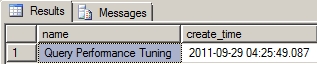
Figure 3-10. Output ofsys.dm_xe_sessions
The number of rows returned indicates the number of sessions active on SQL Server. You can stop a specific session by executing the stored procedure ALTER EVENT SESSION:
ALTER EVENT SESSION test_session
ON SERVER
STATE = stop;
To verify that the session is stopped successfully, reexecute the view sys.dm_xe_sessions, and ensure that the output of the view doesn’t contain the named session.
Using a script to create your sessions allows you to automate across a large number of servers. Using the scripts to start and stop the sessions means you can control them through scheduled events such as through SQL Agent. In Chapter 16, you will learn how to control the schedule of a session while capturing the activities of a SQL workload over an extended period of time.
![]() -1hd">Note The time captured through a session defined as illustrated in this section is stored in microseconds, not milliseconds. This difference between units can cause confusion if not taken into account. You must filter based on microseconds.
-1hd">Note The time captured through a session defined as illustrated in this section is stored in microseconds, not milliseconds. This difference between units can cause confusion if not taken into account. You must filter based on microseconds.
Extended Events Recommendations
Extended events are such a game-changer in the way that information is collected that many of the problematic areas that used to come up when using Trace Events have been completely eliminated. You just no longer need to worry as much about limiting the number of events collected or the number of fields returned. There are still a few areas you need to watch out for:
- Set max file size appropriately
- Avoid debug events
- Partition memory in the sessions
- Avoid use of No_Event_Loss
I’ll go over these in a little more detail in the following sections.
Set Max File Size Appropriately
If you use the Wizard to create a session, the default value for the files is 1gb. That’s actually very small when you consider the amount of information that can be gathered with extended events. It’s a good idea to set this number much higher, somewhere in the 50gb–100gb range to ensure you have adequate space to capture information and you’re not waiting on the file sub-system to create files for you while your buffer fills. This can lead to event loss. But, it does depend on your system. If you have a good grasp of the level of output you can expect, set the file size more appropriate to your individual environment.
Avoid Debug Events
Not only do extended events provide you with a mechanism for observing the behavior of SQL Server and it’s internals in a way that far exceeds what was possible under trace events, but Microsoft uses the same functionality as part of troubleshooting SQL Server. There are a number of events related to debugging SQL Server. These are not available through the Wizard, but you do have access to them through the TSQL command.
Do not use them. They are subject to change and are meant for Microsoft internal use only. If you do feel the need to experiment, you need to pay close attention to any of the events that include a break action. This means that should the event fire, it will stop SQL Server at the exact line of code that caused the event to fire. This means your server will be completely offline and in an unknown state. This could lead to a major outage if you were to do it in a production system. It could lead to loss of data and database corruption.
Partition Memory in the Sessions
For a simple set of events, such as those outlined earlier in the section on using the wizard, you don’t need to worry too much about partitioning your memory, but as the number of events you are collecting grows, you’re going to want to use the functions that will change the way that memory is handled in your sessions.
First, the default max for the buffer memory is 4mb. If you’re operating on a larger system and you are collecting a larger number of different events, you will want to raise this value. Specific numbers are hard to come by, so the guidance at this point must be vague. Changing the setting would be done by adding the command (for example, to double the buffer) to the TSQL code that creates the session:
MAX_MEMORY = 8192
Next, you can create multiple buffers on systems with multiple CPUs or on systems with Non-Uniform Memory Access (NUMA). To enable it on a system with multiple CPUs you would add the command:
MEMORY_PARTITION_MODE = Per_CPU
For a system with NUMA nodes configured you can use the following:
MEMORY_PARTITION_MODE = Per_Node
Either of these will break up the buffer and can provide you with improved performance in your extended event collection for some scenarios. You will need to test this for your environment.
Avoid Use of No_Event_Loss
Extended events are set up such that some events will be lost. It’s extremely likely, by design. But, you can use a setting, No_Event_Loss, when configuring your session. If you do this on systems that are already under load, you may see a significant additional load placed on the system since you’re effectively telling it to retain information in the buffer regardless of consequences. For very small and focused sessions that are targeting a particular behavior, this approach can be acceptable.
Other Methods for Query Performance Metrics
Setting up a session allows you to collect a lot of data for later use, but the collection can be a little bit expensive, you have to wait on the results, and then you have a lot of data to deal with. If you need to immediately capture performance metrics about your system, especially as they pertain to query performance, then the dynamic management views sys.dm_exec_query_stats for queries and sys.dm_exec_procedure_stats for stored procedures are what you need. If you still need a historical tracking of when queries were run and their individual costs, an extended events session is still the better tool. But if you just need to know, at this moment, the longest-running queries or the most physical reads, then you can get that information from these two dynamic management objects. The sys.dm_exec_query_stats DMO will return results for all queries, including stored procedures, but the sys.dm_exec_procedure_stats will only return information for stored procedures.
Since both these DMOs are just views, you can simply query against them and get information about the statistics of queries in the plan cache on the server. Table 3-5 shows some of the data returned from the sys.dm_exec_query_stats DMO.
Table 3-5. sys.dm_exec_query_stats Output
| Column | Description |
| Plan_handle | Pointer that refers to the execution plan |
| Creation_time | Time that the plan was created |
| Last_execution time | Last time the plan was used by a query |
| Execution_count | Number of times the plan has been used |
| Total_worker_time | Total CPU time used by the plan since it was created |
| Total_logical_reads | Total number of reads used since the plan was created |
| Total_logical_writes | Total number of writes used since the plan was created |
| Query_hash | A binary hash that can be used to identify queries with similar logic |
| Query_plan_hash | A binary hash that can be used to identify plans with similar logic |
Table 3-5 is just a sampling. For complete details, see Books Online.
To filter the information returned from sys.dm)exec_query_stats, you’ll need to join it with other dynamic management functions such as sys.dm_exec_sql_text, which shows the query text associated with the plan, or sys.dm_query_plan, which has the execution plan for the query. Once joined to these other DMOs, you can limit the database or procedure that you want to filter. These other DMOs are covered in detail in other chapters of the book. We’ll have examples of using sys.dm_exec_query_stats and the others, in combination, in this chapter, and throughout the rest of the book.
Now that you have seen two different ways of collecting query performance metrics, let’s look at what the data represents: the costly queries themselves. When the performance of SQL Server goes bad, two things are most likely happening:
- First, certain queries create high stress on system resources. These queries affect the performance of the overall system, because the server becomes incapable of serving other SQL queries fast enough.
- Additionally, the costly queries block all other queries requesting the same database resources, further degrading the performance of those queries. Optimizing the costly queries improves not only their own performance but also the performance of other queries by reducing database blocking and pressure on SQL Server resources.
- Finally, a query that, by itself is not terribly costly, could be called thousands of times a minute, which, by the simple accumulation of less than optimal code, can lead to major resource bottlenecks.
To begin to determine which queries you need to spend time working with, you’re going to use the resources that we’ve talked about so far. For example, assuming the queries are in cache, you will be able to use the DMOs to pull together meaningful data to determine the most costly queries. Alternatively, because you’ve captured the queries using extended events, you can access that data as a means to identify the costliest queries.
One small note on the extended events data: It’s going to be collected to a file. You’ll then need to load the data into a table or just query it directly. You can read directly from the extended events file you can query it using this system function:
SELECT *
FROM sys.fn_xe_file_target_read_file
('C:Program FilesMicrosoft SQL ServerMSSQL11.RANDORIMSSQLLogQuery Performance
Tuning*.xel’, NULL, NULL, NULL);
The query returns each extended event as a single row. The data about the event is stored in an XML column, event_data. You’ll need to use XQuery to go against the data directly, but once you do, you can search, sort and aggregate the data captured. I’ll walk you through a full example of this mechanism in the next section.
Identifying Costly Queries
The goal of SQL Server is to return result sets to the user in the shortest time. To do this, SQL Server has a built-in, cost-based optimizer called the query optimizer, which generates a cost-effective strategy called a query execution plan. The query optimizer weighs many factors, including (but not limited to) the usage of CPU, memory, and disk I/O required to execute a query, all derived from the statistics maintained by indexes or generated on the fly, and it then creates a cost-effective execution plan. Although minimizing the number of I/Os is not a requirement for a cost-effective plan, you will often find that the least costly plan generally has the fewest I/Os because I/O operations are expensive.
In the data returned from a session, the cpu_time and logical_reads or physical_reads fields also show where a query costs you. The cpu_time field represents the CPU time used to execute the query. The two reads fields represent the number of pages (8KB in size) a query operated on and thereby indicates the amount of memory or I/O stress caused by the query. It also provides an indication of disk stress, since memory pages have to be backed up in the case of action queries, populated during first-time data access, and displaced to disk during memory bottlenecks. The higher the number of logical reads for a query, the higher the possible stress on the disk could be. An excessive number of logical pages also increases load on the CPU in managing those pages. This is not an automatic correlation. You can’t always count on the query with the highest number of reads being the poorest performer. But it is a general metric and a good starting point.
The queries that cause a large number of logical reads usually acquire locks on a correspondingly large set of data. Even reading (as opposed to writing) may require shared locks on all the data, depending on the isolation level. These queries block all other queries requesting this data (or a part of the data) for the purposes of modifying it, not for reading it. Since these queries are inherently costly and require a long time to execute, they block other queries for an extended period of time. The blocked queries then cause blocks on further queries, introducing a chain of blocking in the database. (Chapter 12 covers lock modes.)
As a result, it makes sense to identify the costly queries and optimize them first, thereby doing the following:
- Improving the performance of the costly queries themselves
- Thereby reducing the overall stress on system resources
- Which can reduce database blocking
- Thereby reducing the overall stress on system resources
The costly queries can be categorized into the following two types:
- Single execution: An individual execution of the query is costly.
- Multiple executions: A query itself may not be costly, but the repeated execution of the query causes pressure on the system resources.
You can identify these two types of costly queries using different approaches, as explained in the following sections.
Costly Queries with a Single Execution
You can identify the costly queries by analyzing a session output file or by querying sys.dm_exec_query_stats. For this example, we’ll start with identifying queries that perform a large number of logical reads, so you should sort the trace output on the logical_reads data column. You can change that around to sort on duration, CPU, or even combine them in interesting ways. You can access the trace information by following these steps:
1. Capture a session that contains a typical workload.
2. Save the session output to a file.
3. Query the trace file for analysis Sorting by the logical_reads field
WITH xEvents AS
(SELECT object_name AS xEventName,
CAST (event_data AS xml) AS xEventData
FROM sys.fn_xe_file_target_read_file
('D:SessionsQueryPerformanceTuning*.xel', NULL, NULL, NULL)
)
SELECT
xEventName,
xEventData.value('(/event/data[@name=''duration'']/value)[1]','bigint') Duration,
xEventData.value('(/event/data[@name=''physical_reads'']/value)[1]','bigint') PhysicalReads,
xEventData.value('(/event/data[@name=''logical_reads'']/value)[1]','bigint') LogicalReads,
xEventData.value('(/event/data[@name=''cpu_time'']/value)[1]','bigint') CpuTime,
CASE xEventName WHEN 'sql_batch_completed' THEN
xEventData.value('(/event/data[@name=''batch_text'']/value)[1]','varchar(max)')
WHEN 'rpc_completed' THEN
xEventData.value('(/event/data[@name=''statement'']/value)[1]','varchar(max)')
END AS SQLText,
xEventData.value('(/event/data[@name=''query_plan_hash'']/value)[1]','binary(8)') QueryPlanHash
INTO Session_Table
FROM xEvents;
In some cases, you may have identified a large stress on the CPU from the System Monitor output. The pressure on the CPU may be because of a large number of CPU-intensive operations, such as stored procedure recompilations, aggregate functions, data sorting, hash joins, and so on. In such cases, you should sort the session output on the cpu_time field to identify the queries taking up a large number of processor cycles.
Costly Queries with Multiple Executions
As I mentioned earlier, sometimes a query may not be costly by itself, but the cumulative effect of multiple executions of the same query might put pressure on the system resources. In this situation, sorting on the logical_reads field won’t help you identify this type of costly query. You instead want to know the total number of reads, or total CPU time, or just the accumulated duration performed by multiple executions of the query.
- Query the session output and group on some of the values you’re interested in.
- Access the sys.dm_exec_query_stats DMO to retrieve the information from the production server. This assumes that you’re dealing with an immediate issue and not looking at a historical problem because this data is only what is currently in the procedure cache
Depending on the amount of data collected and the size of your files, running queries directly against the files you’ve collected from extended events may be excessively slow. In that case, use the same basic function, sys.fn_xe_file_target_read_file, to load the data into a table instead of querying it directly. Once that’s done, you can apply indexing to the table in order to speed up the queries. In this case, I’ll load the data into a table on the database so that I can run queries against it using the previous script.
Once the session data is imported into a database table, execute a SELECT statement to find the total number of reads performed by the multiple executions of the same query as follows (reads.sql in the download):
SELECT COUNT(*) AS TotalExecutions,
st.xEventName,
st.SQLText,
SUM(st.Duration) AS DurationTotal,
SUM(st.CpuTime) AS CpuTotal,
SUM(st.LogicalReads) AS LogicalReadTotal,
SUM(st.PhysicalReads) AS PhysicalReadTotal
FROM Session_Table AS st
GROUP BY st.xEventName, st.SQLText
ORDER BY LogicalReadTotal DESC;
The TotalExecutions column in the preceding script indicates the number of times a query was executed. The LogicalReadTotal column indicates the total number of logical reads performed by the multiple executions of the query.
The costly queries identified by this approach are a better indication of load than the costly queries with single execution identified by a session. For example, a query that requires 50 reads might be executed 1,000 times. The query itself may be considered cheap enough, but the total number of reads performed by the query turns out to be 50,000 (= 50 × 1,000), which cannot be considered cheap. Optimizing this query to reduce the reads by even 10 for individual execution reduces the total number of reads by 10,000 (= 10 × 1,000), which can be more beneficial than optimizing a single query with 5,000 reads.
The problem with this approach is that most queries will have a varying set of criteria in the WHERE clause or that procedure calls will have different values passed in. That makes the simple grouping by SqlText impossible. You can take care of this problem with a number of approaches. One of the better ones is outlined on the Microsoft Developers Network at http://msdn.microsoft.com/en-us/library/aal75800(SOL.8o).aspx. Although it was written originally for SQL Server 2000, it will work fine with SQL Server 2008.
Getting the same information out of the sys.dm_exec_query_stats view simply requires a query against the DMV:
SELECT s.totalexecutioncount,
t.text,
s.TotalExecutionCount,
s.TotalElapsedTime,
s.TotalLogicalReads,
s.TotalPhysicalReads
FROM (SELECT deqs.plan_handle,
SUM(deqs.execution_count) AS TotalExecutionCount,
SUM(deqs.total_elapsed_time) AS TotalElapsedTime,
SUM(deqs.total_logical_reads) AS TotalLogicalReads,
SUM(deqs.total_physical_reads) AS TotalPhysicalReads
FROM sys.dm_exec_query_stats AS deqs
GROUP BY deqs.plan_handle
) AS s
CROSS APPLY sys.dm_exec_sql_text(s.plan_handle) AS t
ORDER BY s.TotalLogicalReads DESC ;
Another mechanism you can apply to the data available from the execution DMOs is to use the query_hash and query_plan_hash as aggregation mechanisms. While a given stored procedure or parameterized query might have different values passed to it, changing the query_hash, the query_plan _hash for these will be identical. This means, you can aggregate against the hash values to identify common plans or common query patterns that you wouldn’t be able to see otherwise. This is just a slight modification from the previous query:
SELECT s.TotalExecutionCount,
t.text,
s.TotalExecutionCount,
s.TotalElapsedTime,
s.TotalLogicalReads,
s.TotalPhysicalReads
FROM (SELECT deqs.query_plan_hash,
SUM(deqs.execution_count) AS TotalExecutionCount,
SUM(deqs.total_elapsed_time) AS TotalElapsedTime,
SUM(deqs.total_logical_reads) AS TotalLogicalReads,
SUM(deqs.total_physical_reads) AS TotalPhysicalReads
FROM sys.dm_exec_query_stats AS deqs
GROUP BY deqs.query_plan_hash
AS s
CROSS APPLY (SELECT plan_handle
FROM sys.dm_exec_query_stats as deqs
WHERE s.query_plan_hash = deqs.query_plan_hash) AS p
CROSS APPLY sys.dm_exec_sql_text(p.plan_handle) AS t
ORDER BY TotalLogicalReads DESC ;
This is so much easier than all the work required to gather session data that it makes you wonder why you would ever use extended events at all. The main reason is precision. The sys.dm_exec_ query_stats view is a running aggregate for the time that a given plan has been in memory. Ann extended events session, on the other hand, is a historical track for whatever time frame you ran it in. You can even add session results together within a database and have a list of data that you can generate totals in a more precise manner rather than simply relying on a given moment in time. But understand that a lot of troubleshooting of performance problems is focused on that moment in time when the query is running slowly. That’s when sys.dm_exec_query_stats becomes irreplaceably useful.
Identifying Slow-Running Queries
Because a user’s experience is highly influenced by the response time of their requests, you should regularly monitor the execution time of incoming SQL queries and find out the response time of slow-running queries. If the response time (or duration) of slow-running queries becomes unacceptable, then you should analyze the cause of performance degradation. Not every slow-performing query is caused by resource issues, though. Other concerns such as blocking can also lead to slow query performance. Blocking is covered in detail in Chapter 12.
To identify slow running queries, just change the queries against your session data to change what you’re ordering by like this:
WITH xEvents AS
(SELECT object_name AS xEventName,
CAST (event_data AS xml) AS xEventData
FROM sys.fn_xe_file_target_read_file
('D:SessionQuery Performance Tuning*.xel', NULL, NULL, NULL)
)
SELECT
xEventName,
xEventData.value('(/event/data[@name=''duration'']/value)[1]','bigint') Duration,
xEventData.value('(/event/data[@name=''physical_reads'']/value)[1]','bigint') PhysicalReads,
xEventData.value('(/event/data[@name=''logical_reads'']/value)[1]','bigint') LogicalReads,
xEventData.value('(/event/data[@name=''cpu_time'']/value)[1]','bigint') CpuTime,
xEventData.value('(/event/data[@name=''batch_text'']/value)[1]','varchar(max)') BatchText,
xEventData.value('(/event/data[@name=''statement'']/value)[1]','varchar(max)') StatementText,
xEventData.value('(/event/data[@name=''query_plan_hash'']/value)[1]','binary(8)') QueryPlanHash
FROM xEvents
ORDER BY Duration DESC;
For a slow-running system, you should note the duration of slow-running queries before and after
the optimization process. After you apply optimization techniques, you should then work out the overall
effect on the system. It is possible that your optimization steps may have adversely affected other queries, making them slower.
Execution Plans
Once you have identified a costly query, you need to find out why it is so costly. You can identify the costly procedure from SQL Profiler or sys.dm_exec_procedure_stats, rerun it in Management Studio, and look at the execution plan used by the query optimizer. An execution plan shows the processing strategy (including multiple intermediate steps) used by the query optimizer to execute a query.
To create an execution plan, the query optimizer evaluates various permutations of indexes and join strategies. Because of the possibility of a large number of potential plans, this optimization process may take a long time to generate the most cost-effective execution plan. To prevent the overoptimization of an execution plan, the optimization process is broken into multiple phases. Each phase is a set of transformation rules that evaluate various permutations of indexes and join strategies ultimately attempting to find a good enough plan, not a perfect plan. It’s that difference between good enough and perfect that can lead to poor performance because of inadequately optimized execution plans. The query optimizer will only attempt a limited number of optimizations before it simply goes with the least costly plan it has currently.
After going through a phase, the query optimizer examines the estimated cost of the resulting plan. If the query optimizer determines that the plan is cheap enough, it will use the plan without going through the remaining optimization phases. However, if the plan is not cheap enough, the optimizer will go through the next optimization phase. I will cover execution plan generation in more depth in Chapter 9.
SQL Server displays a query execution plan in various forms and from two different types. The most commonly used forms in SQL Server 2012 are the graphical execution plan and the XML execution plan. Actually, the graphical execution plan is simply an XML execution plan parsed for the screen. The two types of execution plan are the estimated plan and the actual plan. The estimated plan represents the results coming from the query optimizer, and the actual plan is the plan used by the query engine. The beauty of the estimated plan is that it doesn’t require the query to be executed. The plans generated by these types can differ, but most of the time they will be the same. The primary difference is the inclusion of some execution statistics in the actual plan that are not present in the estimated plan.
The graphical execution plan uses icons to represent the processing strategy of a query. To obtain a graphical estimated execution plan, select Query Display Estimated Execution Plan. An XML execution plan contains the same data available through the graphical plan but in a more programmatically accessible format. Further, with the XQuery capabilities of SQL Server 2008, XML execution plans can be queried as if they were tables. An XML execution plan is produced by the statements SET SH0WPLAN_XML, for an estimated plan, and SET STATISTICS XML, for the actual execution plan. You can also right-click a graphical execution plan and select Showplan XML.
You can obtain the estimated XML execution plan for the costliest query identified previously using the SET SH0WPLAN_XML command as follows:
USE DATABASE AdventureWorks2008R2;
GO
SET SHOWPLAN_XML ON
GO
SELECT soh.AccountNumber,
sod.LineTotal,
sod.OrderQty,
sod.UnitPrice,
p.Name
FROM Sales.SalesOrderHeader soh
JOIN Sales.SalesOrderDetail sod
ON soh.SalesOrderID = sod.SalesOrderID
JOIN Production.Product p
ON sod.ProductID = p.ProductID
WHERE sod.LineTotal > 20000 ;
GO
SET SHOWPLAN_XML OFF
GO
Running this query results in a link to an execution plan, not an execution plan or any data. Clicking the link will open an execution plan. Although the plan will be displayed as a graphical plan, right-clicking the plan and selecting Show Execution Plan XML will display the XML data. Figure 3-11 shows a portion of the XML execution plan output.
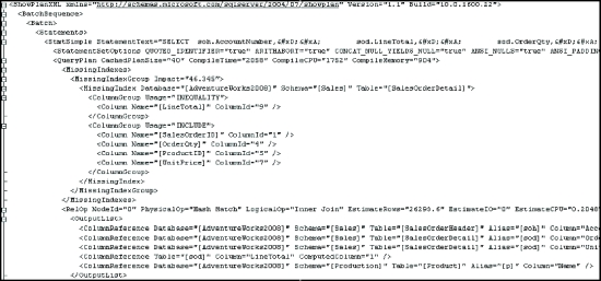
Figure 3-11. XML execution plan output
Analyzing a Query Execution Plan
Let’s start with the costly query identified in previous query. Copy it (minus the SET SHOWPLAN_XML statements) into Management Studio, and turn on Include Actual Execution Plan. Now, on executing this query, you’ll see the execution plan in Figure 3-12.
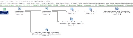
Execution plans show two different flows of information. Reading from the left side, you can see the logical flow, starting with the SELECT operator and proceeding through each of the execution steps. Starting from the right side and reading the other way is the physical flow of information, pulling data from the Index Scan operator first and then proceeding to each subsequent step.. Most of the time, reading in the direction of the physical flow of data is more applicable to understanding what’s happening with the execution plan. Each step represents an operation performed to get the final output of the query. Some of the aspects of a query execution represented by an execution plan are as follows:
- If a query consists of a batch of multiple queries, the execution plan for each query will be displayed in the order of execution. Each execution plan in the batch will have a relative estimated cost, with the total cost of the whole batch being 100 percent.
- Every icon in an execution plan represents an operator. They will each have a relative estimated cost, with the total cost of all the nodes in an execution plan being 100 percent.
- Usually the first physical operator in an execution represents a data-retrieval mechanism from a database object (a table or an index). For example, in the execution plan in Figure 3-10, the three starting points represent retrievals from the SalesOrderHeader, SalesOrderDetail, and Product tables.
- Data retrieval will usually be either a table operation or an index operation. For example, in the execution plan in Figure 3-10, all three data retrieval steps are index operations.
- Data retrieval on an index will be either an index scan or an index seek. For example, the first and second index operations in Figure 3-14 are index scans, and the third one is an index seek.
- The naming convention for a data-retrieval operation on an index is [Table Name]. [Index Name].
- Data flows from right to left between two operators and is indicated by a connecting arrow between the two operators.
- The thickness of a connecting arrow between operators represents a graphical representation of the number of rows transferred.
- The joining mechanism between two operators in the same column will be a nested loop join, a hash match join, or a merge join. For example, in the execution plan shown in Figure 3-14, there is one merge and one hash match. (Join mechanisms are covered in more detail later).
- Running the mouse over a node in an execution plan shows a pop-up window with some details, as you can see in Figure 3-13.
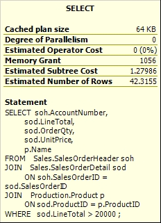
Figure 3-13. Tool-tip sheet from an execution plan operator
- A complete set of details about an operator is available in the Properties window, which you can open by right-clicking the operator and selecting Properties. This is visible in Figure 3-12.
- An operator detail shows both physical and logical operation types at the top. Physical operations represent those actually used by the storage engine, while the logical operations are the constructs used by the optimizer to build the estimated execution plan. If logical and physical operations are the same, then only the physical operation is shown. It also displays other useful information, such as row count, I/O cost, CPU cost, and so on.
- Reading through the properties on all operators can be necessary to understand how a query is being executed within SQL Server in order to better know how to tune that query.
Identifying the Costly Steps in an Execution Plan
The most immediate approach in the execution plan is to find out which steps are relatively costly. These steps are the starting point for your query optimization. You can choose the starting steps by adopting the following techniques:
- Each node in an execution plan shows its relative estimated cost in the complete execution plan, with the total cost of the whole plan being 100 percent. Therefore, focus attention on the node(s) with the highest relative cost. For example, the execution plan in Figure 3-10 has one step with 82 percent estimated cost.
- An execution plan may be from a batch of statements, so you may also need to find the most costly estimated statement. In Figure 3-15 and Figure 3-14, you can see at the top of the plan the text “Query 1.” In a batch situation, there will be multiple plans, and they will be numbered in the order they occurred within the batch.
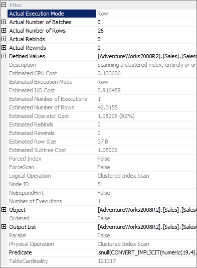
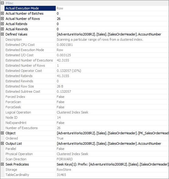
Figure 3-15. Data-retrieval mechanism for the SalesOrderHeader table
- Observe the thickness of the connecting arrows between nodes. A very thick connecting arrow indicates a large number of rows being transferred between the corresponding nodes. Analyze the node to the left of the arrow to understand why it requires so many rows. Check the properties of the arrows too. You may see that the estimated rows and the actual rows are different. This can be caused by out-of-date statistics, among other things.
- Look for hash join operations. For small result sets, a nested loop join is usually the preferred join technique. You will learn more about hash joins compared to nested loop joins later in this chapter. Just remember that hash joins are not necessarily bad, and loop joins are not necessarily good. It does depend on the amounts of data being returned by the query.
- Look for bookmark lookup operations. A bookmark operation for a large result set can cause a large number of logical reads. I will cover bookmark lookups in more detail in Chapter 6.
- There may be warnings, indicated by an exclamation point on one of the operators, which are areas of immediate concern. These can be caused by a variety of issues, including a join without join criteria or an index or a table with missing statistics. Usually resolving the warning situation will help performance.
- Look for steps performing a sort operation. This indicates that the data was not retrieved in the correct sort order.
- Watch for extra operators that may be placing additional load on the system such as table spools. These may be necessary for the operation of the query, or they may be indications of an improperly written query or badly designed indexes.
- The default cost threshold for parallel query execution is an estimated cost of 5 and that’s very low. Watch for parallel operations where they are not warranted.
To examine a costly step in an execution plan further, you should analyze the data-retrieval mechanism for the relevant table or index. First, you should check whether an index operation is a seek or a scan. Usually, for best performance, you should retrieve as few rows as possible from a table, and an index seek is usually the most efficient way of accessing a small number of rows. A scan operation usually indicates that a larger number of rows have been accessed. Therefore, it is generally preferable to seek rather than scan.
Next, you want to ensure that the indexing mechanism is properly set up. The query optimizer evaluates the available indexes to discover which index will retrieve data from the table in the most efficient way. If a desired index is not available, the optimizer uses the next best index. For best performance, you should always ensure that the best index is used in a data-retrieval operation. You can judge the index effectiveness (whether the best index is used or not) by analyzing the Argument section of a node detail for the following:
- A data-retrieval operation
- A join operation
Let’s look at the data-retrieval mechanism for the SalesOrderHeader table in the previous execution plan (Figure 3-12). Figure 3-15 shows the operator properties.
In the operator properties for the SalesOrderHeader table, the Object property specifies the index used, PK_SalesOrderHeader. It uses the following naming convention: [Database]. [Owner].[Table Name].
[Index Name]. The Seek Predicates property specifies the column, or columns, used to find keys in the index. The SalesOrderHeader table is joined with the SalesOrderDetail table on the SalesOrderld column. The SEEK works on the fact that the join criteria, SalesOrderld, is the leading edge of the clustered index and primary key, PK_SalesOrderHeader.
Sometimes you may have a different data-retrieval mechanism. Instead of the Seek Predicate that you
saw in Figure 3-15, Figure 3-16 shows a simple predicate, indicating a totally different mechanism for retrieving the data:.
In the properties in Figure 3-16, there is no seek predicate. Because of the function being performed on the column, the ISNULL and the CONVER_IMPLICIT, the entire table must be checked for existence of the Predicate value. Because a calculation is being performed on the data, the index doesn’t store the results of the calculation, so instead of simply looking information up on the index, you have to scan the data, performing the calculation, and then checking that the data is correct.
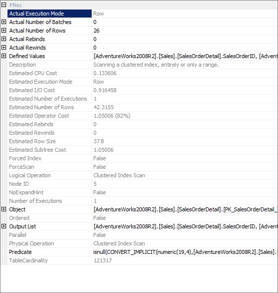
Figure 3-16. A variation of the data-retrieval mechanism, a scan
In addition to analyzing the indexes used, you should examine the effectiveness of join strategies decided by the optimizer. SQL Server uses three types of joins:
- Hash joins
- Merge joins
- Nested loop joins
In many simple queries affecting a small set of rows, nested loop joins are far superior to both hash and merge joins. The join types to be used in a query are decided dynamically by the optimizer.
To understand SQL Server’s hash join strategy, consider the following simple query:
SELECT p.*
FROM Production.Product p
JOIN Production.ProductCategory pc
ON p.ProductSubcategoryID = pc.ProductCategoryID;
Table 3-6 shows the two tables’ indexes and number of rows.
Table 3-6. Indexes and Number of Rows of the Products and ProductCategory Tables
| Table | indexes | Number of Rows |
| Product | Clustered index on ProductID | 504 |
| ProductCategory | Clustered index on ProductCategoryld | 4 |
Figure 3-17 shows the execution plan for the preceding query.
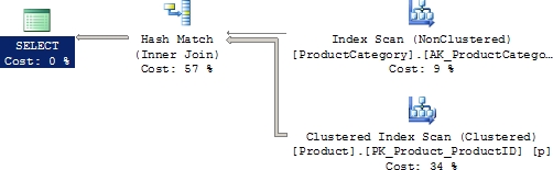
Figure 3-17. Execution plan with a hash join
You can see that the optimizer used a hash join between the two tables.
A hash join uses the two join inputs as a build input and a probe input. The build input is shown as the top input in the execution plan, and the probe input is shown as the bottom input. The smaller of the two inputs serves as the build input.
The hash join performs its operation in two phases: the build phase and the probe phase. In the most commonly used form of hash join, the in-memory hash join, the entire build input is scanned or computed, and then a hash table is built in memory. Each row is inserted into a hash bucket depending on the hash value computed for the hash key (the set of columns in the equality predicate).
This build phase is followed by the probe phase. The entire probe input is scanned or computed one row at a time, and for each probe row, a hash key value is computed. The corresponding hash bucket is scanned for the hash key value from the probe input, and the matches are produced. Figure 3-18 illustrates the process of an in-memory hash join.
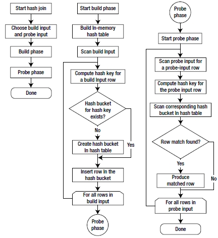
Figure 3-18. Workflow for an in-memory hash join
The query optimizer uses hash joins to process large, unsorted, nonindexed inputs efficiently. Let’s now look at the next type of join: the merge join.
In the previous case, input from the Product table is larger, and the table is not indexed on the joining column (ProductCategorylD). Using the following simple query, you can see different behavior:
SELECT pm.*
FROM Production.ProductModel pm
JOIN Production.ProductModelProductDescriptionCulture pmpd
ON pm.ProductModelID = pmpd.ProductModelID ;
Figure 3-19 shows the resultant execution plan for this query.
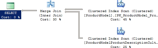
Figure 3-19. Execution plan with a merge join
For this query, the optimizer used a merge join between the two tables. A merge join requires both join inputs to be sorted on the merge columns, as defined by the join criterion. If indexes are available on both joining columns, then the join inputs are sorted by the index. Since each join input is sorted, the merge join gets a row from each input and compares them for equality. A matching row is produced if they are equal. This process is repeated until all rows are processed.
In situations where the data is ordered by an index, a merge join can be one of the fastest join operations, but if the data is no ordered and the optimizer still chooses to perform a merge join, then the data has to be ordered by an extra operation. This can make the merge join slower and more costly in terms of memory and I/O resources.
In this case, the query optimizer found that the join inputs were both sorted (or indexed) on their joining columns. As a result, the merge join was chosen as a faster join strategy than the hash join.
The final type of join I’ll cover here is the nested loop join. For better performance, you should always access a limited number of rows from individual tables. To understand the effect of using a smaller result set, decrease the join inputs in your query as follows:
SELECT soh.*
FROM Sales.SalesOrderHeader soh
JOIN Sales.SalesOrderDetail sod
ON soh.SalesOrderID = sod.SalesOrderID
WHERE soh.SalesOrderID = 71832 ;
Figure 3-20 shows the resultant execution plan of the new query.
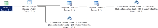
Figure 3-20. Execution plan with a nested loop join
As you can see, the optimizer used a nested loop join between the two tables.
A nested loop join uses one join input as the outer input table and the other as the inner input table. The outer input table is shown as the top input in the execution plan, and the inner input table is shown as the bottom input table. The outer loop consumes the outer input table row by row. The inner loop, executed for each outer row, searches for matching rows in the inner input table.
Nested loop joins are highly effective if the outer input is quite small and the inner input is large but indexed. In many simple queries affecting a small set of rows, nested loop joins are far superior to both hash and merge joins. Joins operate by gaining speed through other sacrifices. A loop join can be fast because it uses memory to take a small set of data and compare it quickly to a second set of data. A merge join similarly uses memory and a bit of tempdb to do its ordered comparisons. A hash join uses memory and tempdb to build out the hash tables for the join. Although a loop join is faster, it will consume more memory than a hash or merge as the data sets get larger, which is why SQL Server will use different plans in different situations for different sets of data.
Even for small join inputs, such as in the previous query, it’s important to have an index on the joining columns. As you saw in the preceding execution plan, for a small set of rows, indexes on joining columns allow the query optimizer to consider a nested loop join strategy. A missing index on the joining column of an input will force the query optimizer to use a hash join instead.
Table 3-7 summarizes the use of the three join types.
Table 3-7. Characteristics of the Three Join Types
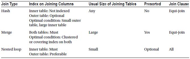
![]() Note The outer table is usually the smaller of the two joining tables in the hash and loop joins.
Note The outer table is usually the smaller of the two joining tables in the hash and loop joins.
I will cover index types, including clustered and covering indexes, in Chapter 4.
Actual vs. Estimated Execution Plans
There are estimated and actual execution plans. To a degree, these are interchangeable. But, the actual plan carries with it information from the execution of the query, specifically the row counts affected and some other information, that is not available in the estimated plans. This information can be extremely useful, especially when trying to understand statistic estimations. For that reason, actual execution plans are preferred when tuning queries.
Unfortunately, you won’t always be able to access them. You may not be able to execute a query, say in a production environment. You may only have access to the plan from cache, which contains no runtime information. So there are situations where the estimated plan is what you will have to work with.
However, there are other situations where the estimated plans will not work at all. Consider the following stored procedure (createpl.sql in the download):
IF (SELECT OBJECT_ID('p1')
) IS NOT NULL
DROP PROC p1
GO
CREATE PROC p1
AS
CREATE TABLE t1 (c1 INT) ;
INSERT INTO t1
SELECT ProductID
FROM Production.Product ;
SELECT *
FROM t1 ;
DROP TABLE t1 ;
GO
You may try to use SHOWPLANXML to obtain the estimated XML execution plan for the query as follows (showplan.sql in the download):
SET SHOWPLAN_XML ON
GO
EXEC p1 ;
GO
SET SHOWPLAN_XML OFF
GO
But this fails with the following error:
Msg 208, Level 16, State 1, Procedure p1, Line 3
Invalid object name 't1'..
Since SHOWPLANXML doesn’t actually execute the query, the query optimizer can’t generate an execution plan for INSERT and SELECT statements on the table (t1). Instead, you can use STATISTICS XML as follows:
SET STATISTICS XML ON
GO
EXEC p1;
GO
SET STATISTICS XML OFF
GO
Since STATISTICS XML executes the query, the table is created and accessed within the query which is all captured by the execution plan. Figure 3-21 shows the results of the query and the two plans for the two statements within the procedure provided by STATISTICS XML.
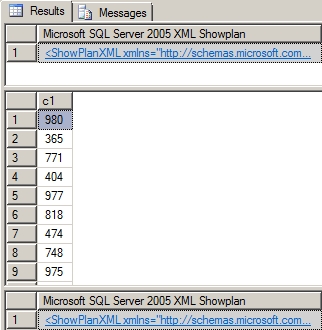
Figure 3-21. STATISTICS PROFILE output
![]() Tip Remember to switch Query Show Execution Plan off in Management Studio, or you will see the graphical, rather than textual, execution plan.
Tip Remember to switch Query Show Execution Plan off in Management Studio, or you will see the graphical, rather than textual, execution plan.
One final place to access execution plans is to read them directly from the memory space where they are stored, the plan cache. Dynamic management views and functions are provided from SQL Server to access this data. To see a listing of execution plans in cache, run the following query:
SELECT p.query_plan,
t.text
FROM sys.dm_exec_cached_plans r
CROSS APPLY sys.dm_exec_query_plan(r.plan_handle) p
CROSS APPLY sys.dm_exec_sql_text(r.plan_handle) t ;
The query returns a list of XML execution plan links. Opening any of them will show the execution plan. These execution plans are the compiled plans, but they contain no execution metrics. Working further with columns available through the dynamic management views will allow you to search for specific procedures or execution plans.
While not having the runtime data is somewhat limiting, having access to execution plans, even as the
query is executing, is an invaluable resource for someone working on performance tuning. As mentioned
earlier, you might not be able to execute a query in a production environment, so getting any plan at all is
useful.
Even though the execution plan for a query provides a detailed processing strategy and the estimated relative costs of the individual steps involved, it doesn’t provide the actual cost of the query in terms of CPU usage, reads/writes to disk, or query duration. While optimizing a query, you may add an index to reduce the relative cost of a step. This may adversely affect a dependent step in the execution plan, or sometimes it may even modify the execution plan itself. Thus, if you look only at the execution plan, you can’t be sure that your query optimization benefits the query as a whole, as opposed to that one step in the execution plan. You can analyze the overall cost of a query in different ways.
You should monitor the overall cost of a query while optimizing it. As explained previously, you can use Extended Events to monitor the duration, cpu, reads and writes information for the query. Extended events is an extremely efficient mechanism for gathering metrics. You should plan on taking advantage of this fact and use this mechanism to gather your query performance metrics. Just understand that collecting this information leads to large amounts of data that you will have to find a place to maintain within your system.
There are other ways to collect performance data that are more immediate than extended events.
Client statistics capture execution information from the perspective of your machine as a client of the server. This means that any times recorded include the time it takes to transfer data across the network, not merely the time involved on the SQL Server machine itself. To use them, simply click Query Include Client Statistics. Now, each time you run a query, a limited set of data is collected including execution time, the number of rows affected, round-trips to the server, and more. Further, each execution of the query is displayed separately on the Client Statistics tab, and a column aggregating the multiple executions shows the averages for the data collected. The statistics will also show whether a time or count has changed from one run to the next, showing up as arrows, as shown in Figure 3-22. For example, consider this query:
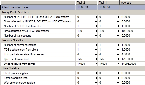
Figure 3-22. Client statistics
SELECT TOP 100 p.*
FROM Production.Product p
The client statistics information for the query should look something like that shown in Figure 3-22.
Although capturing client statistics can be a useful way to gather data, it’s a limited set of data, and there is no way to show how one execution is different from another. You could even run a completely different query, and its data would be mixed in with the others, making the averages useless. If you need to, you can reset the client statistics. Select the Query menu and then the Reset Client Statistics menu item.
Both Duration and CPU represent the time factor of a query. To obtain detailed information on the amount
of time (in milliseconds) required to parse, compile, and execute a query, use SET STATISTICS TIME
as follows:
SET STATISTICS TIME ON
GO
SELECT soh.AccountNumber,
sod.LineTotal,
sod.OrderQty,
sod.UnitPrice,
p.Name
FROM Sales.SalesOrderHeader soh
JOIN Sales.SalesOrderDetail sod
ON soh.SalesOrderID = sod.SalesOrderID
JOIN Production.Product p
ON sod.ProductID = p.ProductID
WHERE sod.LineTotal > 1000 ;
GO
SET STATISTICS TIME OFF
GO
The output of STATISTICS TIME for the preceding SELECT statement is as follows:
SQL Server parse and compile time:
CPU time = 0 ms, elapsed time = 0 ms.
(32101 row(s) affected)
SQL Server Execution Times:
CPU time = 516 ms, elapsed time = 1620 ms.
SQL Server parse and compile time:
CPU time = 0 ms, elapsed time = 2 ms.
The CPU time = 516 ms part of the execution times represents the CPU value provided by the Profiler tool and the Server Trace option. Similarly, the corresponding Elapsed time = 1620 ms represents the Duration value provided by the other mechanisms.
A 0 ms parse and compile time signifies that the optimizer reused the existing execution plan for this query and therefore didn’t have to spend any time parsing and compiling the query again. If the query is executed for the first time, then the optimizer has to parse the query first for syntax and then compile it to produce the execution plan. This can be easily verified by clearing out the cache using the system call DBCC FREEPROCCACHE and then rerunning the query:
SQL Server parse and compile time:
CPU time = 78 ms, elapsed time = 135 ms.
(32101 row(s) affected)
SQL Server Execution Times:
CPU time = 547 ms, elapsed time = 1318 ms.
SQL Server parse and compile time:
CPU time = 0 ms, elapsed time = 0 ms.
This time, SQL Server spent 78 ms of CPU time and a total of 135 ms parsing and compiling the query.
![]() Note You should not run DBCC FREEPROCCACHE on your production systems unless you are prepared to incur the not insignificant cost of recompiling every query on the system. In some ways, this will be as costly to your system as a reboot or a SQL Server instance restart.
Note You should not run DBCC FREEPROCCACHE on your production systems unless you are prepared to incur the not insignificant cost of recompiling every query on the system. In some ways, this will be as costly to your system as a reboot or a SQL Server instance restart.
As discussed in the “Identifying Costly Queries” section earlier in the chapter, the number of reads in the Reads column is frequently the most significant cost factor among duration, cpu, reads and writes. The total number of reads performed by a query consists of the sum of the number of reads performed on all tables involved in the query. The reads performed on the individual tables may vary significantly, depending on the size of the result set requested from the individual table and the indexes available.
To reduce the total number of reads, it will be useful to find all the tables accessed in the query and their corresponding number of reads. This detailed information helps you concentrate on optimizing data access on the tables with a large number of reads. The number of reads per table also helps you evaluate the impact of the optimization step (implemented for one table) on the other tables referred to in the query.
In a simple query, you determine the individual tables accessed by taking a close look at the query. This becomes increasingly difficult the more complex the query becomes. In the case of a stored procedure, database views, or functions, it becomes more difficult to identify all the tables actually accessed by the optimizer. You can use STATISTICS IO to get this information, irrespective of query complexity.
To turn STATISTICS IO on, navigate to Query Query Options Advanced Set Statistics IO in Management Studio. You may also get this information programmatically as follows:
SET STATISTICS IO ON
GO
SELECT soh.AccountNumber,
sod.LineTotal,
sod.OrderQty,
sod.UnitPrice,
p.Name
FROM Sales.SalesOrderHeader soh
JOIN Sales.SalesOrderDetail sod
ON soh.SalesOrderID = sod.SalesOrderID
JOIN Production.Product p
ON sod.ProductID = p.ProductID
WHERE sod.SalesOrderID = 71856 ;
GO
SET STATISTICS IO OFF
GO
If you run this query and look at the execution plan, it consists of three clustered index seeks with two loop joins. If you remove the WHERE clause and run the query again, you get a set of scans and some hash joins. That’s an interesting fact—but you don’t know how it affects the query cost! You can use SET STATISTICS IO as shown previously to compare the cost of the query (in terms of logical reads) between the two processing strategies used by the optimizer.
You get following STATISTICS IO output when the query uses the hash join:
Table 'Worktable'. Scan count 0, logical reads 0, physical reads 0…
Table 'SalesOrderDetail'. Scan count 1, logical reads 1240, physical reads 0…
Table 'SalesOrderHeader'. Scan count 1, logical reads 686, physical reads 0…
Table 'Product'. Scan count 1, logical reads 6, physical reads 0…
Now when you add back in the WHERE clause to appropriately filter the data, the resultant STATISTICS IO output turns out to be this:
Table 'Product'. Scan count 0, logical reads 4, physical reads 0…
Table 'SalesOrderDetail'. Scan count 1, logical reads 4, physical reads 0…
Table 'SalesOrderHeader'. Scan count 0, logical reads 3, physical reads 0…
Logical reads for the SalesOrderDetail table have been cut from 1,240 to 4 because of the index seek and the loop join. It also hasn’t significantly affected the data retrieval cost of the Product table.
While interpreting the output of STATISTICS IO, you mostly refer to the number of logical reads. Sometimes you also refer to the scan count, but even if you perform few logical reads per scan, the total number of logical reads provided by STATISTICS IO can still be high. If the number of logical reads per scan is small for a specific table, then you may not be able to improve the indexing mechanism of the table any further. The number of physical reads and read-ahead reads will be nonzero when the data is not found in the memory, but once the data is populated in memory, the physical reads and read-ahead reads will tend to be zero.
There is another advantage to knowing all the tables used and their corresponding reads for a query. Both the duration and CPU values may fluctuate significantly when reexecuting the same query with no change in table schema (including indexes) or data because the essential services and background applications running on the SQL Server machine usually affect the processing time of the query under observation. But, don’t forget that logical reads are not always the most accurate measure. Duration and CPU are absolutely useful and an important part of any query tuning.
During optimization steps, you need a nonfluctuating cost figure as a reference. The reads (or logical reads) don’t vary between multiple executions of a query with a fixed table schema and data. For example, if you execute the previous SELECT statement ten times, you will probably get ten different figures for duration and CPU, but Reads will remain the same each time. Therefore, during optimization, you can refer to the number of reads for an individual table to ensure that you really have reduced the data access cost of the table.
Even though the number of logical reads can also be obtained from the Extended Events, you get another benefit when using STATISTICS IO. The number of logical reads for a query shown by Profiler or the Server Trace option increases as you use different SET statements (mentioned previously) along with the query. But the number of logical reads shown by STATISTICS IO doesn’t include the additional pages that are accessed as SET statements are used with a query. Thus, STATISTICS IO provides a consistent figure for the number of logical reads.
Summary
In this chapter, you saw that you can use Extended Events to identify the queries causing a high amount of stress on the system resources in a SQL workload. Collecting the session data can, and should be, automated using system stored procedures. For immediate access to statistics about running queries, use the DMV sys.dm_exec_query_stats. You can further analyze these queries with Management Studio to find the costly steps in the processing strategy of the query. For better performance, it is important to consider both the index and join mechanisms used in an execution plan while analyzing a query. The number of data retrievals (or reads) for the individual tables provided by SET STATISTICS IO helps concentrate on the data access mechanism of the tables with most number of reads. You also should focus on the CPU cost and overall time of the most costly queries.
Once you identify a costly query and finish the initial analysis, the next step should be to optimize the query for performance. Because indexing is one of the most commonly used performance-tuning techniques, in the next chapter I will discuss in depth the various indexing mechanisms available in SQL Server.