
![]()
Windowing Functions
SQL Server is designed to work best on sets of data. By definition, sets of data are unordered; it is not until the query’s ORDER BY clause that the final results of the query become ordered. Windowing functions allow your query to look at a subset of the rows being returned by your query before applying the function to just those rows. In doing so, the functions allow you to specify an order for your unordered subset of data so as to evaluate that data in a particular order. This is performed before the final result is ordered (and in addition to it). This allows for processes that previously required self-joins, the use of inefficient inequality operators, or non-set-based row-by-row (iterative) processing to use more efficient set-based processing.
The key to windowing functions is in controlling the order in which the rows are evaluated, when the evaluation is restarted, and what set of rows within the result set should be considered for the function (the window of the data set that the function will be applied to). These actions are performed with the OVER clause.
There are three groups of functions that the OVER clause can be applied to; in other words, there are three groups of functions that can be windowed. These groups are the aggregate functions, the ranking functions, and the analytic functions. Additionally, the sequence object’s NEXT VALUE FOR function can be windowed. The functions that can have the OVER clause applied to them are shown in the following tables:
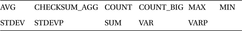
Table 7-1. Aggregate Functions
Ranking functions allow you to return a ranking value that is associated with each row in a partition of a result set. Depending on the function used, multiple rows may receive the same value within the partition, and there may be gaps between assigned numbers.
Table 7-2. Ranking Functions
|
Function |
Description |
|---|---|
|
ROW_NUMBER |
ROW_NUMBER returns an incrementing integer for each row within a partition of a set. ROW_NUMBER will return a unique number within each partition, starting with 1. |
|
RANK |
Similar to ROW_NUMBER, RANK increments its value for each row within a partition of the set. The key difference is that if rows with tied values exist within the partition, they will receive the same rank value, and the next value will receive the rank value as if there had been no ties, producing a gap between assigned numbers. |
|
DENSE_RANK |
The difference between DENSE_RANK and RANK is that DENSE_RANK doesn’t have gaps in the rank values when there are tied values; the next value has the next rank assignment. |
|
NTILE |
NTILE divides the result set into a specified number of groups, based on the ordering and optional partition clause. |
Analytic functions (introduced in SQL Server 2012) compute an aggregate value on a group of rows. In contrast to the aggregate functions, they can return multiple rows for each group.
Table 7-3. Analytic Functions
|
Function |
Description |
|---|---|
|
CUME_DIST |
CUME_DIST calculates the cumulative distribution of a value in a group of values. The cumulative distribution is the relative position of a specified value in a group of values. |
|
FIRST_VALUE |
Returns the first value from an ordered set of values. |
|
LAG |
Retrieves data from a previous row in the same result set as specified by a row offset from the current row. |
|
LAST_VALUE |
Returns the last value from an ordered set of values. |
|
LEAD |
Retrieves data from a subsequent row in the same result set as specified by a row offset from the current row. |
|
PERCENTILE_CONT |
Calculates a percentile based on a continuous distribution of the column value. The value returned may or may not be equal to any of the specific values in the column. |
|
PERCENTILE_DISC |
Computes a specific percentile for sorted values in the result set. The value returned will be the value with the smallest CUME_DIST value (for the same sort specification) that is greater than or equal to the specified percentile. The value returned will be equal to one of the values in the specific column. |
|
PERCENT_RANK |
Computes the relative rank of a row within a set. |
Many people will break down these functions into two groups: the LAG, LEAD, FIRST_VALUE, and LAST_VALUE functions are considered to be offset functions, and the remaining functions are called analytic functions. These functions come in complementary pairs, and many of the recipes will cover them in this manner.
The syntax for the OVER clause is as follows:
OVER (
 [ <PARTITION BY clause> ]
 [ <ORDER BY clause> ]
 [ <ROW or RANGE clause> ]
 )
The PARTITION BY clause is used to restart the calculations when the values in the specified columns change. It specifies columns from the tables in the FROM clause of the query, scalar functions, scalar subqueries, or variables. If a PARTITION BY clause isn’t specified, the entire data set will be the partition.
The ORDER BY clause defines the order in which the OVER clause evaluates the data subset for the function. It can only refer to columns that are in the FROM clause of the query.
The ROWS | RANGE clause defines a subset of rows that the window function will be applied to within the partition. If ROWS is specified, this subset is defined with the position of the current row relative to the other rows within the partition by position. If RANGE is specified, this subset is defined by the value(s) of the column(s) in the current row relative to the other rows within the partition. This range is defined as a beginning point and an ending point. For both ROWS and RANGE, the beginning point can be UNBOUNDED PRECEDING or CURRENT ROW, and the ending point can be UNBOUNDED FOLLOWING or CURRENT ROW, where UNBOUNDED PRECEDING means the first row in the partition, UNBOUNDED FOLLOWING means the last row in the partition, and CURRENT ROW is just that—the current row. Additionally, when ROWS is specified, an offset can be specified with <X> PRECEDING or <X> FOLLOWING, which is simply the number of rows prior to or following the current row. Additionally, there are two methods to specify the subset range—you can specify just the beginning point (which will use the default CURRENT ROW as the default ending point), or you can specify both with the BETWEEN <starting point> AND <ending point> syntax. Finally, the entire ROWS | RANGE clause itself is optional; if it is not specified, the default ROWS | RANGE clause will default to RANGE BETWEEN UNBOUNDED PRECEDING AND CURRENT ROW.
Each of the windowing functions permits and requires various clauses from the OVER clause.
With the exception of the CHECKSUM, GROUPING, and GROUPING_ID functions, all of the aggregate functions can be windowed through the use of the OVER clause, as shown in Table 7-1 above. Additionally, the ROWS | RANGE clause allows you to perform running aggregations and sliding (moving) aggregations.
The first four recipes in this section utilize the following table and data:
CREATE TABLE #Transactions
       (
        AccountId INTEGER,
        TranDate DATE,
        TranAmt NUMERIC(8, 2)
       );
INSERT  INTO #Transactions
SELECT  *
FROM    ( VALUES ( 1, '2011-01-01', 500),
                 ( 1, '2011-01-15', 50),
                 ( 1, '2011-01-22', 250),
                 ( 1, '2011-01-24', 75),
                 ( 1, '2011-01-26', 125),
                 ( 1, '2011-01-26', 175),
                 ( 2, '2011-01-01', 500),
                 ( 2, '2011-01-15', 50),
                 ( 2, '2011-01-22', 25),
                 ( 3, '2011-01-22', 5000),
                 ( 3, '2011-01-27', 550),
                 ( 3, '2011-01-27', 95 ),
                 ( 3, '2011-01-30', 2500)
        ) dt (AccountId, TranDate, TranAmt);
Note that within AccountIDs 1 and 3, there are two rows that have the same TranDate value. This duplicate date will be used to highlight the differences in some of the clauses used in the OVER clause in subsequent recipes.
7-1. Calculating Totals Based upon the Prior Row
Problem
You need to calculate the total of a column, where the total is the sum of the column values through the current row. For instance, for each account, calculate the total transaction amount to date in date order.
Solution
Utilize the SUM function with the OVER clause to perform a running total:
SELECT  AccountId,
        TranDate,
        TranAmt,
       -- running total of all transactions
        RunTotalAmt = SUM(TranAmt) OVER (PARTITION BY AccountId ORDER BY TranDate)
FROM    #Transactions AS t
ORDER BY AccountId,
        TranDate;
This query returns the following result set:
AccountId   TranDate   TranAmt RunTotalAmt
----------- ---------- ------- -----------
1           2011-01-01 500.00  500.00
1           2011-01-15 50.00   550.00
1           2011-01-22 250.00  800.00
1           2011-01-24 75.00   875.00
1           2011-01-26 125.00  1175.00
1           2011-01-26 175.00  1175.00
2           2011-01-01 500.00  500.00
2           2011-01-15 50.00   550.00
2           2011-01-22 25.00   575.00
3           2011-01-22 5000.00 5000.00
3           2011-01-27 550.00  5645.00
3           2011-01-27 95.00   5645.00
3           2011-01-30 2500.00 8145.00
How It Works
The OVER clause, when used in conjunction with the SUM function, allows us to perform a running total of the transaction. Within the OVER clause, the PARTITION BY clause is specified so as to restart the calculation every time the AccountId value changes. The ORDER BY clause is specified and determines in which order the rows should be calculated. Since the ROWS | RANGE clause is not specified, the default RANGE BETWEEN UNBOUNDED PRECEDING AND CURRENT ROW is utilized. When the query is executed, the TranAmt column from all of the rows prior to and including the current row is summed up and returned.
In this example, for the first row for each AccountID value, the RunTotalAmt returned is simply the value from the TotalAmt column from the row. For subsequent rows, this value is incremented by the value in the current row’s TotalAmt column. When the AccountID value changes, the running total is reset and recalculated for the new AccountID value. So, for AccountID = 1, the RunTotalAmt value for TranDate 2011-01-01 is 500 (the value of that row’s TranAmt column). For the next row (TranDate 2011-01-1), the TranAmt of 50 is added to the 500 for a running total of 550. In the next row (TranDate 2011-01-22), the TranAmt of 250 is added to the 550 for a running total of 800.
Note the duplicate TranDate value within each AccountID value—the running total did not increment in the way that you would expect it to. Since this query did not specify a ROWS | RANGE clause, the default of RANGE BETWEEN UNBOUNDED PRECEDING AND CURRENT ROW was utilized. RANGE does not work on a row-position basis; instead, it works off of the values in the columns. For the rows with the duplicate TranDate, the TranAmt for all of the rows with that duplicate value were summed together. To see the data in the manner in which you would most likely want to see a running total, modify the query to include an additional column that performs the same running total calculation with the ROWS clause:
SELECT  AccountId,
        TranDate,
        TranAmt,
        -- running total of all transactions
        RunTotalAmt =   SUM(TranAmt) OVER (PARTITION BY AccountId ORDER BY TranDate),
        -- "Proper" running total by row position
        RunTotalAmt2 =  SUM(TranAmt) OVER (PARTITION BY AccountId
                                           ORDER BY TranDate
                                           ROWS UNBOUNDED PRECEDING)
FROM    #Transactions AS t
ORDER BY AccountId,
        TranDate;
This query produces these more desirable results in the RunTotalAmt2 column:
AccountId   TranDate   TranAmt RunTotalAmt RunTotalAmt2
----------- ---------- ------- ----------- ------------
1           2011-01-01 500.00  500.00      500.00
1           2011-01-15 50.00   550.00      550.00
1           2011-01-22 250.00  800.00      800.00
1           2011-01-24 75.00   875.00      875.00
1           2011-01-26 125.00  1175.00     1000.00
1           2011-01-26 175.00  1175.00     1175.00
2           2011-01-01 500.00  500.00      500.00
2           2011-01-15 50.00   550.00      550.00
2           2011-01-22 25.00   575.00      575.00
3           2011-01-22 5000.00 5000.00     5000.00
3           2011-01-27 550.00  5645.00     5550.00
3           2011-01-27 95.00   5645.00     5645.00
3           2011-01-30 2500.00 8145.00     8145.00
Running aggregations can be performed over the other aggregate functions. In this next example, the query is modified to perform running averages, counts, and minimum/maximum calculations.
SELECT  AccountId,
        TranDate,
        TranAmt,
       -- running average of all transactions
        RunAvg = AVG(TranAmt) OVER (PARTITION BY AccountId ORDER BY TranDate),
       -- running total # of transactions
        RunTranQty = COUNT(*) OVER (PARTITION BY AccountId ORDER BY TranDate),
       -- smallest of the transactions so far
        RunSmallAmt = MIN(TranAmt) OVER (PARTITION BY AccountId ORDER BY TranDate),
       -- largest of the transactions so far
        RunLargeAmt = MAX(TranAmt) OVER (PARTITION BY AccountId ORDER BY TranDate),
       -- running total of all transactions
        RunTotalAmt = SUM(TranAmt) OVER (PARTITION BY AccountId ORDER BY TranDate)
FROM    #Transactions AS t
WHERE   AccountID = 1
ORDER BY AccountId, TranDate;
This query returns the following result set:
AccountId   TranDate   TranAmt RunAvg      RunTranQty  RunSmallAmt RunLargeAmt RunTotalAmt
----------- ---------- ------- ----------- ----------- ----------- ----------- -----------
1           2011-01-01 500.00  500.000000  1           500.00      500.00      500.00
1           2011-01-15 50.00   275.000000  2           50.00       500.00      550.00
1           2011-01-22 250.00  266.666666  3           50.00       500.00      800.00
1           2011-01-24 75.00   218.750000  4           50.00       500.00      875.00
1           2011-01-26 125.00  195.833333  6           50.00       500.00      1175.00
1           2011-01-26 175.00  195.833333  6           50.00       500.00      1175.00
7-2. Calculating Totals Based upon a Subset of Rows
Problem
When performing these aggregations, you want only the current row and the two previous rows to be considered for the aggregation.
Solution
Utilize the ROWS clause of the OVER clause:
SELECT AccountId,
       TranDate,
       TranAmt,
       -- average of the current and previous 2 transactions
       SlideAvg = AVG(TranAmt)
                  OVER (PARTITION BY AccountId
                            ORDER BY TranDate
                             ROWS BETWEEN 2 PRECEDING AND CURRENT ROW),
       -- total # of the current and previous 2 transactions
       SlideQty  = COUNT(*)
                    OVER (PARTITION BY AccountId
                              ORDER BY TranDate
                               ROWS BETWEEN 2 PRECEDING AND CURRENT ROW),
       -- smallest of the current and previous 2 transactions
       SlideMin = MIN(TranAmt)
                  OVER (PARTITION BY AccountId
                            ORDER BY TranDate
                             ROWS BETWEEN 2 PRECEDING AND CURRENT ROW),
       -- largest of the current and previous 2 transactions
       SlideMax = MAX(TranAmt)
                  OVER (PARTITION BY AccountId
                            ORDER BY TranDate
                             ROWS BETWEEN 2 PRECEDING AND CURRENT ROW),
       -- total of the current and previous 2 transactions
       SlideTotal = SUM(TranAmt)
                    OVER (PARTITION BY AccountId
                              ORDER BY TranDate
                               ROWS BETWEEN 2 PRECEDING AND CURRENT ROW)
FROM    #Transactions AS t
ORDER BY AccountId, TranDate;
This query returns the following result set:
AccountId   TranDate   TranAmt SlideAvg    SlideQty SlideMin SlideMax SlideTotal
----------- ---------- ------- ----------- -------- -------- -------- ----------
1           2011-01-01 500.00  500.000000  1        500.00   500.00   500.00
1           2011-01-15 50.00   275.000000  2        50.00    500.00   550.00
1           2011-01-22 250.00  266.666666  3        50.00    500.00   800.00
1           2011-01-24 75.00   125.000000  3        50.00    250.00   375.00
1           2011-01-26 125.00  150.000000  3        75.00    250.00   450.00
1           2011-01-26 175.00  125.000000  3        75.00    175.00   375.00
2           2011-01-01 500.00  500.000000  1        500.00   500.00   500.00
2           2011-01-15 50.00   275.000000  2        50.00    500.00   550.00
2           2011-01-22 25.00   191.666666  3        25.00    500.00   575.00
3           2011-01-22 5000.00 5000.000000 1        5000.00  5000.00  5000.00
3           2011-01-27 550.00  2775.000000 2        550.00   5000.00  5550.00
3           2011-01-27 95.00   1881.666666 3        95.00    5000.00  5645.00
3           2011-01-30 2500.00 1048.333333 3        95.00    2500.00  3145.00
How It Works
The ROWS clause is added to the OVER clause of the aggregate functions to specify that the aggregate functions should look only at the current row and the previous two rows for their calculations. As you look at each column in the result set, you can see that the aggregation was performed over just these rows (the window of rows that the aggregation is applied to). As the query progresses through the result set, the window slides to encompass the specified rows relative to the current row.
Let’s examine the results row by row for AccountID 1. Remember that we are applying a subset (ROWS clause) to be the current row and the two previous rows. For TranDate 2011-01-01, there are no previous rows. For the COUNT calculation, there is just one row, so SlideQty returns 1. For each of the other columns (SlideAvg, SlideMin, SlideMax, SlideTotal), there are no previous rows, so the current row’s TranAmt is returned as the AVG, MIN, MAX, and SUM values.
For the second row (TranDate 2011-01-15), there are now two rows “visible” in the subset of data, starting from the first row. The COUNT calculation sees these two and returns 2 for the SlideQty. The AVG calculation of these two rows is 275: (500 + 50) / 2. The MIN of these two values (500, 50) is 50. The MAX of these two values is 500. And finally, the SUM (total) of these two values is 550. These are the values returned in the SlideAvg, SlideMin, SlideMax, and SlideTotal columns.
For the third row (TranDate 2011-01-15), there are now three rows “visible” in the subset of data, starting from the first row. The COUNT calculation sees these three and returns 3 for the SlideQty. The AVG calculation of the TranAmt column for these three rows is 266.66: (500 + 50 + 250) / 3. The MIN of these three values (500, 50, 250) is still 50, and the MAX of these three values is still 500. And finally, the SUM (total) of these three values is 800. These are the values returned in the SlideAvg, SlideMin, SlideMax, and SlideTotal columns.
For the fourth row (TranDate 2011-01-24), we still have three rows “visible” in the subset of data; however, we have started our sliding / moving aggregation window—the window starts with the second row and goes through the current (fourth) row. The COUNT calculation still sees that we are applying the function to only three rows, so it returns 3 in the SlideQty column. The AVG calculation of the TranAmt column for the three rows is applied over the values (50, 250, 75), which produces an average of 125: (50 + 250 + 75) / 3. The MIN of the three values is still 50, while the MAX of these three values is now 250. The SUM total of these three values is 375. Again, these are the values returned in the SlideAvg, SlideMin, SlideMax, and SlideTotal columns.
As we progress to the fifth row (TranDate 2011-01-26 and TranAmt 125.00), the window slides again. We are still looking at only three rows (the third row through the fifth row), so SlideQty still returns 3. The other calculations are looking at the TranAmt values of 250, 75, 125 for these three rows, so the AVG, MIN, MAX, and SUM calculations are 150, 75, 250, and 450.
For the sixth row, the window again slides, and the calculations are recalculated for the new subset of data. For the seventh row, we now have the AccountID changing from 1 to 2. Since the query has a PARTITION BY clause set on the AccountID column, the calculations are reset. The seventh row of the result set is the first row for this partition (AccountID), so the SlideQty is 1, and the other columns will have for the AVG, MIN, MAX, and SUM calculations the value of the TranAmt column. The sliding window continues as defined above.
7-3. Calculating a Percentage of Total
Problem
With each row in your result set, you want to have the data included so that you are able to calculate what percentage of the total the row is.
Solution
Use the SUM function with the OVER clause without specifying any ordering so as to have each row return the total for that partition:
SELECT  AccountId,
        TranDate,
        TranAmt,
        AccountTotal = SUM(TranAmt) OVER (PARTITION BY AccountId),
        AmountPct = TranAmt / SUM(TranAmt) OVER (PARTITION BY t.AccountId)
FROM    #Transactions AS t
This query returns the following result set (AmountPct column truncated at 7 decimals for brevity):
AccountId   TranDate   TranAmt AccountTotal AmountPct
----------- ---------- ------- ------------ ---------
1           2011-01-01 500.00  1175.00      0.4255319
1           2011-01-15 50.00   1175.00      0.0425531
1           2011-01-22 250.00  1175.00      0.2127659
1           2011-01-24 75.00   1175.00      0.0638297
1           2011-01-26 125.00  1175.00      0.1063829
1           2011-01-26 175.00  1175.00      0.1489361
2           2011-01-01 500.00  575.00       0.8695652
2           2011-01-15 50.00   575.00       0.0869565
2           2011-01-22 25.00   575.00       0.0434782
3           2011-01-22 5000.00 8145.00      0.6138735
3           2011-01-27 550.00  8145.00      0.0675260
3           2011-01-27 95.00   8145.00      0.0116635
3           2011-01-30 2500.00 8145.00      0.3069367
How It Works
When the SUM function is utilized with the OVER clause, and the OVER clause does not contain the ORDER BY clause, then the SUM function will return the total amount for the partition. The current row’s value can be divided by this total to obtain the percentage of the total that the current row is. If the ORDER BY clause had been included, then a ROWS | RANGE clause would have been used; if one wasn’t specified, then the default RANGE BETWEEN UNBOUNDED PRECEDING AND CURRENT ROW would have been used, as shown in recipe 7-1.
If you wanted to get the total for the entire result set instead of the total for each partition (in this example, AccountId), you would use:
SELECT  AccountId,
        TranDate,
        TranAmt,
        Total = SUM(TranAmt) OVER (),
        AmountPct = TranAmt / SUM(TranAmt) OVER ()
FROM    #Transactions AS t
ORDER BY AccountId, TranDate;
7-4. Calculating a “Row X of Y”
Problem
You want your result set to display a “Row X of Y,” where X is the current row number and Y is the total number of rows.
Solution
Use the ROW_NUMBER function to obtain the current row number, and the COUNT function with the OVER clause to obtain the total number of rows:
SELECT  AccountId,
        TranDate,
        TranAmt,
        AcctRowID = ROW_NUMBER() OVER (PARTITION BY AccountId ORDER BY AccountId, TranDate),
        AcctRowQty = COUNT(*) OVER (PARTITION BY AccountId),
        RowID = ROW_NUMBER() OVER (ORDER BY AccountId, TranDate),
        RowQty = COUNT(*) OVER ()
FROM    #Transactions AS t
ORDER BY AccountId, TranDate;;
This query returns the following result set:
AccountId   TranDate   TranAmt AcctRowID AcctRowQty RowID RowQty
----------- ---------- ------- --------- ---------- ----- ------
1           2011-01-01 500.00  1         6          1     13
1           2011-01-15 50.00   2         6          2     13
1           2011-01-22 250.00  3         6          3     13
1           2011-01-24 75.00   4         6          4     13
1           2011-01-26 125.00  5         6          5     13
1           2011-01-26 175.00  6         6          6     13
2           2011-01-01 500.00  1         3          7     13
2           2011-01-15 50.00   2         3          8     13
2           2011-01-22 25.00   3         3          9     13
3           2011-01-22 5000.00 1         4          10    13
3           2011-01-27 550.00  2         4          11    13
3           2011-01-27 95.00   3         4          12    13
3           2011-01-30 2500.00 4         4          13    13
How It Works
The ROW_NUMBER function is used to get the current row number within a partition, and the COUNT function is used to get the total number of rows within a partition. Both the ROW_NUMBER and COUNT functions are used twice, once with a PARTITION BY clause and once without. The ROW_NUMBER function returns a sequential number (as ordered by the specified ORDER BY clause in the OVER clause) for each row that has the partition specified. In the AcctRowID column, this is partitioned by the AccountId, so the sequential numbering will restart upon each change in the AccountId column; in the RowID column, a PARTITION BY is not specified, so this will return a sequential number for each row with the entire result set. Likewise for the COUNT function: the AcctRowQty column is partitioned by the AccountID column, so this will return, for each row, the number of rows within this partition (AccountId). The RowQty column is not partitioned, so this will return the total number of rows in the entire result set. The corresponding columns (AcctRowID, AcctRowQty and RowID, RowQty) utilize the same PARTITION BY clause (or lack of) in order to make the results meaningful.
For each row for AccountID = 1, the AcctRowID column will return a sequential number for each row, and the AcctRowQty column will return 6 (since there are 6 rows for this account). In a similar way, the RowID column will return a sequential number for each row in the result set, and the RowQty will return the total number of rows in the result set (13), since both of these are calculated without a PARTITION BY clause. For the first row where AccountId = 1, this will be row 1 of 6 within AccountId 1, and row 1 of 13 within the entire result set. The second row will be 2 of 6 and 2 of 13, and this proceeds through the remaining rows for this AccountId. When we get to AccountId = 2, the AcctRowID and AcctRowQty columns reset (due to the PARTITION BY clause), and return row 1 of 3 for the AccountId, and row 7 of 13 for the entire result set.
7-5. Using a Logical Window
Problem
You want the rows being considered by the OVER clause to be affected by the value in the column instead of the row positioning as determined by the ORDER BY clause in the OVER clause.
Solution
In the OVER clause, utilize the RANGE clause instead of the ROWS option:
CREATE TABLE #Test
        (
         RowID INT IDENTITY,
         FName VARCHAR(20),
         Salary SMALLINT
        );

INSERT INTO #Test (FName, Salary)
VALUES ('George',       800),
       ('Sam',          950),
       ('Diane',       1100),
       ('Nicholas',    1250),
       ('Samuel',      1250),  --<< duplicate value of above row
       ('Patricia',    1300),
       ('Brian',       1500),
       ('Thomas',      1600),
       ('Fran',        2450),
       ('Debbie',      2850),
       ('Mark',        2975),
       ('James',       3000),
       ('Cynthia',     3000),  --<< duplicate value of above row
       ('Christopher', 5000);

SELECT RowID,
       FName,
       Salary,
       SumByRows  = SUM(Salary) OVER (ORDER BY Salary ROWS UNBOUNDED PRECEDING),
       SumByRange = SUM(Salary) OVER (ORDER BY Salary RANGE UNBOUNDED PRECEDING)
FROM   #Test
ORDER BY RowID;
This query returns the following result set:
RowID       FName                Salary SumByRows   SumByRange
----------- -------------------- ------ ----------- -----------
1           George               800    800         800
2           Sam                  950    1750        1750
3           Diane                1100   2850        2850
4           Nicholas             1250   4100        5350
5           Samuel               1250   5350        5350
6           Patricia             1300   6650        6650
7           Brian                1500   8150        8150
8           Thomas               1600   9750        9750
9           Fran                 2450   12200       12200
10          Debbie               2850   15050       15050
11          Mark                 2975   18025       18025
12          James                3000   21025       24025
13          Cynthia              3000   24025       24025
14          Christopher          5000   29025       29025
How It Works
When utilizing the RANGE clause, the SUM function adjusts its window based upon the values in the specified column. The window is sized upon the beginning- and ending-point boundaries specified; in this case, the beginning point of UNBOUNDED PRECEDING (the first row in the partition) was specified, and the default ending boundary of CURRENT ROW was used. This example shows the salary of your employees, and the SUM function is performing a running total of the salaries in order of the salary. For comparison purposes, the running total is being calculated with both the ROWS and RANGE clauses. Within this dataset, there are two groups of employees that have the same salary: RowIDs 4 and 5 are both 1,250, and 12 and 13 are both 3,000. When the running total is calculated with the ROWS clause, you can see that the salary of the current row is being added to the prior total of the previous rows. However, when the RANGE clause is used, all of the rows that contain the value of the current row are totaled and added to the total of the previous value. The result is that for rows 4 and 5, both employees with a salary of 1,250 are added together for the running total (and this action is repeated for rows 12 and 13).
![]() Tip If you need to perform running aggregations, and there is the possibility that you can have multiple rows with the same value in the columns specified by the ORDER BY clause, you should use the ROWS clause instead of the RANGE clause.
Tip If you need to perform running aggregations, and there is the possibility that you can have multiple rows with the same value in the columns specified by the ORDER BY clause, you should use the ROWS clause instead of the RANGE clause.
7-6. Generating an Incrementing Row Number
Problem
You need to have a query return total sales information. You need to include a row number for each row that corresponds to the order of the date of the purchase (so as to show the sequence of the transactions), and the numbering needs to start over for each account number.
Solution
Utilize the ROW_NUMBER function to assign row numbers to each row:
SELECT TOP 10
        AccountNumber,
        OrderDate,
        TotalDue,
        ROW_NUMBER() OVER (PARTITION BY AccountNumber ORDER BY OrderDate) AS RowNumber
FROM    AdventureWorks2014.Sales.SalesOrderHeader
ORDER BY AccountNumber;
This query returns the following result set:
AccountNumber   OrderDate               TotalDue              RN
--------------- ----------------------- --------------------- --
10-4020-000001  2005-08-01 00:00:00.000 12381.0798            1
10-4020-000001  2005-11-01 00:00:00.000 22152.2446            2
10-4020-000001  2006-02-01 00:00:00.000 31972.1684            3
10-4020-000001  2006-05-01 00:00:00.000 29418.5269            4
10-4020-000002  2006-08-01 00:00:00.000 8727.1055             1
10-4020-000002  2006-11-01 00:00:00.000 4682.6908             2
10-4020-000002  2007-02-01 00:00:00.000 1485.918              3
10-4020-000002  2007-05-01 00:00:00.000 1668.3751             4
10-4020-000002  2007-08-01 00:00:00.000 3478.1096             5
10-4020-000002  2007-11-01 00:00:00.000 3941.9843             6
How It Works
The ROW_NUMBER function is utilized to generate a row number for each row in the partition. The PARTITION_BY clause is utilized to restart the number generation for each change in the AccountNumber column. The ORDER_BY clause is utilized to order the numbering of the rows by the value in the OrderDate column.
You can also utilize the ROW_NUMBER function to create a virtual numbers, or tally, table. (A numbers, or tally, table is simply a table of sequential numbers, and it can be utilized to eliminate loops. Use your favorite Internet search tool to find information about what the numbers or tally table is and how it can replace loops. One excellent article is found at www.sqlservercentral.com/articles/T-SQL/62867/.)
For instance, the sys.all_columns system view has more than 8,000 rows. You can utilize this to easily build a numbers table with this code:
SELECT  ROW_NUMBER() OVER (ORDER BY (SELECT NULL)) AS RN
FROM    sys.all_columns;
This query will produce a row number for each row in the sys.all_columns view. In this instance, the ordering doesn’t matter, but it is required, so the ORDER BY clause is specified as "(SELECT NULL)". If you need more records than what are available in this table, you can simply cross join this table to itself, which will produce more than 64 million rows.
In this example, a table scan is required. Another method is to produce the numbers or tally table by utilizing constants. The following example creates a one-million-row virtual tally table without incurring any disk I/O operations:
WITH
TENS      (N) AS (SELECT 0 UNION ALL SELECT 0 UNION ALL SELECT 0 UNION ALL
                  SELECT 0 UNION ALL SELECT 0 UNION ALL SELECT 0 UNION ALL
                  SELECT 0 UNION ALL SELECT 0 UNION ALL SELECT 0 UNION ALL SELECT 0),
THOUSANDS (N) AS (SELECT 1 FROM TENS t1 CROSS JOIN TENS t2 CROSS JOIN TENS t3),
MILLIONS  (N) AS (SELECT 1 FROM THOUSANDS t1 CROSS JOIN THOUSANDS t2),
TALLY     (N) AS (SELECT ROW_NUMBER() OVER (ORDER BY (SELECT 0)) FROM MILLIONS)
SELECT N
FROM   TALLY;
7-7. Returning Rows by Rank
Problem
You want to calculate a ranking of your data based upon specified criteria. For instance, you want to rank your salespeople based upon their sales quotas on a specific date.
Solution
Utilize the RANK or DENSE_RANK functions to rank your salespeople:
SELECT  BusinessEntityID,
        SalesQuota,
        RANK() OVER (ORDER BY SalesQuota DESC) AS RankWithGaps,
        DENSE_RANK() OVER (ORDER BY SalesQuota DESC) AS RankWithoutGaps,
        ROW_NUMBER() OVER (ORDER BY SalesQuota DESC) AS RowNumber
FROM    Sales.SalesPersonQuotaHistory
WHERE   QuotaDate = '2014-03-01'
AND     SalesQuota < 500000;
This query returns the following result set:
BusinessEntityID SalesQuota RankWithGaps RankWithoutGaps RowNumber
---------------- ---------- ------------ --------------- ---------
284              497000.00  1            1               1
286              421000.00  2            2               2
283              403000.00  3            3               3
278              390000.00  4            4               4
280              390000.00  4            4               5
274              187000.00  6            5               6
285              26000.00   7            6               7
287              1000.00    8            7               8
How It Works
RANK and DENSE_RANK both assign a ranking value to each row within a partition. If multiple rows within the partition tie with the same value, they are assigned the same ranking value. When there is a tie, RANK will assign the following ranking value as if there had not been any ties, and DENSE_RANK will assign the next ranking value. If there are no ties in the partition, the ranking value assigned is the same as if the ROW_NUMBER function had been used with the same OVER clause definition.
In this example, we have eight rows returned, and the RowNumber column shows these rows with their sequential numbering. The fourth and fifth rows have the same SalesQuota value, so for both RANK and DENSE_RANK, these are ranked as 4. The sixth row has a different value, so it continues with the ranking values. It is with this row that we can see the difference between the functions—with RANK, the ranking continues with 6, which is the ROW_NUMBER that was assigned (as if there had not been a tie). With DENSE_RANK, the ranking continues with 5—the next value in this ranking.
With this example, we can see that RANK produces a gap between the ranking values when there is a tie, and DENSE_RANK does not. The decision of which function to utilize will depend upon whether gaps are allowed or not. For instance, when ranking sports teams, you would want the gaps.
7-8. Sorting Rows into Buckets
Problem
You want to split your salespeople up into four groups based upon their sales quotas.
Solution
Utilize the NTILE function and specify the number of groups to divide the result set into:
SELECT  BusinessEntityID,
        QuotaDate,
        SalesQuota,
        NTILE(4) OVER (ORDER BY SalesQuota DESC) AS [NTILE]
FROM    Sales.SalesPersonQuotaHistory
WHERE   SalesQuota BETWEEN 266000.00 AND 319000.00;
This query produces the following result set:
BusinessEntityID QuotaDate               SalesQuota            NTILE
---------------- ----------------------- --------------------- --------------------
280              2007-07-01 00:00:00.000 319000.00             1
284              2007-04-01 00:00:00.000 304000.00             1
280              2006-04-01 00:00:00.000 301000.00             1
282              2007-01-01 00:00:00.000 288000.00             2
283              2007-04-01 00:00:00.000 284000.00             2
284              2007-01-01 00:00:00.000 281000.00             2
278              2008-01-01 00:00:00.000 280000.00             3
283              2006-01-01 00:00:00.000 280000.00             3
283              2006-04-01 00:00:00.000 267000.00             4
278              2006-01-01 00:00:00.000 266000.00             4
How It Works
The NTILE function divides the result set into the specified number of groups based upon the partitioning and ordering specified in the OVER clause. Notice that the first two groups have three rows in each group, and the final two groups have two. If the number of rows in the result set is not evenly divisible by the specified number of groups, then the leading groups will have one extra row assigned to those groups until the remainder has been accommodated. Additionally, if you do not have as many buckets as were specified, all of the buckets will not be assigned.
7-9. Grouping Logically Consecutive Rows Together
Problem
You need to group logically consecutive rows together so that subsequent calculations can treat those rows identically. For instance, your manufacturing plant utilizes RFID tags to track the movement of your products. During the manufacturing process, a product may be rejected and sent back to an earlier part of the process to be corrected. You want to track the number of trips that a tag makes to an area. The manufacturing plant has four rooms. The first room has two sensors in it. An RFID tag is affixed to a part of the item being manufactured. As the item moves about room 1, the RFID tag affixed to it can be picked up by the different sensors. As long as the consecutive entries (when ordered by the time the sensor was read) for this RFID tag are in room 1, then this RFID tag is to be considered to be in its first trip to room 1. Once the RFID tag leaves room 1 and goes to room 2, the sensor in room 2 will pick up the RFID tag and place an entry into the database—this will be the first trip into room 2 for this RFID tag. The RFID tag subsequently is moved into room 3, where the sensor in that room detects the RFID tag and places an entry into the database—the first trip into room 3. While in room 3, the item is rejected and is sent back into room 2 for corrections. As it enters room 2, it is picked up by the sensor in room 2 and entered into the system. Since there is a different room between the two entries for room 2, the entries for room 2 are not consecutive, which makes this the second trip into room 2. Subsequently, when the item is corrected and is moved back into room 3, the sensor in room 3 enters a second entry for the item. Since the item was in room 2 between the two sensor readings in room 3, this is the second trip into room 3. The item subsequently is moved to room 4. What we are looking to produce from the query for this tag is:
Tag #   Room #  Trip #
1       1       1
1       1       1
1       2       1
1       3       1
1       2       2
1       3       2
1       4       1
This recipe will utilize the following data:
CREATE TABLE #RFID_Location (
    TagId           INTEGER,
    Location        VARCHAR(25),
    SensorReadTime  DATETIME);
INSERT INTO #RFID_Location
        (TagId, Location, SensorReadTime)
VALUES  (1, 'Room1', '2012-01-10T08:00:01'),
        (1, 'Room1', '2012-01-10T08:18:32'),
        (1, 'Room2', '2012-01-10T08:25:42'),
        (1, 'Room3', '2012-01-10T09:52:48'),
        (1, 'Room2', '2012-01-10T10:05:22'),
        (1, 'Room3', '2012-01-10T11:22:15'),
        (1, 'Room4', '2012-01-10T14:18:58'),
        (2, 'Room1', '2012-01-10T08:32:18'),
        (2, 'Room1', '2012-01-10T08:51:53'),
        (2, 'Room2', '2012-01-10T09:22:09'),
        (2, 'Room1', '2012-01-10T09:42:17'),
        (2, 'Room1', '2012-01-10T09:59:16'),
        (2, 'Room2', '2012-01-10T10:35:18'),
        (2, 'Room3', '2012-01-10T11:18:42'),
        (2, 'Room4', '2012-01-10T15:22:18'),
Solution
The goal of this recipe is to introduce the concept of an “island” of data, where rows that are desired to be sequential are compared to other values to determine if they are in fact sequential. This is accomplished by utilizing two ROW_NUMBER functions, differing only in that one uses an additional column in the PARTITION BY clause. This gives us one ROW_NUMBER function returning a sequential number per RFID tag (PARTITION BY TagId), and the second ROW_NUMBER function returning a number that is desired to be sequential (PARTITION BY TagId, Location) The difference between these results will group logically consecutive rows together. See the following:
WITH cte AS
(
SELECT TagId, Location, SensorReadTime,
       ROW_NUMBER() OVER (PARTITION BY TagId ORDER BY SensorReadTime) -
       ROW_NUMBER() OVER (PARTITION BY TagId, Location ORDER BY SensorReadTime) AS Grp
FROM   #RFID_Location
)
SELECT TagId, Location, SensorReadTime, Grp,
       DENSE_RANK() OVER (PARTITION BY TagId, Location ORDER BY Grp) AS TripNbr
FROM   cte
ORDER BY TagId, SensorReadTime;
This query returns the following result set:
TagId       Location                  SensorDate              Grp                  TripNbr
----------- ------------------------- ----------------------- -------------------- ---------
1           Room1                     2012-01-10 08:00:01.000 0                    1
1           Room1                     2012-01-10 08:18:32.000 0                    1
1           Room2                     2012-01-10 08:25:42.000 2                    1
1           Room3                     2012-01-10 09:52:48.000 3                    1
1           Room2                     2012-01-10 10:05:22.000 3                    2
1           Room3                     2012-01-10 11:22:15.000 4                    2
1           Room4                     2012-01-10 14:18:58.000 6                    1
2           Room1                     2012-01-10 08:32:18.000 0                    1
2           Room1                     2012-01-10 08:51:53.000 0                    1
2           Room2                     2012-01-10 09:22:09.000 2                    1
2           Room1                     2012-01-10 09:42:17.000 1                    2
2           Room1                     2012-01-10 09:59:16.000 1                    2
2           Room2                     2012-01-10 10:35:18.000 4                    2
2           Room3                     2012-01-10 11:18:42.000 6                    1
2           Room4                     2012-01-10 15:22:18.000 7                    1
How It Works
This recipe introduces the concept of islands, where the data is logically grouped together based upon the values in the rows. As long as the values are sequential, they are part of the same island. A gap in the values separates one island from another. Islands are created by subtracting a value from each row that is desired to be sequential for the ordering column(s) from a value from that row that is sequential for the ordering column(s). In this example, we utilized two ROW_NUMBER functions to generate these numbers (if the columns had contained either of these numbers, then the associated ROW_NUMBER function could have been removed and that column itself used instead). The first ROW_NUMBER function partitions the result set by the TagId and assigns the row number as ordered by the SensorDate. This provides us with the sequential numbering within the TagId. The second ROW_NUMBER function partitions the result set by the TagId and Location and assigns the row number, as ordered by the SensorDate. This provides us with the numbering that is desired to be sequential. The difference between these two calculations will assign consecutive rows in the same location to the same Grp number. The previous results show that consecutive entries in the same location are indeed assigned the same Grp number. The following query breaks down the ROW_NUMBER functions into individual columns so that you can see how this is performed:
WITH cte AS
(
SELECT TagId, Location, SensorReadTime,
       -- For each tag, number each sensor reading by its timestamp
       ROW_NUMBER()OVER (PARTITION BY TagId ORDER BY SensorReadTime) AS RN1,
       -- For each tag and location, number each sensor reading by its timestamp.
       ROW_NUMBER() OVER (PARTITION BY TagId, Location ORDER BY SensorReadTime) AS RN2
FROM   #RFID_Location
)
SELECT TagId, Location, SensorReadTime,
       -- Display each of the row numbers,
       -- Subtract RN2 from RN1
       RN1, RN2, RN1-RN2 AS Grp
FROM   cte
ORDER BY TagId, SensorReadTime;
This query returns the following result set:
TagId       Location SensorDate              RN1 RN2 Grp
----------- -------- ----------------------- --- --- ---
1           Room1    2012-01-10 08:00:01.000 1   1   0
1           Room1    2012-01-10 08:18:32.000 2   2   0
1           Room2    2012-01-10 08:25:42.000 3   1   2
1           Room3    2012-01-10 09:52:48.000 4   1   3
1           Room2    2012-01-10 10:05:22.000 5   2   3
1           Room3    2012-01-10 11:22:15.000 6   2   4
1           Room4    2012-01-10 14:18:58.000 7   1   6
2           Room1    2012-01-10 08:32:18.000 1   1   0
2           Room1    2012-01-10 08:51:53.000 2   2   0
2           Room2    2012-01-10 09:22:09.000 3   1   2
2           Room1    2012-01-10 09:42:17.000 4   3   1
2           Room1    2012-01-10 09:59:16.000 5   4   1
2           Room2    2012-01-10 10:35:18.000 6   2   4
2           Room3    2012-01-10 11:18:42.000 7   1   6
2           Room4    2012-01-10 15:22:18.000 8   1   7
With this query, you can see that for each TagId, the RN1 column is sequentially numbered from 1 to the total number of rows for that TagId. For the RN2 column, the Location is added to the PARTITION BY clause, resulting in the assigned row numbers being restarted every time the location changes.
Let’s walk through what is going on with TagId #1. For the first sensor reading, RN1 is 1 (the first reading for this tag). This sensor was located in Room1. For RN2, this is the first sensor reading for this Tag/Location. The difference between these two values is 0.
For the second row, RN1 is 2 (the second reading for this tag). The sensor reading is still from Room1, so RN2 returns a 2. Again, the difference between these two values is 0.
For the third row, this is the third reading for this tag, so RN1 is 3. This sensor reading is from Room2. Since RN2 is calculated with a PARTITION BY clause that includes the location, this resets the numbering and RN2 returns a 1. The difference between these two values is 2.
For the fourth row, this is the fourth reading for this tag, so RN1 is 4. This sensor reading is from Room3, so RN2 is reset again and returns a 1. The difference between the two values is 3.
For the fifth row, RN1 will return 5. This sensor reading is from Room2, and looking at just the values for Room2, this is the second row for Room2, so RN2 will return a 2. The difference between these two values is 3.
For the sixth row, RN1 will return 6. This is from the second time in Room3, so RN2 will return a 2. The difference between these two values is 4.
For the seventh and last row, RN1 will return 7. This reading is from Room4 (the first reading from this location), so RN2 will return a 1. The difference between these two values is 6.
In looking at the data sequentially, as long as we are in the same location, then the difference between the two values will be the same. A subsequent trip to this location, after having been picked up by a second location first, will return a value that is higher than this difference. If we were to have multiple return trips to a location, each time this difference would be a higher value than what was returned for the last time in this location. This difference does not need to be sequential at this stage (that will be handled in the next step); what is important is that a return trip to this location will generate a difference that is higher than the previous difference, and that multiple consecutive readings in the same location will generate the same difference.
In considering this difference (the Grp column) for all of the rows within the same location, as long as this difference is the same, those rows with the same difference value are in the same trip to that location. If the difference changes for that location, then you are in a subsequent trip to this location. To handle calculating the trips, the DENSE_RANK function is utilized so that there will not be any gaps, using the ORDER BY clause against this difference (the Grp column). The following query takes the first example and adds in both the DENSE_RANK and RANK functions to illustrate the difference that these would have on the results:
WITH cte AS
(
SELECT TagId, Location, SensorReadTime,
       ROW_NUMBER() OVER (PARTITION BY TagId ORDER BY SensorReadTime) -
       ROW_NUMBER() OVER (PARTITION BY TagId, Location ORDER BY SensorReadTime) AS Grp
FROM   #RFID_Location
)
SELECT TagId, Location, SensorReadTime, Grp,
       DENSE_RANK() OVER (PARTITION BY TagId, Location ORDER BY Grp) AS TripNbr,
       RANK() OVER (PARTITION BY TagId, Location ORDER BY Grp) AS TripNbrRank
FROM   cte
ORDER BY TagId, SensorReadTime;
This query returns the following result set:
TagId       Location SensorDate              Grp TripNbr TripNbrRank
----------- -------- ----------------------- --- ------- -----------
1           Room1    2012-01-10 08:00:01.000 0   1       1
1           Room1    2012-01-10 08:18:32.000 0   1       1
1           Room2    2012-01-10 08:25:42.000 2   1       1
1           Room3    2012-01-10 09:52:48.000 3   1       1
1           Room2    2012-01-10 10:05:22.000 3   2       2
1           Room3    2012-01-10 11:22:15.000 4   2       2
1           Room4    2012-01-10 14:18:58.000 6   1       1
2           Room1    2012-01-10 08:32:18.000 0   1       1
2           Room1    2012-01-10 08:51:53.000 0   1       1
2           Room2    2012-01-10 09:22:09.000 2   1       1
2           Room1    2012-01-10 09:42:17.000 1   2       3
2           Room1    2012-01-10 09:59:16.000 1   2       3
2           Room2    2012-01-10 10:35:18.000 4   2       2
2           Room3    2012-01-10 11:18:42.000 6   1       1
2           Room4    2012-01-10 15:22:18.000 7   1       1
In this result, the first two rows are both in Room1, and they both produced the Grp value of 0, so they are both considered as Trip1 for this location. For the next two rows, the tag was in locations Room2 and Room3. These were both the first times in these locations, so each of these is considered as Trip1 for their respective locations. You can see that both the RANK and DENSE_RANK functions produced this value.
For the fifth row, the tag was moved back into Room2. This produced the Grp value of 3. This location had a previous Grp value of 2, so this is a different island for this location. Since this is a higher value, its RANK and DENSE_RANK value is 2, indicating the second trip to this location.
You can follow this same logic for the remaining rows for this tag. When we move to the second tag, you can see how the RANK function returns the wrong trip number for TagId 2 for the second trip to Room1 (the fourth and fifth rows for this tag). Since in this example we are looking for no gaps, DENSE_RANK would be the proper function to use, and we can see that DENSE_RANK did return that this is trip 2 for that location.
7-10. Accessing Values from Other Rows
Problem
You need to write a sales summary report that shows the total due from orders by year and quarter. You want to include a difference between the current quarter and prior quarter, as well as a difference between the current quarter of this year and the same quarter of the previous year.
Solution
Aggregate the total due by year and quarter, and utilize the LAG function to look at the previous records:
WITH cte AS
(
-- Break the OrderDate down into the Year and Quarter
SELECT  DATEPART(QUARTER, OrderDate) AS Qtr,
        DATEPART(YEAR, OrderDate) AS Yr,
        TotalDue
FROM    Sales.SalesOrderHeader
), cteAgg AS
(
-- Aggregate the TotalDue, Grouping on Year and Quarter
SELECT  Yr,
        Qtr,
        SUM(TotalDue) AS TotalDue
FROM    cte
GROUP BY Yr, Qtr
)
SELECT  Yr,
        Qtr,
        TotalDue,
        -- Get the total due from the prior quarter
        TotalDue - LAG(TotalDue, 1, NULL) OVER (ORDER BY Yr, Qtr) AS DeltaPriorQtr,
        -- Get the total due from 4 quarters ago.
        -- This will be for the prior Year, same Quarter.
        TotalDue - LAG(TotalDue, 4, NULL) OVER (ORDER BY Yr, Qtr) AS DeltaPriorYrQtr
FROM    cteAgg
ORDER BY Yr, Qtr;
This query returns the following result set:
Yr          Qtr         TotalDue              DeltaPriorQtr         DeltaPriorYrQtr
----------- ----------- --------------------- --------------------- ---------------------
2005        3           5203127.8807          NULL                  NULL
2005        4           7490122.7457          2286994.865           NULL
2006        1           6562121.6796          -928001.0661          NULL
2006        2           6947995.43            385873.7504           NULL
2006        3           11555907.1472         4607911.7172          6352779.2665
2006        4           9397824.1785          -2158082.9687         1907701.4328
2007        1           7492396.3224          -1905427.8561         930274.6428
2007        2           9379298.7027          1886902.3803          2431303.2727
2007        3           15413231.8434         6033933.1407          3857324.6962
2007        4           14886562.6775         -526669.1659          5488738.499
2008        1           12744940.3554         -2141622.3221         5252544.033
2008        2           16087078.2305         3342137.8751          6707779.5278
2008        3           56178.9223            -16030899.3082        -15357052.9211
How It Works
The first CTE is utilized to retrieve the year and quarter from the OrderDate column and to pass the TotalDue column to the rest of the query. The second CTE is used to aggregate the TotalDue column, grouping on the extracted Yr and Qtr columns. The final SELECT statement returns these aggregated values and then makes two calls to the LAG function. The first call retrieves the TotalDue column from the previous row in order to compute the difference between the current quarter and the previous quarter. The second call retrieves the TotalDue column from four rows prior to the current row in order to compute the difference between the current quarter and the same quarter one year ago.
The syntax for the LAG and LEAD functions is as follows:
LAG | LEAD (scalar_expression [,offset] [,default])
OVER ( [ partition_by_clause ] order_by_clause )
The scalar_expression is an expression of any type that returns a scalar value (typically a column), offset is the number of rows to offset the current row by, and default is the value to return if the value returned is NULL. The default value for offset is 1, and the default value for default is NULL.
7-11. Finding Gaps in a Sequence of Numbers
Problem
You have a table with a series of numbers that has gaps in the series. You want to find these gaps.
Solution
Utilize the LEAD function in order to compare the next row with the current row to look for a gap:
CREATE TABLE #Gaps (col1 INTEGER PRIMARY KEY CLUSTERED);

INSERT INTO #Gaps (col1)
VALUES (1), (2), (3),
       (50), (51), (52), (53), (54), (55),
       (100), (101), (102),
       (500),
       (950), (951), (952),
       (954);

-- Compare the value of the current row to the next row.
-- If > 1, then there is a gap.
WITH cte AS
(
SELECT  col1 AS CurrentRow,
        LEAD(col1, 1, NULL) OVER (ORDER BY col1) AS NextRow
FROM    #Gaps
)
SELECT  cte.CurrentRow + 1 AS [Start of Gap],
        cte.NextRow - 1 AS [End of Gap]
FROM    cte
WHERE   cte.NextRow - cte.CurrentRow > 1;
This query returns the following result set:
Start of Gap End of Gap
------------ -----------
4            49
56           99
103          499
501          949
953          953
How It Works
The LEAD function works in a similar manner to the LAG function, which was covered in the previous recipe. In this example, a table is created that has gaps in the column. The table is then queried, comparing the value in the current row to the value in the next row. If the difference is greater than 1, then a gap exists and is returned in the result set.
To explain this in further detail, let’s look at all of the rows, with the next row being returned:
SELECT  col1 AS CurrentRow,
        LEAD(col1, 1, NULL) OVER (ORDER BY col1) AS NextRow
FROM    #Gaps;
This query returns the following result set:
CurrentRow  NextRow
----------- -------
1           2
2           3
3           50
50          51
51          52
52          53
53          54
54          55
55          100
100         101
101         102
102         500
500         950
950         951
951         952
952         954
954         NULL
For the current row of 1, we can see that the next value for this column is 2. For the current row value of 2, the next value is 3. For the current row value of 3, the next value is 50. At this point, we have a gap. Since we have the values of 3 and 50, the gap is from 4 through 49—or, as is coded in the first query, CurrentRow+1 to NextRow−1. Adding the WHERE clause for where the difference is greater than 1 results in only the rows with a gap being returned.
7-12. Accessing the First or Last Value from a Partition
Problem
You need to write a report that shows, for each customer, the date that they placed their least and most expensive orders.
Solution
Utilize the FIRST_VALUE and LAST_VALUE functions:
SELECT DISTINCT TOP (5)
       CustomerID,
       -- Get the date for the customer's least expensive order
       FIRST_VALUE(OrderDate)
       OVER (PARTITION BY CustomerID
                 ORDER BY TotalDue
                  ROWS BETWEEN UNBOUNDED PRECEDING AND UNBOUNDED FOLLOWING) AS OrderDateLow,
       -- Get the date for the customer's most expensive order
       LAST_VALUE(OrderDate)
       OVER (PARTITION BY CustomerID
                 ORDER BY TotalDue
                  ROWS BETWEEN UNBOUNDED PRECEDING AND UNBOUNDED FOLLOWING) AS OrderDateHigh
FROM    Sales.SalesOrderHeader
ORDER BY CustomerID;
This query returns the following result set for the first five customers:
CustomerID  OrderDateLow            OrderDateHigh
----------- ----------------------- -----------------------
11000       2013-06-20 00:00:00.000 2011-06-21 00:00:00.000
11001       2014-05-12 00:00:00.000 2011-06-17 00:00:00.000
11002       2013-06-02 00:00:00.000 2011-06-09 00:00:00.000
11003       2013-06-07 00:00:00.000 2011-05-31 00:00:00.000
11004       2013-06-24 00:00:00.000 2011-06-25 00:00:00.000
How It Works
The FIRST_VALUE and LAST_VALUE functions are used to return a scalar expression (typically a column) from the first and last rows in the partition; in this example they are returning the OrderDate column. The window is set to a partition of the CustomerID, ordered by the TotalDue, and the ROWS clause is used to specify all of the rows for the partition. The syntax for the FIRST_VALUE and LAST_VALUE functions is as follows:
FIRST_VALUE | LAST_VALUE ( scalar_expression )
OVER ( [ partition_by_clause ] order_by_clause [ rows_range_clause ] )
where scalar_expression is an expression of any type that returns a scalar value (typically a column).
Let’s prove that this query is returning the correct results by examining the data for the first customer:
SELECT CustomerID, TotalDue, OrderDate
FROM   Sales.SalesOrderHeader
WHERE  CustomerID = 11000
ORDER BY TotalDue;
CustomerID  TotalDue              OrderDate
----------- --------------------- -----------------------
11000       2587.8769             2013-06-20 00:00:00.000
11000       2770.2682             2013-10-03 00:00:00.000
11000       3756.989              2011-06-21 00:00:00.000
With these results, you can easily see that the date for the least expensive order was 2013-06-20, and the date for the most expensive order was 2011-06-21. This matches up with the data returned in the previous query.
7-13. Calculating the Relative Position or Rank of a Value within a Set of Values
Problem
You want to know the relative position and rank of a customer’s order by the total of the order in respect to the total of all of the customers’ orders.
Solution
Utilize the CUME_DIST and PERCENT_RANK functions to obtain the relative position and the relative rank of a value:
SELECT CustomerID,
       TotalDue,
       CUME_DIST()
       OVER (PARTITION BY CustomerID
                 ORDER BY TotalDue) AS CumeDistOrderTotalDue,
       PERCENT_RANK()
       OVER (PARTITION BY CustomerID
                 ORDER BY TotalDue) AS PercentRankOrderTotalDue
FROM    Sales.SalesOrderHeader
WHERE   CustomerID IN (11439, 30116)
ORDER BY CustomerID, TotalDue;
This code returns the following result set:
CustomerID  TotalDue              CumeDistOrderTotalDue  PercentRankOrderTotalDue
----------- --------------------- ---------------------- ------------------------
11439       858.9607              0.166666666666667      0
11439       2288.9187             0.333333333333333      0.2
11439       2591.1808             0.5                    0.4
11439       2673.0613             0.833333333333333      0.6
11439       2673.0613             0.833333333333333      0.6
11439       2715.3497             1                      1
30116       47520.583             0.25                   0
30116       51390.8958            0.5                    0.333333333333333
30116       55317.9431            0.75                   0.666666666666667
30116       57441.8455            1                      1
How It Works
The CUME_DIST function returns the cumulative distribution of a value within a set of values (that is, the relative position of a specific value within a set of values), while the PERCENT_RANK function returns the relative rank of a value in a set of values (that is, the relative standing of a value within a set of values). NULL values will be included, and the value returned will be the lowest possible value. There are two basic differences between these functions—first, CUME_DIST checks to see how many values are less than or equal to the current value, while PERCENT_RANK checks to see how many values are less than the current value only. Secondly, CUME_DIST divides this number by the number of rows in the partition, while PERCENT_RANK divides this number by the number of other rows in the partition.
The syntax of these functions is as follows:
CUME_DIST() | PERCENT_RANK( )
OVER ( [ partition_by_clause ] order_by_clause )
The result returned by CUME_DIST will be a float(53) data type, with the value being greater than 0 and less than or equal to 1 (0 < x <= 1). CUME_DIST returns a percentage defined as the number of rows with a value less than or equal to the current value, divided by the total number of rows within the partition.
PERCENT_RANK also returns a float(53) data type, and the value being returned will be greater than or equal to 0, and less than or equal to 1 (0 <= x <= 1). PERCENT_RANK returns a percentage defined as the number of rows with a value less than the current row divided by the number of other rows in the partition. The first value returned by PERCENT_RANK will always be zero, since there will always be zero rows with a smaller value, and zero divided by anything will always be zero.
In examining the results from this query, we see that for the first row for the first CustomerID, the TotalDue value is 858.9607. For CUME_DIST, there is 1 row that has this value or less, and there are 6 total rows, so 1/6 = 0.1667. For PERCENT_RANK, there are 0 rows that have a value lower than this, and there are 5 other rows, so 0/5 = 0.
Regarding the second row’s (TotalDue value of 2288.9187) CUME_DIST column, there are 2 rows with this value or less, which will return a CUME_DIST value of 2/6, or 0.333. For PERCENT_RANK, there is 1 row with a value lower than this TotalDue value, and there are 5 other rows, so this will return a PERCENT_RANK value of 1/5, or 0.2.
When we get down to the fourth row, we see that the fourth and fifth rows have the same TotalDue value. For CUME_DIST, there are 5 rows with this value or less, so 5/6 = 0.833 for both of these rows. For PERCENT_RANK, for both rows, there are 3 rows with a value less than the current value, so 3/5 = 0.6 for both rows. Note that for PERCENT_RANK, we are counting the number of other rows that are not the current row, not the number of other rows with a different value.
7-14. Calculating Continuous or Discrete Percentiles
Problem
You want to see both the median salary and the 75th percentile salary for all employees per department.
Solution
Utilize the PERCENTILE_CONT and PERCENTILE_DISC functions to return percentile calculations based upon a value at a specified percentage:
DECLARE @Employees TABLE
        (
         EmplId INT PRIMARY KEY CLUSTERED,
         DeptId INT,
         Salary NUMERIC(8, 2)
        );

INSERT INTO @Employees
VALUES (1, 1, 10000),
       (2, 1, 11000),
       (3, 1, 12000),
       (4, 2, 25000),
       (5, 2, 35000),
       (6, 2, 75000),
       (7, 2, 100000);

SELECT  EmplId,
        DeptId,
        Salary,
        PERCENTILE_CONT(0.5)
            WITHIN GROUP (ORDER BY Salary ASC)
            OVER (PARTITION BY DeptId) AS MedianCont,
        PERCENTILE_DISC(0.5)
            WITHIN GROUP (ORDER BY Salary ASC)
            OVER (PARTITION BY DeptId) AS MedianDisc,
        PERCENTILE_CONT(0.75)
            WITHIN GROUP (ORDER BY Salary ASC)
            OVER (PARTITION BY DeptId) AS Percent75Cont,
        PERCENTILE_DISC(0.75)
            WITHIN GROUP (ORDER BY Salary ASC)
            OVER (PARTITION BY DeptId) AS Percent75Disc,
        CUME_DIST()
            OVER (PARTITION BY DeptId
                      ORDER BY Salary) AS CumeDist
FROM   @Employees
ORDER BY DeptId, EmplId;
This query returns the following result set:
EmplId DeptId Salary    MedianCont MedianDisc Percent75Cont Percent75Disc CumeDist
------ ------ --------- ---------- ---------- ------------- ------------- -----------------
1      1      10000.00  11000      11000.00   11500         12000.00      0.333333333333333
2      1      11000.00  11000      11000.00   11500         12000.00      0.666666666666667
3      1      12000.00  11000      11000.00   11500         12000.00      1
4      2      25000.00  55000      35000.00   81250         75000.00      0.25
5      2      35000.00  55000      35000.00   81250         75000.00      0.5
6      2      75000.00  55000      35000.00   81250         75000.00      0.75
7      2      100000.00 55000      35000.00   81250         75000.00      1
How It Works
PERCENTILE_CONT calculates a percentile based upon a continuous distribution of values of the specified column, while PERCENTILE_DISC calculates a percentile based upon a discrete distribution of the column values. The syntax for these functions is as follows:
PERCENTILE_CONT ( numeric_literal) | PERCENTILE_DISC ( numeric_literal )
    WITHIN GROUP ( ORDER BY order_by_expression [ ASC | DESC ] )
    OVER ( [ <partition_by_clause> ] )
For PERCENTILE_CONT, this is performed by using the specified percentile value (SP) and the number of rows in the partition (N), and by computing the row number of interest (RN) after the ordering has been applied. The row number of interest is computed from the formula RN = (1 + (SP * (N − 1))). The result returned is the average of the values from the rows at CRN = CEILING(RN) and FRN = FLOOR(RN). The value returned may or may not exist in the partition being analyzed. In looking at DeptId 1, with the specified percentile of 50%, we see that the RN = (1 + (0.5 * (3 − 1))). Working from the inside out, this goes to (1 + (0.5 * 2)), then to (1 + 1), with a final result of 2. The CRN and FRN of this value is the same: 2.
When we look at DeptId 2, we see it has 4 rows. This changes the calculation to (1 + (0.5 * (4 − 1))), to (1 + (0.5 * 3)) to (1 + 1.5) to 2.5. In this case, the CRN of this value is 3, and the FRN of this value is 2.
When we use the 75th percentile, for DeptId 1 we get (1 + (.75 * (3 − 1))), which evaluates to RN = 2.5, CRN = 3 and FRN = 2. For DeptID 2, we get (1 + (.75 * (4 − 1))), which evaluates to RN = 3.25, CRN = 4, and FRN = 3.
The next step is to return a linear interpolation of the values at these two row numbers. If CRN = FRN = RN, then return the value at RN. Otherwise, use the calculation ((CRN − RN) * (value at FRN)) + ((RN − FRN) * (value at CRN)). Starting with DeptId 1, for the 50th percentile, since CRN = FRN = RN, the value at RN (11,000) is returned. For the 75th percentile, the values of interest are those at rows 2 and 3. The more complicated calculation is used: ((3 – 2.5) * 11000) + ((2.5 – 2) * 12000) = (.5 * 11000) + (.5 * 12000) = (5500 + 6000) = 11500. Notice that this value does not exist in the data set.
When we evaluate DeptId 2, at the 50% percentile, we are looking at rows 2 and 3. The linear interpolation of these values is ((3 – 2.5) * 35000) + ((2.5 – 2) * 75000) = (.5 * 35000) + (.5 * 75000) = (17500 + 37500) = 55000. For the 75% percentile, we are looking at rows 3 and 4. The linear interpolation of these values is ((4 – 3.25) * 75000) + ((3.25-3) * 100000) = (.75 * 75000) + (.25 * 100000) = (56250 + 25000) = 81250. Again, notice that neither of these values exists in the data set.
For PERCENTILE_DISC, and for the specified percentile (P), the values of the partition are sorted, and the value returned will be from the row with the smallest CUME_DIST value (with the same ordering) that is greater than or equal to P. The value returned will exist in one of the rows in the partition being analyzed. Since the result for this function is based on the CUME_DIST value, that function was included in the previous query in order to show its value.
In the example, PERCENTILE_DISC(0.5) is utilized to obtain the median value. For DeptId = 1, there are three rows, so the CUME_DIST is split into thirds. The row with the smallest CUME_DIST value that is greater than or equal to the specified value is the middle row (0.667), so the median value is the value from the middle row (after sorting), or 11000. For DeptId = 2, there are four rows, so the CUME_DIST is split into fourths. For the second row, its CUME_DIST value matches the specified percentile, so the value used is the value from that row.
When looking at the 75th percentile, for DeptId 1 the row with the smallest CUME_DIST that is greater than or equal to .75 is the last row, which has a CUME_DIST value of 1, so the salary value from that row (12000) is returned for each row. For DeptId 2, the third row has a CUME_DIST that matches the specified percentile, so the salary value from that row (75000) is returned for each row. Notice that PERCENTILE_DISC always returns a value that exists in the partition.
7-15. Assigning Sequences in a Specified Order
Problem
You are inserting multiple student grades into a table. Each record needs to have a sequence assigned, and you want the sequences to be assigned in order of the grades.
Solution
Utilize the OVER clause of the NEXT VALUE FOR function, specifying the desired order.
IF EXISTS (SELECT *
           FROM sys.sequences AS seq
                JOIN sys.schemas AS sch
                  ON seq.schema_id = sch.schema_id
           WHERE sch.name = 'dbo'
           AND   seq.name = 'CH7Sequence')
   DROP SEQUENCE dbo.CH7Sequence;

CREATE SEQUENCE dbo.CH7Sequence AS INTEGER START WITH 1;

DECLARE @ClassRank TABLE
        (
         StudentID TINYINT,
         Grade TINYINT,
         SeqNbr INTEGER
        );
INSERT INTO @ClassRank (StudentId, Grade, SeqNbr)
SELECT StudentId,
       Grade,
       NEXT VALUE FOR dbo.CH7Sequence OVER (ORDER BY Grade ASC)
FROM   (VALUES (1, 100),
               (2, 95),
               (3, 85),
               (4, 100),
               (5, 99),
               (6, 98),
               (7, 95),
               (8, 90),
               (9, 89),
               (10, 89),
               (11, 85),
               (12, 82)) dt(StudentId, Grade);

SELECT StudentId, Grade, SeqNbr
FROM   @ClassRank;
This query returns the following result set:
StudentID Grade SeqNbr
--------- ----- ------
12        82    1
3         85    2
11        85    3
10        89    4
9         89    5
8         90    6
7         95    7
2         95    8
6         98    9
5         99    10
1         100   11
4         100   12
How It Works
The optional OVER clause of the NEXT VALUE FOR function is utilized to specify the order in which the sequence should be applied. The syntax is as follows:
NEXT VALUE FOR [ database_name . ] [ schema_name . ]  sequence_name
   [ OVER (<over_order_by_clause>) ]
Sequences are used to create an incrementing number. While similar to an identity column, they are not bound to any table, can be reset, and can be used across multiple tables. Sequences are discussed in detail in recipe 13-22. Sequences are assigned by calling the NEXT VALUE FOR function, and multiple values can be assigned simultaneously. The order of these assignments can be controlled by the use of the optional OVER clause of the NEXT VALUE FOR function.