
CHAPTER 13
Do We Need Filters Anymore?
Filters allow added control for the photographer of the images
being produced. Sometimes they are used to make only subtle
changes to images; other times the image would simply not
be possible without them.
—FILTER (PHOTOGRAPHY) WIKIPEDIA
Digital cameras are excused from most of the color
conversion filters, since you dial these in as
white balance settings.
—HTTP://WWW.KENROCKWELL.COM/TECH/FILTERS.HTM
13.1 Introduction
So you have a digital camera, and it takes great photographs. Could you do any better by using filters? As the lawyers say, it depends. There are two types of filters you might consider. First and most important is the polarizing filter. This can give control over reflections from glass, water, other shiny surfaces, and light scattered from the sky. Then there are neutral density (ND) filters. These special purpose filters are less important, but can help you deal with scenes where there are extreme variations in brightness such as a dark foreground with a bright sky. They can also help emphasize motion by permitting long exposures. The remaining type of filter is the color filter. The effects of these filters can be simulated by digital processing and are no longer necessary except for UV and IR photography where visible light must be blocked. This chapter explains in detail how ND, color, and polarizing filters work. I will start with definitions and go rather far into the theory. There is also a bit of history you might find interesting.1
Photographic filters are transparent plates that are designed to modify the properties of light before it reaches the film or sensor of a camera. Filters usually are mounted in front of the camera lens, though some large lenses permit rear mounting. The filters of interest here fall in the following categories:
1. Neutral density (ND) filters that attenuate light at all wavelengths.
2. Color filters that modify the spectral distribution of the transmitted light by attenuating the intensity at certain wavelengths.
3. Polarization filters that transmit light polarized in a certain direction.
I will discuss these filters primarily in terms of their usefulness for digital photography.
13.2 Absorption Filters
Neutral density filters: High quality optical filters are coated to minimize reflections, and they are uniform throughout so that not much light is scattered. The light that enters the filter is either absorbed or transmitted. Both ND and color filters usually operate by absorbing light, the exception being interference filters (dichroic) that selectively reflect various frequencies. The law of absorption has been rediscovered several times and is associated with three different names. Logically it could be called the Law of Bouguer, Lambert, and Beer, even though Pierre Bouguer (1698–1758) was the first to demonstrate that the attenuation of light by a series of thin layers follows a geometric progression.2 As illustrated in Figure 13.1, there is an exponential decrease in intensity which means that the total transmittance, can be obtained by multiplying the transmittance of the layers.
If the incident intensity is I0 and each layer transmits 50%, then after two layers the transmittance is 0.5 × 0.5 = 0.25; and after three layers it becomes 0.5 × 0.5 × 0.5 = 0.125. On the other hand, the optical density (OD) increases in a linear fashion, proportional to the thickness of the filter and the concentration of absorbing centers, so that OD = 0.3 corresponds to a transmittance of 50% and OD = 0.6 gives a transmittance of 25%. For example, a neutral density filter might be specified as (ND 0.9, 3, 8x), indicating an OD of 0.9 or 3 stops reduction in light. In other words, the light will be attenuated by a factor of 8. Additional examples are listed in Table 13.1.

FIGURE 13.1. The absorption process occurring in the dotted circle on the left is described on the right side, where the transmittance, T, is plotted versus the Optical Density, OD.
TABLE 13.1
ND Filters
| Optical Density (OD) | Transmittance (T) | Transmittance Stops | Filter factor |
|---|---|---|---|
| 0.3 | 0.5 | 1 | 2 |
| 0.6 | 0.25 | 2 | 4 |
| 0.9 | 0.125 | 3 | 8 |
| 2.0 | 0.01 | 6.6 | 100 |
| 3.0 | 0.001 | 10 | 1000 |
| 4.0 | 0.0001 | 13.3 | 10,000 |
Photographers are usually looking for fast lenses, sensitive films, and sensors that permit good exposures at high shutter speeds, but there are exceptions. At times one may wish to use a large aperture to control the depth-of-field in bright light. This is usually possible by reducing the ISO sensitivity to 100 or perhaps 50 and increasing the shutter speed, but an ND filter may still be required. A more extreme situation exists when very slow shutter speeds are required to blur motion. This is common practice in photographing moving water. A more or less standard view of a waterfall can be obtained with a 1/50 sec exposure, but below 1/25 sec the blur becomes noticeable and interesting effects can be obtained at a half-second and longer. Slow shutter speeds are especially advised for waterfalls with weak flow.
It may be possible to accommodate slower shutter speeds by reducing the ISO setting and by increasing the F-number with the accompanying increase in depth-of-field. However, for very long shutter speeds there is no alternative to an ND filter. Nature photographers can often benefit from the use of a 10-stop filter to increase the exposure time by a factor of 1000. For example, Figure 13.2 shows a 20-sec exposure of a quiet time at Thunder Hole in Acadia National Park. The smooth water dramatically changes the impact of the scene.
The graduated filter is a special case of the neutral density filter. Typically one end, about half, of these filters is completely clear (OD = 0), and the other end is tinted with a soft or hard transition between the regions. Distributions with different shapes as well as densities are also available, as illustrated in Figure 13.3. For example, the tint may decrease radially from the center. The purpose is to compensate for excessive luminance differences in a scene that exceed the dynamic range of the film or sensor.

FIGURE 13.2. A 20-sec exposure of Thunder Hole (Acadia National Park).

FIGURE 13.3. Graduated filters illustrating hard gradient, soft gradient, radial, and radial inverse.
These filters can be very effective in controlling bright sky with a dark landscape. However, graduated filters only work with simple tonal geometries. Complicated scenes such as those with bright light through windows or scattered reflections from water competing with sky may not lend themselves to a simple gradient tonal filter.
Fortunately, filters with irregular edges can be simulated quite easily when processing an image in Photoshop or Lightroom. A graduated gradient can be introduced in any direction, and the gradient can be applied to exposure, saturation, sharpening, and other effects. When shaping is desired to avoid applying the gradient in certain areas of the image, the brush tool in Lightroom can be applied to erase the effects of the gradient. This effect can also be obtained with the gradient tool and layer masks in Photoshop.
Selective brightness effects can also be obtained by means of simple tonal adjustments in image processing. Figure 13.4 is an example of simple tonal geometry. This image was processed with simple highlights/shadows adjustment in Photoshop. However, when dark areas in a digital image are brightened by image processing, it is likely that undesirable noise will be enhanced.
A better way to achieve high dynamic range is to acquire a set of images with exposures ranging from –3 stops to +3 stops or some other appropriate range that permits the brightest as well as the darkest parts of the scene to be properly exposed. The set of images can then be combined with the appropriate software to obtain a single image with 32 bits of brightness information. The tonal range can then be adjusted before the image is reconverted to 16-bit for projection or printing. This kind of processing is called high dynamic range (HDR) and is currently available in Lightroom, Photoshop, Photomatix Pro, Nik HDR Efex Pro, HDR Expose, and a few other software packages; but a word of caution is in order. The image “enhancements” should not be extreme, and a lot of trial and error is required to achieve consistently good results.

FIGURE 13.4. Wide-angle sunset image with computer-adjusted highlights and shadows.
The example in Figure 13.5 shows the interior of a church with bright windows on a sunlit day. The image on left is a single exposure, and the one on the right combines three images obtained with the exposure compensations (–2, 0, +2). The merging of images was accomplished with Photomatix. The term HDR actually refers to the image capture step when the exposure range completely covers the dynamic range of the scene. The resulting 32-bit HDR image with the full dynamic range usually cannot be displayed in full on monitors, prints, or projectors, and so the merged image must be tone mapped to achieve a lower dynamic range that can be displayed.
Tone mapping amounts to redistributing the tones from an HDR image to a lower dynamic range image that can be completely displayed or printed on available media. What we actually end up with is a low dynamic range image (LDR). It is in the post-processing steps that one has the latitude to create either garish or pleasing images. The landscape artist facing a scene in nature often has the same problem. The brightness range of paint on canvas is limited to about 1 to 100, while a scene in nature may offer a range of 1 to 10,000 or more. There are many ways to accomplish the mapping and none of them is perfect.
Another processing method that has gained some favor is fusion. This does not involve an intermediate HDR image, but rather blends or averages the bracketed images to obtain detail in the darkest and brightest areas. The results are usually less extreme than tone mapping and may be very pleasing. Fusion based processing in an option in some HDR programs, and LR/Enfuse is a stand-alone program that is available as donationware.

FIGURE 13.5. St. Conan’s Kirk on Loch Awe: (left) single exposure, (right) three exposures with HDR tone mapping.

FIGURE 13.6. Color transmission by absorption filters: Red (A), Yellow (G), and ND.
Color filters: As noted, color filters have been very important in photography for a century but have been largely replaced by white balance adjustments in digital photography and simulated filters in the conversion of color images to monochrome. Figure 13.6 illustrates what color filters do.
The filters are, of course, named for the color of light that is transmitted in addition to detailed numbering in the Wratten system. Figure 13.7 shows the conversion of a color image to monochrome with enhanced transmission of yellow and red light by means of the “Channel Mixer” feature of Photoshop software. Of course, subtle tonal changes in color images can be obtained through the use of “warming” filters, “sunset filters”, etc. but, in principle, any such tonal changes can be simulated through software manipulations. There are more possibilities when a digital image is converted to monochrome because the color information is retained and can be used to selectively brighten or darken on the basis of hue.
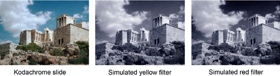
FIGURE 13.7. The conversion of a Kodachrome slide to monochrome with simulated yellow and red filters.
13.3 Polarization Filters
Polarization selection continues to be extremely important in photography, and its effects cannot be easily simulated in software. Understanding this phenomenon requires a consideration of the interaction of light with matter. For our purposes, light can be considered to be an electromagnetic wave with electric (E) and magnetic fields (H) perpendicular to the direction of propagation. The direction of the electric field defines the direction of polarization. The ray shown in Figure 13.8 is plane polarized (transverse magnetic, or TM), has the wavelength λ, and is propagating to the right with the speed c. The basic idea is that molecules tend to absorb light more strongly when their long axis is parallel to the direction of polarization. The effect is pronounced for molecules aligned in crystals, and the orientation dependent absorption is known as dichroism. In general, some kind of alignment of atoms or molecules is required for dichroism. Efficient and inexpensive linear polarizers are now available because of the insight of E. H. Land, the founder of the Polaroid Corporation.3
Unpolarized light consists of a collection of rays like that shown in Figure 13.8, but with random directions for their electric fields. In the following figures, I show only the electric field amplitudes since electric fields dominate absorption processes. Notice that in Figure 13.9 the electric fields initially lie in planes distributed around the z-axis. When the bundle of rays encounters the polarizer, the y-components of the electric fields are absorbed, and the x-components are transmitted. The result is a filtering process that passes an x-polarized beam. Figure 13.9 implies that the absorbing units are aligned in the y-direction. A perfect polarizer would pass 50% of the intensity; but, of course, there are reflections and other losses that limit the transmission.
Linear polarizers have been used successfully in photography for several decades, but with modern cameras problems sometimes arise from the interaction of polarized light with mirrors in the autofocus system and in the viewfinder. The efficiency of reflection depends on the state of polarization, and reliable operation may require unpolarized light. When it is desirable to take advantage of polarized light in a scene, there is a way to analyze for polarization and still insure that only scrambled polarization enters the camera. For this purpose, one uses a circular polarizer in place of the linear polarizer. The operation of a circular polarizer is illustrated in Figure 13.10. A linear polarizer selects the direction of polarization and then the polarized beam passes through a quarter-wave plate. The result is circularly polarized light in which the electric field vector rotates around the z-axis. The linear polarizer and the quarter-wave plate are actually glued together and act as a single filter. Within the camera, the circular polarized light acts like unpolarized light, and the problems vanish.

FIGURE 13.8. Polarized light with the wavelength λ.
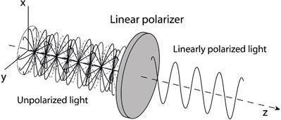
FIGURE 13.9. The interaction of unpolarized light with a linear polarizer.
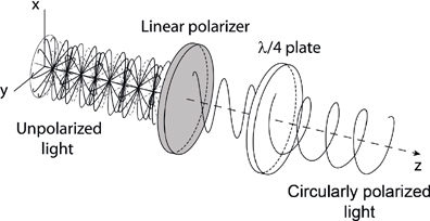
FIGURE 13.10. The interaction of an unpolarized beam of light with a circular polarizer.
So what is a quarter-wave plate? Here we encounter doubly refracting (birefringent) crystals such as calcite. These crystals are anisotropic, and the index of refraction depends on the orientation of the polarization of the incident light. It turns out to be possible to cut some birefringent crystals into slabs (plates) so that the directions of maximum (slow axis) and minimum refractive index (fast axis) are perpendicular to each other and parallel to the surface of the slab. The quarter-wave plate works like this. The birefringent plate is oriented so that the direction of polarization of the incident light lies between the fast and slow axes at to each. As shown in Figure 13.11 the electric field E of the light wave can be resolved into the components E1 and E2 that lie in the directions of the fast ands slow axes of the crystalline plate. Just as 2+2 is equivalent to 4 for integers, the sum of the component vectors E1 and E2 is equivalent to E. As I discussed in Chapter 6, the apparent speed of light in a transparent medium with refractive index n is just c/n where c is the speed of light in a vacuum, and the effective path length for light is the actual distance traveled multiplied by the refractive index. The quarter-wave plate is constructed by adjusting the thickness d so that the difference in path lengths for the components along the fast axis (refractive index n1) and the slow axis (refractive index n2) is one quarter wavelength or 90o phase shift. This is best expressed with the equation d (n1 – n2) = λ/4, which can be solved for the thickness if the refractive indices and the wavelength are known. The result is that two waves are produced, in perpendicular planes, that have equal amplitudes and are shifted in phase by a quarter wavelength, and it can be shown that the sum of these two waves rotates around the z-axis as illustrated in Figure 13.10.4
It has been suggested that polarizing filters can be stacked to “increase” the polarizing effect, i.e. to narrow the distribution of light that is passed by the combination (from cos2θ to cos4θ). This procedure will certainly fail for two circular polarization filters because the output of the first filter would be scrambled so that the second filter would not be able to improve the selection. Similarly, rotating one of the filters relative to the other would not change the fraction of light transmitted by the pair. The situation is different for a linear polarization filter before a circular polarization filter where distribution is indeed narrowed (to cos4θ). Also, rotation of one of the filters would attenuate the light completely when the filters were crossed. This combination could serve as a variable neutral density filter. Two linear polarizers would behave the same way, except the output from the second filter would not be scrambled.
13.4 Polarization in Nature
Photographers are interested in polarizers because they want to be able to control naturally polarized light as it enters a camera. Polarized light usually results from reflection or scattering. I first consider scattered light. This is not a simple topic, but a simplified model captures all the important features; and we only need two ideas to explain the phenomenon:

FIGURE 13.11. Resolution of polarized light into components.
1. The electric field of light exerts force on charged particles and, in particular, causes electrons in atoms and molecules to accelerate parallel to the direction of the field. These electrons oscillate at the frequency of the incident light wave.
2. According to Maxwell’s electromagnetic theory, accelerating electrons emit radiation. This is well-known from radio theory where current oscillates in antennas and broadcasts a signal to listeners. (Recall that acceleration is the rate of change of velocity. This naturally happens in an oscillation where the velocity periodically changes direction.)
These ideas apply to cases where there is little or no absorption, and the scattered light has essentially the same frequency as the incident light. Figure 13.12 shows the angular distribution of radiation for an oscillating electron. The distance from the origin to the red curve at a particular angle indicates the amount of light intensity in that direction. The important points are: (i) the direction of polarization is established by the direction of oscillation, and (ii) there is no intensity directly above or below the oscillator.
Consider, for example, a ray of sunlight in the sky, well above the horizon. It is easy to verify with a polarizing filter that the light exhibits very little polarization when one looks toward the sun or away from the sun. Maximum polarization is at 90° from the direction of the sunbeam, and the sky becomes quite dark as the filter is rotated. Figure 13.13 illustrates the situation. When looking toward the sun, we receive radiation from electrons oscillating in all directions that are perpendicular to the beam direction, but when the observer is in the plane of polarization all electron oscillation appears to be in one direction. When viewed from 90°, i.e. the observer is in the plane of polarization, the polarization may reach 75% to 85%. The polarization does not reach 100% because the oscillating electrons reside in molecules that are not perfect scatterers, i.e. the molecules are not perfectly spherical in shape and have a non-vanishing size; and, perhaps more importantly, some of the light is scattered by more than one electron before reaching the observer. Multiple scattering is the reason that light scattered near the horizon is not polarized.

FIGURE 13.12. The radiation pattern for a dipole radiator.
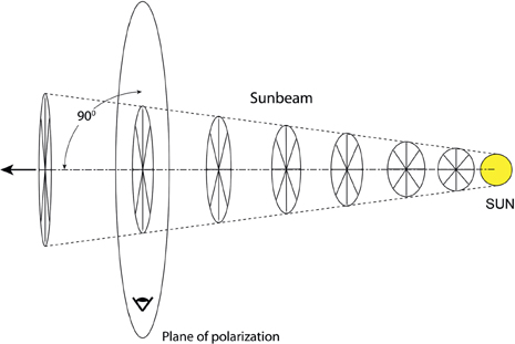
FIGURE 13.13. The transverse electric fields associated with unpolarized light from the sun.
Reflections are a major source of polarized light in nature. In the situations discussed here, light is reflected from a very smooth, nonconducting surface. (Surfaces that conduct electricity strongly absorb light, and the treatment presented here does not apply.) In such cases, the fraction of the intensity reflected depends on both the angle of incidence and the direction of polarization of the light beam. Figure 13.14(a) illustrates the reflection and refraction of polarized light with transverse magnetic fields (TM), which means that the electric fields are in the plane of the figure as indicated by the arrows (perpendicular to the scattering surface). In Figure 13.14(b) the incident beam is polarized with transverse electric fields (TE), meaning that the electric fields are perpendicular to the figure surface as illustrated by the x’s (parallel to the scattering surface). The indices of refraction above and below the reflecting surface are denoted by n1 and n2, respectively.
From previous discussions (Chapter 4) we know that the angle of incidence is equal to the angle of reflection θ1 = θ2), and the angles of incidence and refraction are related by Snell’s law (n1 sinθ1 = n2 sinθr). The physical description of reflection and refraction is as follows. The electric field of the incident light beam penetrates the glass/water interface and induces electric currents (oscillating electrons). The currents produce both the reflected and the refracted beams and cancel the beam in the direction of the undeviated dotted line. Notice that the electric fields of the three beams (I, A, B) are all parallel in (b), and we expect that the currents will produce reflected light regardless of the angle of incidence. In contrast to this, the electric fields of the three beams (I, A, B) are not parallel in (a). Since the oscillating electrons move in the direction of the electric field and do not radiate in the direction of their motion (Figure 13.12), it is clear in the TM case (part a) that no light will be reflected when the refracted (A) and reflected (B) beams are perpendicular.
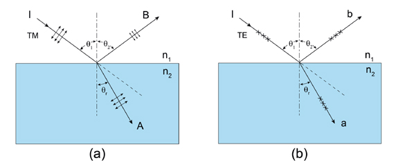
FIGURE 13.14. Reflection and refraction of light: (a) transverse magnetic field and (b) transverse electric field.
The remarkable conclusion is that, when unpolarized light is reflected from a smooth surface at one particular angle, the components polarized perpendicular to the surface are not reflected at all. At this angle, known as the Brewster angle, the reflected light is polarized parallel to the surface, i.e. out of the plane of the figure. Brewster’s angle can be determined by a simple calculation. [When paths A and B in Figure 13.14(a) are perpendicular, the angle of the refracted beam is given by θr = 90° – θ1. This expression can be combined with Snell’s law and the identity sin (90° – θ1) = cos θ1 to obtain n2/n1 = sin θ1/ cos θ1 = tan θ1.] The conclusion is that θ1 = tan–1(n2/n1). For example, a light beam in air that reflects from the surface of water (n = 1.33) at the angle tan–1 1.33 = 53.06°, or 36.94° measured from the reflecting surface, is totally polarized.
Of course, there is more to the problem than computing the Brewster angle. The percentage of reflected light from the TM and TE beams can be computed at all angles of incidence. This can be done by making use of simple geometric arguments or by applying Maxwell’s equations with appropriate boundary conditions to describe the electric and magnetic fields. The Maxwell equation approach, while more demanding, does permit reflection from absorbing material to be treated. Since these calculations would lead us too far afield, I simply present the results and provide references for the complete derivations. The fraction of light reflected for TM and TE arrangements is described by Equation (13.1).
![]() (13.1)
(13.1)
These quantities are plotted in Figure 13.15 for the special case with n1 = 1 and n2 = 1.33.
Polarization (TM/TE) at the Brewster angle (53.06°) is clearly shown, but it is also evident that polarization is strong from at least θ1 = 40° to 60°. The results are slightly different for glass where n2 ≈ 1.5. In summary, at glancing incidence (θ ≈ 90°) reflectance is close to 100% for both TE and TM components, and the reflected beam is not polarized. At normal incidence (θ = 0) about 4% is reflected with no polarization. Between glancing and normal angles there is some polarization, and it becomes complete at the Brewster angle.
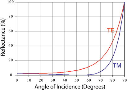
FIGURE 13.15. Percent reflectance for light at the air/water interface.
Polarization in a rainbow: Rainbows are favorite subjects for photographers, but few realize that the rainbow light is polarized. First, recall that rainbows are circles, and their center is always the shadow of the head of the observer, i.e. the anti-solar point. It turns out that the light from the rainbow is polarized tangent to the colored bands or perpendicular to a radial line from the center (see the yellow arrows in the photo in Figure 13.16). This happens because sunlight is reflected inside a water droplet and the droplet lies in the plane containing the observer’s head and the shadow of the observer’s head. Furthermore, the angle is close to the Brewster angle for internal reflection. The geometry of scattering is shown in Figure 13.16. Colors result from the dispersion in the index of refraction of water that ranges from 1.344 at 400 nm (blue) to 1.3309 at 700 nm (red), but reflection (inside water droplets) is responsible for the polarization.
A study of the possible angles for internal reflection, when there is only one reflection inside a droplet, shows that the maximum angle (from the anti-solar point) is 40.5° for 400 nm light and 42.4° for 700 nm light. This gives the primary rainbow, where the internal angle of reflection is about 40° and the Brewster angle is close to 37°. The secondary rainbow results from two internal reflections, and I find that minimum angle for 400 nm light is 50.34° and for 700 nm is 53.74°. In principle, the secondary rainbow has about 43% of the brightness of the primary, but it is almost invisible in Figure 13.16. The internal reflection angle for the secondary rainbow is about 45°—not quite as close to the Brewster angle as with the single reflection. The consequence of the limiting reflection angles is that the colors are reversed in the secondary rainbow going outward from red to blue, and that no light is reflected between roughly 42° and 52° by either single or double reflection. This gives rise to the dark band between the primary and secondary rainbows that was described by Alexander of Aphrodisias in 200 CE. and bears his name. Rainbows also result from three, four, and higher numbers of reflections in droplets. The tertiary rainbow appears as a ring around the sun at 137.5° and is extremely difficult to see. Higher order rainbows up to order 200 have been seen in the laboratory with laser light. Additional discussion and illustrations can be found in the book by Lynch and Livingston (see Further Reading).

FIGURE 13.16. Refraction and reflection of light beams in rainbows: (a) primary and (b) secondary.
Reflection by metals: So far I have limited the discussion to reflection from nonconductors. The problem with conductors of electricity is that they absorb light and, in some cases, absorb very strongly. Actually, the stronger the absorption, the higher the reflectivity, and the reflectance can reach nearly 100% without any polarization for polished metals. More poorly reflecting metals such as steel partially polarize reflected light. For a typical metal, reflectance of both TM and TE beams depends on the angle of incidence, and the TM beam shows minimum, though nonzero, reflectivity at the “principal angle of incidence.” There are no universal polarization curves for metals since the reflection of polarized light depends on the optical absorption coefficient, which in turn depends on the wavelength of the light. Photographers must depend on trial-and-error methods with metals.
13.5 UV and IR Photography
The human eye can only see a very narrow band of radiation between about 400 nm and 700 nm that is defined as the visible region. Thus, we are restricted to a region of the electromagnetic radiation spectrum where the frequency varies by only a factor of two. At first glance that seems remarkable, since the complete spectrum from gamma rays to radio waves encompasses almost 15 orders of magnitude change in frequency. However, humans evolved the ability to see sunlight; and most of the energy from the sun lies in the visible region. The solar flux is illustrated in Figure 13.17. At wavelengths less than 400 nm, where the UV-A region begins, the intensity of the solar spectrum decreases, and it is severely attenuated below about 320 nm because of absorption by ozone in the atmosphere. This loss of intensity is a very good thing since photons in the UV region have high energy and can damage skin cells as well as the photoreceptors in the eye. In the infrared region beyond 700 nm there is still considerable intensity, but the photons have low energy and the photoreceptors in the eye are not very efficient at their detection.
Obtaining UV images: So we accept the fact that human vision is not good in the UV and IR regions, but what about photography. First consider the near UV region (320–400 nm, UV-A). The major problem we encounter is that glass in standard lenses begins to absorb light at about 420 nm and by 370 nm transmits very little. Practitioners in UV photography use special quartz/fluorite lenses that transmit UV at least to 300 nm. The UV-Nikkor 105 mm lens is often mentioned, and the Jenoptik CoastalOpt 60 mm f/4 Apo Macro is a special purpose lens that covers the region from 310 nm to 1,100 nm. Both of these lenses are extremely expensive. Some commonly available lenses transmit light well beyond 400 nm and permit amateur photographers to experiment with near UV photography. The best candidates are simple lenses without cemented elements and without optical coatings, and adapted enlarger lenses also have been suggested.
The next thing that is necessary for UV photography is a filter that can completely block visible light. The Kodak Wratten 18A transmits from 300 nm to 400 nm and blocks visible light, but it also transmits IR from 700 nm to 900 nm. Other UV transmission filters such as the B+W 403, which are less expensive, have the same IR problem. There are better but much more expensive UV pass filters. The Baader U filter transmits UV light in the region 320–390 nm and otherwise blocks the region 220–900 nm. Also, LifePixel and other companies offer UV-specific camera conversions.
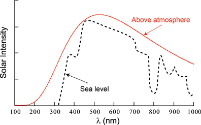
FIGURE 13.17. Sketch of the solar intensity versus wavelength above the atmosphere and at sea level.

FIGURE 13.18. Paul Green Cabin: Canon G-1 camera (a) without filter and (b) with B+W 403 UV pass filter.
Finally, one needs a sensor that can detect UV. CMOS sensors in most digital cameras turn out to be satisfactory. It is even possible to obtain interesting results with some standard lenses and some experimentation. As an example, I show images obtained with a Canon G-1 camera with and without a B+W 403 UV transmitting filter (Figure 13.18). As noted, the filtered image is contaminated with IR radiation. The UV image was brightened with Photoshop, but the false colors were a surprise. It is fair to say that UV spectroscopy is not of much interest to amateur photographers except maybe in astrophotography. The important uses of UV photography include dental imaging, skin damage analysis, and the recovery of evidence in forensic science.
Obtaining IR images: Fortunately, IR photography is fairly easy and often rewarding for amateurs. Although film with IR sensitivity is increasingly difficult to find since Kodak discontinued production, Rollei and Efke IR films may still be available. Lenses are not a big problem in the IR. Many standard lenses are satisfactory for IR photography. The problem, when it arises, is that some lenses give “hot spots” in IR photographs. Also, the focus scale shifts and some lenses lose resolving power especially at the edges. One must select lenses by trial and error. There are also lists of lenses that have been found to be satisfactory, but I find some of the recommendations not completely accurate. Some high quality lenses fail to give corner-to-corner sharpness with IR light.
Of course, filters have to be used to block visible light, and here there are a lot of choices. One has to decide on the desired cut-off point. Some popular filters are listed in Table 13.2. Many other filters are available, and equivalent filters can often be obtained from B+W, CoCam, Cokin, Heliopan, Hoya, Schott Glass, and Tiffen.
In digital photography we must deal with CCD or CMOS sensors in place of film. These sensors are inherently sensitive in the red/IR region, so much so that without blocking ambient IR the recorded colors may be distorted, i.e. IR will be will falsely recorded as a visible color. Therefore, manufacturers have installed hot-mirror IR reflectors to prevent IR radiation from reaching the sensors. Of course, the hot mirrors are not perfect and some IR gets through. So we add a filter to block visible light and hope that enough IR gets through the hot mirror to permit an image to be recorded with a reasonable exposure time. As you might guess, some cameras are accidentally better than others at producing IR images this way. As an example, I used a Canon G-1 (3 megapixel) with a Hoya R72 (Wratten 89B equivalent) on a tripod to photograph Mabry Mill on the Blue Ridge Parkway. Figure 13.19 shows this photograph compared to one taken (hand-held) without the IR filter. Both were converted to monochrome in Photoshop. The obvious differences are in the foliage, which is white in the IR photo, and the water, which is black in the IR photo. Blue sky would also be very dark in an IR image, but in this case there were thin clouds. In general, IR images are more striking than ordinary black and white, and it is possible to obtain very interesting false color images. Even though the exposure time was very long for the IR shot, the experience was not bad because the image was clearly visible on the LCD screen even though the filter looked quite opaque.
TABLE 13.2
Red and IR filters
| Kodak Wratten filter | 25 | 89B | 87 | 87c |
|---|---|---|---|---|
| 0% Transmission (nm) | 580 | 680 | 740 | 790 |
| 50% transmission (nm) | 600 | 720 | 795 | 850 |
Of course, action photos are out of the question with long exposures, and even a breeze can upset things by moving leaves and branches. The way around this problem is to have the IR filter (reflecting hot mirror) removed from the digital camera. Several companies offer this service now for both point-and-shoot and interchangeable lens cameras. There are two options. The IR filter can simply be removed, and the user then must use an external filter for normal photography and a visible blocking filter for IR photography. The downside of this arrangement for DSLRs is that one cannot see through the dark IR filter and must remove the filter to compose the scene. The other option is to have the IR blocking filter (hot mirror) in the camera replaced with a visible blocking filter mounted directly on the sensor. There are more possibilities here because the available blocking filters range from 590 nm (super color) to 720 nm (standard IR) and even to 830 nm (deep IR). The LifePixel website offers useful tutorials about filter choice and image processing.5

FIGURE 13.19. Mabry Mill: Canon G-1 camera (Upper) without a filter and (Lower) with a Hoya R72 IR filter.
With filter replacement, the camera works normally and is even convenient for action photography. The IR conversion is an attractive option for a camera that has been replaced with a newer model. There is, however, a change in the focusing scale that requires compensation unless focusing is based on the image at the sensor. This is not a problem for DSLRs in Live View mode or for mirrorless cameras. Companies that advertise IR conversions include LifePixel and MaxMax.
The images shown in Figure 13.20 were obtained with an 18 megapixel Canon SL1 (100D) camera that had been converted to IR by LifePixel. A 590 nm filter was chosen so that some color information could be retained. The images were taken at midday with a wide-angle lens (1/320 s, f/10, ISO 200). Processing of the black and white image consisted of minor adjustments to exposure, contrast, clarity, and sharpness followed by conversion to monochrome in Lightroom. The work flow for processing of the color image was more involved. First, the white balance was adjusted either with Canon Digital Photo Professional software or with a custom camera profile in Lightroom. The image was then exported to Photoshop so that the Channel Mixer could be used to switch the blue and red channels to get blue color into the sky. The positions of the red, blue, and green color sliders are arbitrary and are set according to the photographer’s preference. Recommendations about IR image processing can be found in LifePixel tutorials and Bob Vishneski’s website.6

FIGURE 13.20. Point Reyes shipwreck IR image rendered in black and white and in color.
Further Reading
Feynman, R. P., Leighton, R. B., and Sand, M. (1963). The Feynman Lectures on Physics, Vol. I. Reading, MA: Addison-Wesley, Section 33-3; Vol. II, chap. 33. A discussion of polarization for students of physics.
Fowles, G. R. (1989). Introduction to Modern Optics, 2nd Ed. New York: Dover Publ. A good modern optics text.
Land, E. H. (1951). Some Aspects of the Development of Sheet Polarizers. Journal of the Optical Society of America, 41(12), p. 55. Dr. Land discusses the history of polarizers.
Lynch, D. K. and Livingston, W. (2001). Color and Light in Nature, 2nd Ed. Cambridge: Cambridge University Press. This is a beautiful and fascinating book.
Notes
1.Filters have a long history in photography. The earliest photographic emulsions were primarily sensitive to blue and UV light, but in the 1870s the German photochemist and photographer Hermann Vogel learned how to extend the sensitivity into the green region by adding dyes to silver bromide. The result was the orthochromatic plate, still lacking sensitivity to red light. Adolph Miethe, an astrophotographer who succeeded Vogel as Professor of Photography at the Royal Technical University in Berlin, was able to extend sensitivity to the complete visible spectrum in 1903 to produce panchromatic emulsions through the addition of the sensitizing dye, ethyl red. However, there was still excessive sensitivity in the blue region, and realistic tones could only be achieved by photographing through a yellow filter.
Photographic filters that selectively attenuate colors were invented by Frederick Wratten for dealing with the limited tonal ranges of available emulsions. The ability to modify tones in black and white images became very important to photographers, and in 1912 Eastman Kodak purchased Wratten’s company and continued the production of “Wratten” filters. Later, after color emulsions became available, filters were even more important. Each color emulsion was designed with a particular white balance. For example, film for daylight use might be balanced for 5500K light. Such an emulsion would produce a decidedly yellow-orange cast if used with tungsten incandescent light (3400K). The way around the problem was either to purchase a film balanced for 3400K light or to use a blue filter (Wratten 80B). Conversely, “tungsten” film balanced for 3400K could be used in daylight by adding an amber filter (Wratten 85).
The introduction of digital cameras along with computer post-processing of images has drastically reduced the need for colored filters. These cameras have built-in UV and IR filters to avoid false colors, and the white balance can be set in the camera or (in some cases) postponed for later processing. Overall attenuation to permit long exposures is still desirable, and selection of the direction of polarization remains an important option. In addition, ultraviolet (UV) and infrared (IR) photography require that visible light be blocked with a filter.
2.Unfortunately, Bouguer did not get full credit for the absorption law because he did not provide a compact mathematical expression to describe the effect. Johann Lambert’s contribution was to apply the calculus to sum up the contributions of infinitesimally thin layers to show that the attenuation decreases exponentially as described by the equation I/ I0 = 10–OD where OD is defined as the optical density. [Actually, Lambert’s expression was closer to I = I0exp(–a • l) where a is a constant that denotes the absorption coefficient of the material and l is the thickness of the sample. There is a simple conversion between the forms of the equation, given by OD = a • l/ln(10).] So how did August Beer get into the act? His contribution was to relate the OD, or absorbance as chemists call it, to the concentration of particles or molecules in a transparent liquid solvent or perhaps the atmosphere. Thus, in place of Lambert’s constant a, Beer introduced the product of a molar absorption coefficient and the concentration of the particles. This turned out to be very important for chemists because, given the molar absorption coefficient, the concentration of a solution could be determined from a measurement of the optical density (or absorbance).
3.Some forms of crystalline tourmaline are naturally dichroic so that one crystal will polarize light and a second crystal can be rotated to totally block the polarized light. However, tourmaline absorbs light too strongly to be used as a practical polarizer. Crystals of herapathite (quinine sulphate periodide) were also found to be dichroic in the nineteenth century, but it turned out to be very difficult to grow the crystals large enough to make useful polarizers. In spite of that, Carl Zeiss was able to market “Bernotar” single crystal herapathite polarizing filters for photography. Information about the crystal growing techniques they used was apparently lost in World War II.
Commodity polarizers date from the 1920s, when the scientist/inventor Edwin Land demonstrated that a suspension of tiny crystals (ground in a mill) aligned by electric or magnetic fields can also polarize light. With the insight that aligned crystallites or even aligned molecules can substitute for a single crystal, he went on to develop polarizing sheets of PVA (polyvinyl alcohol) doped with iodine atoms. The trick was that the sheets were stretched in the manufacturing process in such a way that the polymer molecules were aligned and the attached iodine atoms formed chains. The chains of atoms act like short segments of metallic wire that strongly absorb light polarized parallel to their length. It is the electrons, that are free to move in the direction of the atomic chain, that interact with the electric field With this technique and various improvements, Land’s company, Polaroid Corporation, was able to produce efficient and inexpensive polarizers for sunglasses, photography, and a variety of other uses.
4.Suppose that polarized light with the maximum amplitude E and the intensity I (Figure 13.11) is incident on a linear polarizer so that the component E1 is transmitted and E2 is blocked. The transmitted light has the amplitude E1 = E • cos θ and the intensity is I1 = I • cos2θ. If the incident light is unpolarized, the angle θ is distributed over 360°, or 2π radians, and one must obtain an average of cos2θ in order to compute the intensity of the transmitted light. The result for the transmitted intensity is Ipolarized = I/2. This explains why 50% of unpolarized light is transmitted by a linear polarizer.
The expression for the circularly polarized light is more interesting. At an instant in time, say time 0, the amplitude of plane polarized light varies according to position on the z-axis (see Figures 13.8–13.10). For the x-component the amplitude is described by E1 = cos(k • z) where k = 2π/λ. If the y-component is represented by E2 = cos(k • z) with E1 = E2 then the result is just a linearly polarized wave at 45° as shown in Figure 13.11. However, the introduction of a quarter-wave plate changes things so that the y-component becomes E2 sin(k • z) and the resultant rotates around the z-axis. Note that a quarter-wave plate requires no filter factor because the electric field of the light beam is not attenuated. In fact, a second quarter-wave plate (rotated by 90°) can be used to restore the original linear polarization without loss. The x-and y-components shown here were used in the program Mathcad to generate the sine curves in Figures 13.9 and 13.10 and the helix in Figure 13.10.
5.https://www.lifepixel.com/tutorials
6.https://photographylife.com/how-to-process-infrared-photographs#comments