Clarifying Terminology

At this point, I want to present a short, three-character terminology clarification to avoid confusion or uncertainty. We will use these terms in the same way as they were introduced in Chapter 4 of Google’s Site Reliability Engineering book.

Establishing SLAs for Internal Components

What if the service is not an end-customer-facing one. Should it have its own SLA, too? To clarify the “Yes” answer, let’s play with an imaginary message distribution service (see Figure 9-1) that consists of the following four main components:

Data receiver

Accepting and registering messages

Data transformer

Adjusting message content with data from separate external sources

Distributor

Delivering messages to multiple endpoints

Consumer

Receiving data from the endpoint over a “publisher–subscriber” model

Figure 9-1. Message distribution service components relationship

At the moment, this system is working fine: no errors, no alarms.

One day, one of the top project managers comes to us and poses the following: “One of the projects we are working on now uses the ‘message distribution service.’ From time to time, we will need to send a huge amount of data in a short time period. Can we use this service as it is, or how should we adjust its capacity in order to handle the new traffic?

Let’s work this out gradually. Having an actual number for the data amount is handy. Let’s say that the forecasted traffic will be three times higher than the maximum known peak-time value. However, this knowledge will not provide us with a clear understanding of whether we will be able to handle such growth. The reason is simple: even if we know how much data is managed by the service right now during peak times, we would still need to know the breakpoint at which we reach the service’s capacity limit to be able to compare it with the forecast.

Our message distribution service has several components. The slowest component is the one that dictates overall service capacity: the “strength of the chain is determined by the weakest link.” So now we need to spend some time to establish a performance-testing environment and identify breakpoints² for every component separately and determine which component is the bottleneck.

So far, we have data that will tell us about traffic-handling possibilities: the number of messages that can be consumed without errors. And if it is fine, we are ready to go on to announce that no changes are required. That would be a great scenario if we had planned such growth in advance. Otherwise, if we can serve three times more traffic without rescaling, and service consists of more than one host (undividable resource unit), it might mean that up until now two-thirds of all allocated resources were never used, which might raise a question about cost efficiency. But that is a different story, and hopefully it is not the case.

Comparison of the test results and the forecast reveals that we can deal only with half of the expected growth. And we now, as per the new request, need to at least double throughput.

This is a relatively simple task. Traditionally, to solve such a problem SysAdmins determine the critical system resource—like CPU, memory, disk, network I/O, and so on—that is used the most, and that is the one that actually needs to be doubled. Then, they accordingly request new hardware to cover necessity. And there is nothing wrong with this approach. However, there is something else that is lying outside of its scope and hence not counted.

From the SRE point of view, we were missing additional service-specific restrictions without which we cannot scale our service accurately.

For our imaginary service, the goal is to pass a number of messages throughout from the entry point to the final consumer in a reasonable amount of time. Each component has only a limited time that it can stay inside each component before it will be sent to the next component. And this is our specific restriction: the time limit per component. Without such a limitation, during the traffic growth, some messages can be delayed or stuck for a very long time somewhere in the middle. This problem would not be visible; delayed messages are not marked as problematic because they do not raise any errors. They don’t raise errors just because we don’t know what duration is “good” and what isn’t.

To overcome this inconvenience, we should express the overall delivery time in a particular time value. Then, we should assign the portion of it to the specific component and, again, define it in the exact time value. Here, we are correcting the meaning of a breakpoint for the performance testing procedure. What we need is not the number of messages that we can receive without errors, but how many messages this component is able to pass through such that every message been processed for no longer than the defined time limit. Establishing these limits usually decreases the previously calculated capacity even further.

Time constraint per component is nothing but another SLI (“Passing time”) and its value is determined for every component individually. Also, each component has other valuable indicators such as “Availability” and “Response time.” When combined they form a per-component SLA.

Now we have an SLA of two natures. The first is the one that we mentioned earlier, which covers the entire service and is exposed to the services’ customers. We will use it to observe the overall service behavior.

The other one is the per-component SLA. It is not presented to the services’ end users; however, it allows us to determine the relationship between components, helps to identify quickly which component caused difficulties to the overall service, and is used to precisely scale the component. Its SLI’s values can (and should) be used during performance testing as limits to identify the correct breakpoint.

For our toy service, the breakpoint will be identified as a maximum throughput at which a component will meet the following demands:

• 100% of requests get responses faster than the certain limit.

• No errors occurred.

• 100% of messages are sent to the next component such that every message met its time limitations.

Keep in mind that all three criteria must be verified simultaneously, because receiving messages and sending them further might be done asynchronously by different processes, and the good condition of one metric does not mean the same status of the other.

Back to our scaling. We previously said that we need to double the throughput. Now, this statement needs to be revised because we changed the testing procedure by appending new requirements, and the results might not be the same as before.

The forecasted input will be received by the first “Data receiver” component. Knowing particular values of expected traffic and component performance metrics, we can finally estimate required capacity adjustments. We can calculate the potential maximum capacity we have now, the required capacity that can handle the maximum traffic expected, and then find the delta between the two. But this will be true only to the “Data receiver” because the forecasted input defines the size for this component only.

Do not forget that, for instance, doubling the throughput for a component does not necessarily mean that we need to double its fleet. Not all components scale linearly, so for some of them, it will be enough to add only a few machines. For others, it might require adding much more than double the number of hosts.

But what about the next component? In the same way, we can calculate its current capacity, but we don’t know how much data it will receive from the previous one. We can assume that its traffic will increase according to the growth of the previous component’s input, but this would be only an assumption, which might have nothing to do with reality.

Knowing what a component does, we can perform a set of experiments that will establish a ratio between the input and output of the component.

Now we can approximate the amount of input data for every individual component from the originally forecasted amount. For example, if the input/output ratio for the “Data transformation” component is 1:2, and 1:1 for the “Data receiver,” it means that for every original megabyte of messages, the “Distributor” will get two.

Before we move on, we should say a few more words about the bottleneck component. We keep track of it for a single reason: the bottleneck is the first component that will experience difficulties in case of traffic growth. In other words, if this component is overloaded, the entire service has a problem. Why do bottlenecks exist if we scale every component to the maximum performance and throughput needed?

There are two factors. The first is that some components will be a bit overscaled. For example, if a single host can handle 1 million messages per minute, but the traffic is 1.1 million, adding the second host will leave 90% of its capacity (or 45% overall) unused. And this component will be fine until traffic reaches the 2 million messages per minute rate. But the other part of the service, in contrast, may already utilize its capacity up to 95% processing the same 1.1 million messages. The second factor is the input/output ratio. If for the first component the growth of incoming traffic is small but the rate is high, the input to the next component might increase significantly and might require our attention.

The bottleneck is the component that in comparison with others has minimal difference between current load and maximum available capacity, is very sensitive to traffic changes, and is the first that will be overloaded.

Returning to our story, to illustrate how the bottleneck identification works, let’s imagine that the forecasted load peak is 1,000 RPS; the components’ capacity after rescaling is as follows:

• Data receiver: 1,300 RPS

• Data transformer: 1,250 RPS

• Distributor: 1,100 RPS

With this information, we now have located a bottleneck; it is the Distributor because its performance is closest to the forecasted peak and, in spite of the Data receiver capabilities service, will work fine only until the load is less than 1,100 RPS. The next bottleneck is the Data transformer because it is the closest component to the current bottleneck, and so on.

So far, we know the following:

• Where the bottleneck is. And we can predict where the bottleneck will relocate from where it is now (literally this means that now we know the next slowest component, the next after that one, and so on).

• Expectations for every component (number of messages that can be processed by a single application instance and the expected amount of time that message can spend inside this component—literally an SLA).

• Per-component incoming/outgoing traffic ratio. We can predict the traffic volume between components and fit capacities accordingly.

• The overall and per-component capacity and how much of it is actually in use. We are also able to predict capacity drops in case of a variety of outages and make resource reservations accordingly.³

Our scaling calculations are based on the forecasted values. Keep in mind that the real traffic can have different characteristics. Continuously tracking available capacity along with the knowledge of whether all components stay within their SLAs will clearly tell us how “good” our service is doing.

The real-world scenario can become more complicated. There might be more than one SLA per service because we might have several data types, and each of them might need to be treated differently (Figure 9-2). In our case, different messages might have different priorities and processing-time restraints. Without an individual SLA for each priority, it would be tough to say what we should do if there is a growth in the load from only one of the data types even though this might affect the others.

Figure 9-2. Components relationship in terms of SLAs and traffic patterns for two message types

Here’s a short example: due to high load spikes in high-priority messages, other message deliveries will be slowed down from a few seconds to several minutes. The key question then is, is a delay of several minutes acceptable?” By applying the “divide and conquer” principle, we declare specific criteria for every type separately, and if we know exact barrier values and can quickly identify “good” and “bad” values, there will be no problem taking the right action. Otherwise, we will fall into a state of not knowing and can only guess what to do or whether we should do anything at all.

Establishing SLAs for internal components helps to clarify the relationship between them and precisely coordinate their interaction. This is true not just across components but also across big services. SREs mostly focus on service efficiency and quality tracking what matters to the user. Service architecture and particular applications used are secondary, at least until a service delivers results according to a user’s expectations.

And this is still not the end of the story!

Understanding External Dependencies

As you might recall, the “Data transformer” component in the course of its work adjusts messages’ content with information from separate external sources. These sources are called external dependencies. The difference between a dependency and the services’ components we have been discussing up to this point is that as opposed to a component, we cannot control a dependency and its behavior. Here, “Data transformer” is playing the role of a customer, and these external services are just a set of “black boxes.”

From this perspective, the question is, “What capacity can these external services provide and how will their limitations affect our component’s performance and scalability?” We want to know what we can expect, and, technically, we are asking for an SLA. We need this to understand whether we can use the service as a dependency, or we need to look around to find another solution for our task. The provided SLA will give us a clue about available limitations (like request size), performance (like response time), and availability, but still, how is our component performance affected by this and does it suit our needs?

If we imagine that we are SysAdmins who care mostly about service health and load and have nothing to do with SLAs—which, by the way, may not exist at all—the question we asked will be very tough to answer. However, knowing precise requirements for our own service (while we change our point of view closer to an SRE perspective), we can easily compare the values between SLAs that will direct us to the answer. Let’s see. If, for example, the requirement to pass a message through the Data transformer component is 50 ms and we spend half of this time on internal manipulations only, we have 25 more milliseconds that we can designate to requesting data from the external source. By having an SLA for that source that states the response time should be less than 20 ms, we can confidently say that it is safe to use this service as a dependency.

As another example, it might be a stated capacity limitation that the dependency could serve only 900 RPS per customer account, and if the previously discussed 1,000 RPS of the forecasted peak value is still applied, we will either need to ask to raise the limit or to look for another solution.

The final case worth mentioning is when the performance of the dependency dictates our own component throughput. Suppose that without dependency the Data transformer can process 2,000 requests per second. If the performance of the external source is 1,100 RPS, the Data transformer will be limited by its performance to the same amount of 1,100 RPS. We’re definitely able to use this service as it is, but we should keep in mind that the performance of our component is limited not by its own performance or capacity, but by the external dependency capabilities. This is a very important point because if we, someday, will need to scale up throughput of the Data transformer higher than 1,100 RPS, changes on its capacity will not make sense.

As is demonstrated here, we now can not only say whether we can use this service, but we’re also able to predict whether we will reach the dependency’s limits and if so, in what circumstances it would happen.

Another aspect of the external dependency is the tightness of a relationship between our component and this service—in other words, how an external service outage will reflect on our component performance and availability. To demonstrate the meaning of tightness, let’s look at a couple of examples.

The most widely used external dependency is Domain Name System (DNS). If a component is frequently resolving domain names, an outage of the DNS might paralyze it completely and the entire service will be affected. The less expected scenario is when only a part of the service experiences difficulties. The entire service can also be affected, but this time it might be a bit more difficult to trace the source of a problem.

For the second example, we will discuss a less frequently used service called Lightweight Directory Access Protocol (LDAP). If we assume that the service calls LDAP only a few times during the start, the only moment during which our component can potentially be affected is while the service is starting or restarting.

Overall, the tightness of the relationship between the component and LDAP service is very low compared to the one between the component and DNS. Both services can affect their dependents, but the severity of a failure event is significantly different.

To visualize a dependency relationship, let’s make a list of all of the external services we are using along with their SLAs and potential outage effects. Having it readily at hand in an emergency such as a fire could be critical. It could save you many priceless minutes that otherwise would be wasted figuring out influences on the fly. You should update it every time you add a new major feature or a new dependency.

From the SLA perspective, we need to make sure that our service’s promised level of reliability is not higher than the lowest level among all direct dependencies. If we noticed that this might be the case, we need to either downgrade the SLA or find a technical solution to mitigate the difference. For that purpose, in some cases, we might develop a thin intermediate layer with, for example, caching or replication. Keep in mind that we may compare only directly related dependencies and that the service is depending not only on software, but also on hardware, power supplies, a network provider, and so forth, and they all have their own availability limitations that can affect us.

Even at this point, the understanding of whether the service is okay heavily depends on a personal point of view. The outage of a single dependency that blocks part of the service will be treated as a big problem by the classic SysAdmin role, but for SREs this service might appear to be only partially affected or even totally fine. For our messaging case, an outage of the “Data transformation” dependency might block this component entirely (service outage for SysAdmins). But even if we still can receive new messages and store them for a while, the high-priority messages would be affected immediately in terms of delivery timing. However, the low-priority traffic might not be affected at all (for SRE, service is only partially affected). Moreover, if there is no high-priority traffic at the moment, the service is totally fine (unless we are not breaching delivery time limits for the low-priority messages).

Now we see how the new viewpoint can dramatically change the way we understand the current service condition. Interestingly, when we actually write down the ideas of what we expect from a service and begin to collect related data to measure what we have in reality, it usually turns out that the service is not doing as well as we believed it was doing.

Measured results are different because, without an SLA, we can count only these problems that somebody complained about. And in our mind, the service is doing well because there were only a few complaints in the past that appear to have been successfully resolved. The problem is that we did not receive complaints about all of the issues we actually have and, in reality, there might be a thousand cases in which end users just leave silently with a bad taste in their mouth.

Nontechnical Solutions

Technical solutions are not the limit of an SLA’s potential. SLAs will give you a hand in other fields as well. The SLA determines, for instance, the right time to hand a new service over to the SRE team to support. This can be as simple as, “If a product meets expectations (i.e., does not violate an SLA), the product is ready; otherwise, it is not.”

When we talk about the handover procedures, the first thing that comes to mind is a big checklist with dozens of bullet points. It covers all possible aspects of the service, from architecture decisions and comprehensive administration documentation to monitoring alarms and troubleshooting runbooks. However, having all these bullets checked hardly gives you a strong sense of confidence that it is ready to be taken over. Unless you are freezing all activities except transition preparations, that is a very unusual thing to do; you will never be 100% sure that there will be no unpleasant surprises.

Consider the following. All new software projects will have some prerequisites long before they pass architecture review and a couple of proof-of-concept models have been built. When it is believed that an application is ready to be officially launched and begin serving live production traffic, both SLA and SLO counters are reset⁴ and start to collect the real data. This is the starting point for the service condition measure. Because the SLA defines statements over time (the frequently used period is one calendar year), the project should last in this state a significant portion of this time (several months or a quarter) to collect enough data points that confirm that the service is stable enough and that there are no agreement violation risks.

If we add an “expectations reaching” goal as an additional checklist point along with the alarms limitations (amount of alarms for a service during the time period; e.g., “No more than one alarm per two weeks”), we will be much more confident that service was not on fire for long enough before, that it is not on fire now, and that the developers team is able to maintain this state and it will not throw you a curveball.

Similar to this example, you might put any task or idea through the SLA prism to see how impactful it is for your customer and treat it accordingly. This understanding will guide you not only about the points that need to be improved, but also about where further improvements are unnecessary and therefore you can switch your attention to something else. As an example, if your SLA stated the requirement of 99.9% availability, but for the last quarter the service is running as good as 99.999%, you do not need to do any more work on that service.

Now, let’s see how theory meets with practice.

Tracking Availability Level

All right, so let’s assume that we’ve successfully defined an SLA. But from a practical perspective, how should we track all of these numbers and percentiles?

Before jumping into the arithmetic, let’s clarify some meanings first.

Here, we need a list of all agreement violation conditions to take them all into account. Let’s name these conditions as “failures” to distinguish them from the “errors” we have been using previously. This separation is necessary to stress that we will not use these two terms interchangeably. Failures will contain not only errors, but also a variety of other events that, one way or the other, affect the availability metric. Moreover, the spectrum of included errors also needs to be restricted, because the “404 Not Found” HTTP error, for example, is more of notification rather than an actual error caused by service internals and hence should be removed from the list.

To return to our previous example, let’s say that for the high-priority traffic for the “Data receiver” component of the “Messaging bus” service the SLA is defined as follows:

We will process all messages marked with the high-priority flag within 10 ms in 99.9% of cases over a calendar year.

The list of failures, in this case, will contain the following:

• Messages that took longer to process than 10 ms.

• Messages unable to be processed due to internal service problems but not caused by incorrect incoming requests.

To track the ongoing availability level, we need to subtract the number of failures from the total amount of messages received.

So, let’s run the math. Our initial availability is equal to 100%. After the first 24 hours, we will collect all metrics, calculate a number of failures, and finally get the new availability value to start the next day with it.

If for the last day we receive 1 million messages and 200 of them were marked as failures for whatever reason, the availability would be reduced to 99.98%, calculated as follows:

100% – (200 / 1,000,0000 × 100) = 99.98%

This calculation method will work fine to a certain extent, but it does have a few problems. The first one is that availability level changes in only one direction and once decreased will never recover.

The second is that we do not take the “over time” distribution into account, which can lead to dramatic drops where it is not expected at all. For instance, suppose the traffic is served by two hosts fronted by a load balancer and there was a very quiet time period during which only 10 messages were sent for an entire day. What would happen to the statistics if one of the hosts begins producing errors for every received message? If all 10 messages were sent back to back, they were equally spread between the hosts and half of them failed. The load balancer resent them to the other host and finally all 10 were successfully delivered. From the calculation perspective, it would be a huge availability drop:

100% – (5 / 15 × 100) = 66.67%

A 33.33% drop without any customer impact!

The last obvious constraint is that we are unable to plan maintenance that requires downtime because it is unclear how to integrate this intentional downtime from the messages amount perspective.

This leads us to another difficulty: unsafe update rollouts. Any rollout with massive changes can potentially end up counting as an entire service outage regardless of the number of tests and canary⁵ stages the software passed. The problem is not the outage by itself; the problem is our inability to predict in advance whether such events will break the SLA. Even if we know how much time we need to detect an issue and perform a rollback, it is still unclear how to compare this time with the available 0.1% of cases that are left apart from that 99.9 % that we agreed to serve correctly.

The solution is hidden in the interpretation of the “99.9% cases per year” statement. The “year” is a value of time, and thus 99.9% can also be treated as a time value.

According to this statement, we can count how much time per year we have left for failures and maintenance. A single year consists of 525,600 minutes. The 0.1% that is left beyond the SLA level is equal to almost 526 minutes. Google gives this value a unique name, the error budget. The percentage of time that service worked correctly over the year is usually referred to as a service’s “uptime,” and “99.9%” specified in the SLA is the acceptable level of this metric.

Literally, we can interpret the error budget as follows: if the service does not produce even a single failure for the last 365 days, we can shut it down completely for about 8 hours and 45 minutes without violating the SLA.

Now we are able to compare rollback timing requirements against such a budget to see whether the next rollout will put availability levels at risk.

Also, availability level (uptime) now becomes recoverable. Previously, we were able only to decrease the uptime value, but the new method allows us to restore it over time up to the original 100% mark. Because “a year” is a constant duration value, every new minute of operation appends new metric values into the head of a year timeline and discards the same amount of data from its tail. If we calculate availability on a daily basis, every time we will work with 1,440 minutes of data. By subtracting all of the failure time from 1,440 daily minutes, we get a “daily uptime.” To calculate new overall service availability, we need to subtract daily uptime as it was a year ago from the previous overall availability value and append it with today’s uptime. For example, if we have the following:

• Yesterday’s service availability level: 525,400 (99.9619%)

• Error budget size: 326 minutes

• Daily availability for the same day last year: 1,400 minutes

• Today’s failures: 5 minutes

Today’s overall uptime is as follows:

Uptime = “Yesterday’s uptime” – “Last year’s daily uptime” + “Today’s daily uptime”

525,400 – 1,400 + (1440 – 5) = 525,435 (99.9686%)

Here is the current error budget calculated as a difference in minutes between the current overall uptime and the SLA level:

525,435 – (525,600 – 526) = 361

As we can see, last year we had only 1,400 minutes of correct operation, which means that the 40 remaining minutes were used by failures and cut off from the error budget. After a year, these 40 minutes can be returned to the budget because the period when they were encountered is moved beyond the one-calendar-year period (our current availability scope; see Figure 9-3). So, by today, the budget increased by 40 minutes and decreased back by 5 minutes used by today’s failures.

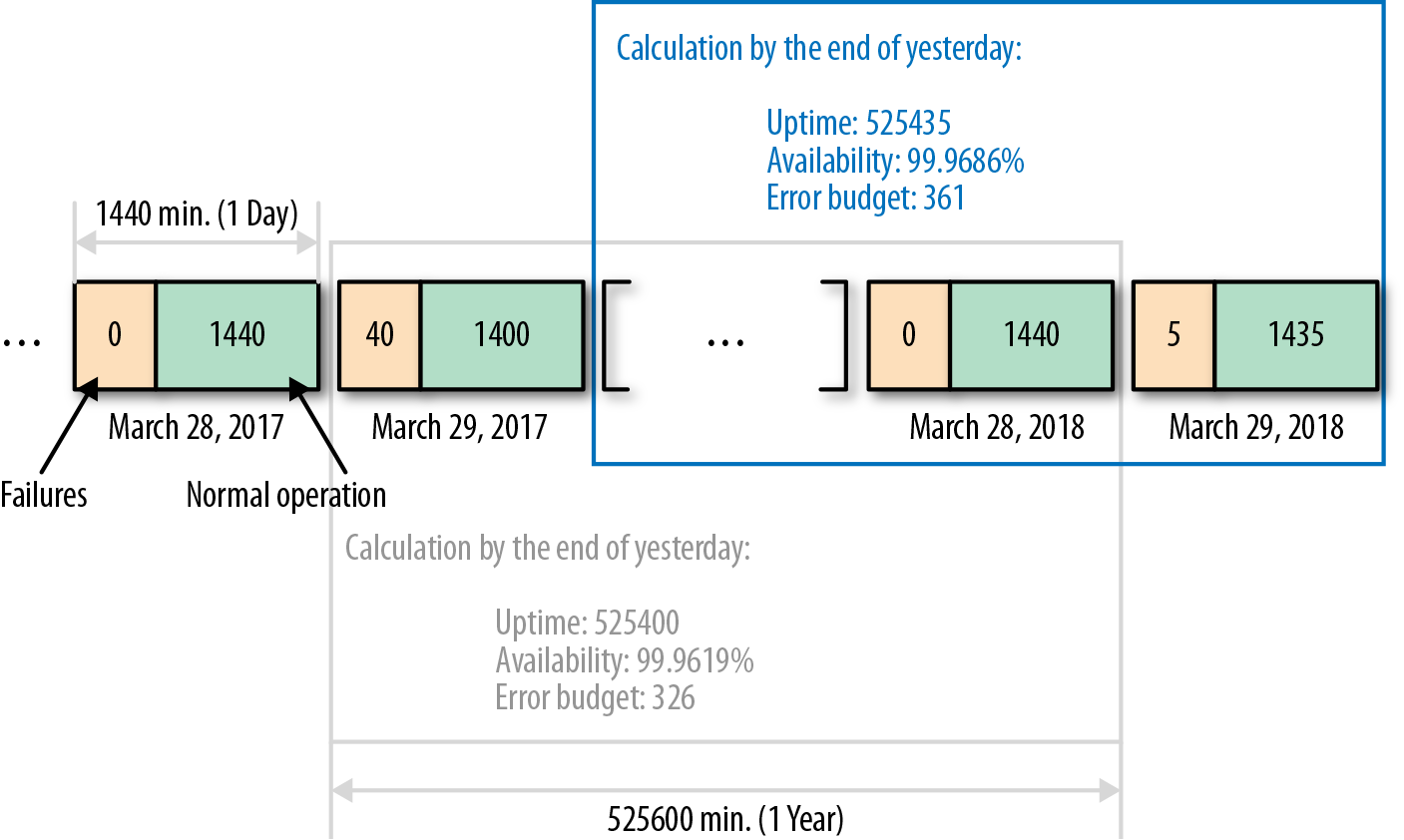
Figure 9-3. Daily availability calculation scope

Finally, the last thing we need to do is establish a way to convert our service’s failure counts into error budget amounts.

To avoid the previous problem in which a very few messages reflected on availability as a 33.33% drop, we will calculate day values, not as a single data set, but gradually by the smallest possible duration between available data points. For instance, if statistics are collected once a minute, we also can analyze the data on a per-minute basis.

The conversion itself is very simple. For every analyzed minute interval, we know the number of messages and the number of failures. One interval represents 100% of the time, and the total message amount is also treated as the 100% value. From this we can derive the failures fraction and extract the same amount from the time interval.

The sum of all converted failure times should be used to adjust current uptime and error budget values.

Let’s see how all that will work on the “Data receiver” example. For this component we have two types of failures:

• An error occurred, and we lost the message.

• The message is stuck somewhere for more than 10 ms.

We collect metrics on a per-minute basis, and we also produce all zero values (if there were no errors, we would produce a metric that explicitly says that “Errors=0.”). We also recalculate availability once every 24 hours.

For every minute interval, we have three data buckets:

• Number of messages processed

• Timers for every message

• Number of errors

If the timers bucket is missing a data point, we don’t know what exactly happened with that message and we mark it as a failure. Similarly, we do this with the number of processed messages and number of errors buckets, and if one of them is empty, we mark the entire minute as a failure.

Let’s recalculate our original example with 2 hosts and 10 messages and imagine that incident happened across a minute border and that was the only 10 messages for the entire 24-hour period. Here’s the calculation:

Minute 1

• Messages: 10

• Delays: 0

• Errors: 5

Minute 2

• Messages: 5

• Delays: 0

• Errors: 0

The uptime for the first minute is 0.5 minutes (50%), and 1 minute (100%) for the second minute. Overall, it is 0.5 minutes of downtime. Overall daily availability would be 1,439.5 minutes (1,440 – 0.5 = 1,439.5). In a worst-case scenario, if this incident were to spread over a longer time period and all messages happened to be delayed, we will lose only 20 minutes⁶ of a budget, which is quite different from the 33.33% we saw earlier.

Do not be surprised if a freshly established error budget drains out very quickly even from tiny incidents and the real availability level is much lower than you thought initially. We were establishing the SLA primarily to reveal this difference.

At this point, we are able to derive failures from other events; we know that they are not errors only. Also, we can convert these failures into the SLA-related values to track changes in the services’ availability level. And finally, we know how to calculate and use the error budget to plan time for experiments and to perform maintenance procedures without putting at risk agreements with our customers.

Now, let’s see what else we should keep in mind while working with SLAs.

Dealing with Corner Cases

To avoid the impression that involving SRE and establishing SLAs is a simple and straightforward way to address various difficulties and is only beneficial, here is a brief overview of a couple of notable corner cases when SLA by itself introduces a bit of additional complexity.

An SLA is not a constant, and to bring significant benefits, it should be well maintained and sometimes needs to be changed. On the other hand, the SLA should not be violated (by design). Moreover, not all projects need to have a strict SLA or involve SRE to maintain it.

An SLA is an agreement not only with the user, but also among developers, SREs, and management that are all committed to supporting this availability level. This means that “the level, as it is set, is the one that is needed.” An SLA violation is a severe incident, and to avoid it they all will need to interrupt their regular duties and put as much effort as needed to get the service back on track.

Not all agreements-related difficulties are introduced by errors and outages. Some of them are accumulated over the time span little by little. For example, take a case in which for the preceding six months the response latency gradually doubled and drew very close to the SLA limit. There might not be a single commit to the code that was responsible for that regression, but thousands of small modifications, each of which introduced its own few nanoseconds’ delay, can eventually double the original value. There would be no single developer or a team responsible for that. However, it is clear that we cannot leave this situation in place.

There are only two ways to deal with the situation at that point: adjust expectations (i.e., the list of indicators included into the SLA or the values that are related to one or several of these SLIs), or get under the hood and optimize the service.

For the first way, if it somehow turns out that the problem is not severe enough to pay additional attention to it, it means that we set our SLA incorrectly and need to make corrections. This case is the most typical for startup companies. Many small organizations have a certain period of growth when releasing new features is much more important than any other metric. The number of users at that time is very small, and minor inconveniences will be forgiven in favor of new functionality. If this describes your circumstances, the recommendation will be to downgrade your SLA to the status of an SLO and return to strict requirements later when the company gains a critical mass of customers. Another possibility is that we overestimated customer needs or, even more surprisingly, there might be an aspect of a service’s behavior that we previously treated as a minor one that over time became an exciting feature and a crucial part of the service.

For the second way, we need to deal with the issue from the technical perspective. The team should have a goal to return the problematic metric closer to its original state. To be clear, the goal is not to prevent latency growth caused by further product development; the goal is to reduce and keep the latency within a specified limit. We might introduce a bit of latency with a new feature, but at the same time it might be possible to decrease it again by refactoring an old component. Practically, we might dedicate one or two people to work on the optimization, while the rest of the team will continue working on ongoing projects. After a while (two weeks or a month), swap the people working on optimization with two other team members, similar to an on-call rotation.

Finally, it would be a mistake to say that every project needs to have an SRE onboard. Consider what would happen if we were involved with a project that does not require a high availability level. What if a maintained service was down for an entire weekend until developers brought it back online at the next business day and there was no negative impact at all? At the least, it would become a conflict of priorities because SREs and developers do not share the same availability goals and will drive the project in opposite directions. The number one priority for the developers might be to deliver new features as fast as they can, regardless of service availability, and the SREs will work hard to slow them down to, at least a little bit, stabilize the product. For such a project, having a SysAdmin who can help with system-level duties like initial configuration and supplementary software maintenance would be more than enough. So, before trying to apply SRE approaches to a particular service, we have to make sure that we do it in the right place. Otherwise, we will waste a lot of time and energy.

Conclusion

The SRE philosophy differs from that of the SysAdmin just by the point of view.⁷ The SRE philosophy was developed based on a simple, data-driven principle: look at the problem from the user and business perspectives, where the user perspective focuses on “take care of product quality,” the business perspective pays attention to “managing product cases and efficiency,” and “data-driven” signifies “not allowing assumptions.”⁸ Identify, measure, and compare all that is important. Everything else is the result of this. This is the core of all SRE practices.

If this all sounds very difficult and complicated, start with the following short list of instructions and summarized potential outcomes, applying it step by step to the smallest service component you have:

1. Begin a new project with the following quote: “Start with the customer and work backward.”

2. Divide large services into a set of components and treat each component as an individual service. That will help us to identify problematic spots easily.

3. List the vital service indicators (SLIs) that will provide us with a better understanding of what we should care about the most. Of course, we may not rely only on our beliefs and need to keep an eye on actual customers’ experience.

4. Indicators being aggregated to a complete SLO will explicitly express the meaning of a “good” and “bad” service state.

5. If the service you’re working with is already serving production traffic, try to pick values for the initial SLO such that they reflect the current service availability as close as possible. Work from that. This kind of SLO will not create an immediate necessity to change the service to match the desired level. We can raise the bar as the next step.

6. Start with a 100% uptime. Compute an error budget and make a list of all “failure” conditions that will reduce its size. It will help you track how much time is left for issues, maintenance, and experiments.

7. Enumerate all dependencies and their influence. This will be an important indicator of issue sources or performance regressions. You will need to consider whether an issue is caused by a problem with the service itself or due to a service with which it communicates.

8. Test service performance against SLO barrier values. That will indicate the relationship between traffic and required capacity.

9. During the test, measure not only how much incoming traffic the application is able to handle, but also how much additional load to external services it will generate. This will approximate the ratio between input and output (for every service separately), and precisely estimate requirements for dependent services. Repeat tests periodically, track changes in trends, and adjust capacity accordingly. Over time, an SLO will display the effective service reliability level, indicate regressions, and draw attention to problematic conditions.

10. Evaluate necessities and priorities for all technical and nontechnical decisions against the SLO and from a customer perspective.

11. Promote the SLO to SLA and establish a new objectives level; then move on to your next service.

Now, you can control your systems more accurately and can precisely know when, what, why, and how they should be adjusted. Following the “Focus on the user and all else will follow” principle, you can develop and enrich a set of your own best practices to gain efficiency, enjoy lower costs, and raise the bar for an overall positive customer experience.