
Chapter 19
Optimising RIAA realisation
(Linear Audio, Volume 7, Mar 2014)
This article is the sort of thing that happens when I sit on the sofa and let my mind wander. For no special reason, I began to think of the four different ways to make an RIAA network that were dealt with in Stanley Lipshitz’s famous paper [1]. An accurate RIAA network requires both precision resistors (which are relatively cheap) and precision capacitors (which are not). Given that it is hard to improve on the 5534 for noise performance with a Moving-Magnet (MM) cartridge, and it is not costly, it soon becomes clear that those precision capacitors will dominate the cost of an MM RIAA preamp stage. So the question was, for those four RIAA configurations, were there differences in how efficiently they used their capacitors? In other words, if all four were working at the same impedance, would some need more capacitance (and hence more money) to get the correct response? The answer was a resounding yes, my elation only slightly diminished by the realisation that I had been using the least efficient configuration for years. We live, and hopefully, learn.
Any accurate RIAA network will contain non-standard resistor and capacitor values. The resistors can be made up by using parallel pairs, and this not only gives a much more accurate nominal value than the nearest E24 resistor, but improves the accuracy of the combined value because random errors partially cancel. This is described in detail in the new edition of Small Signal Audio Design[2]. The capacitors are another story because the values available are usually much sparser than E24, often being E6.
For the resistors, I used these rules:
- The nominal value of the combination shall not differ from the desired value by more than half the component tolerance. For 1% parts, this means within ±0.5%.
- The resistors are to be as near-equal as possible, to get the maximum improvement possible over the tolerance of a single component. Thus two equal resistors, whether in series or in parallel, have the effective tolerance reduced by a factor of √2, while three have it reduced by √3, and so on.
- The E24 series of preferred values will be used.
The article reproduced here gives the subject a fairly thorough examination, and you may think the topic is pretty much exhausted. Not a bit of it. The examples given in the article use two resistors in parallel, and the relatively small number of combinations available means that the nominal value is not always as accurate as we would like; for example the 0.44% error in Table 19.3, which only just meets Rule 1 above.
This can be addressed by using three resistors in parallel. Given the cheapness of resistors, the economic penalties of using three rather than two to approach the desired value very closely are small, and the extra PCB area required is modest. However, the design process is significantly harder. Writing a bit of Javascript that explores all the feasible combinations of two-resistor in parallel is straightforward; you start with a resistor that is just above twice the target value, and put resistors from the E24 series in parallel until you have bracketed it with one result too high and the other too low. If neither answer is close enough to the target, increase the first resistor by one E24 step, then rinse and repeat. This process was used to generate all the resistor pairs in the article, and inevitably some are closer to the target than others. It does not look promising for dealing with three resistors because of the large number of combinations available.
To solve this problem, I made use of a table created by Gert Willmann, which he very kindly supplied to me. It lists all the three-resistor parallel combinations and their combined value. It covers only one decade but is naturally still a very long list, running to 30,600 entries. I applied it first to Figure 19.9 in the article. (+30dB gain, C1 set to exactly 33nF). The two-resistor values are shown in Table 19.3.
I started with R0, which has a desired value of 211.74Ω. The Willmann table was read into a text editor, and using the search function to find ‘211.74’ takes us straight to an entry at line 9763 for 211.74396741Ω, made up of 270Ω, 1100R, and 9100Ω in parallel. This is more than accurate enough—in fact it might be wise to increase the precision of the input value of 211.74Ω. However, since the resistor values are a long way from equal, there will be little improvement in accuracy; the effective tolerance calculates as 0.808%, which is not much improvement over 1%.
Looking up and down the Willman table by hand, so to speak, some better combinations were spotted that were more equal than others. For example. 390Ω 560Ω 2700Ω at line 9774 has a nominal value only 0.012% in error, while the tolerance is improved to 0.667%, and this is clearly a better answer. Scanning the table by eye is a bit of a tedious business, but it can be speeded up. The best result for improving the tolerance would be three equal resistors, but 620Ω 620Ω 620Ω has a nominal value 2.4 % too low, and 680Ω 680Ω 680Ω has a nominal value more than 7% too high, so obviously they are no good. But this does suggest that the first resistor should be either 560Ω or 620Ω, and armed with this clue searching by eye is faster. I found the best result for R0 is 560Ω 680Ω 680Ω at line 9754, which has a nominal value only −0.09% in error and an effective tolerance of 0.580%, which is very close to the best possible 0.577% (1/√3).
In contrast, the original two-resistor solution for R0 has a nominal value −0.33% in error and an effective tolerance of 0.718%.
Repeating the process for R1 (66.18kΩ desired) and searching for ‘661.8’ takes us to 1000Ω 2000Ω 91000Ω. Obviously with resistors outside the range 100Ω–999Ω, we need to scale by factors of 10; in this case by 100 times. This result has a very accurate nominal value but once more the tolerance is not brilliant at 0.74%. We need to cast our net wider. 660Ω x 3 is 1980Ω, so we look for 1800Ω as the first resistor, and we get 1800Ω 2000Ω 2200Ω. Scaling that up gives us 180kΩ 200kΩ 220kΩ. The nominal value is only 0.061% low, and the tolerance is 0.579%. It is hard to see how the latter value in particular could be much bettered.

Preface Figure 19.1
Part of the three-resistor Willmann table. This is the area around 211.7Ω
Repeating again for R2 (9432Ω desired), I got 22kΩ 33kΩ 33kΩ. The nominal value is only 0.036% low, and the tolerance is 0.589%.
The resistor R3 in the HF correction pole is less critical than the other components, as it only gives a minor tweak at the top of the audio band, but I applied the three-resistor process to it anyway. The desired value is 1089.3Ω. There are no suitable three-resistor combinations starting with 3000Ω, and the best I found was 2700Ω 2700Ω 5600Ω which has a nominal value error of −0.13% and a tolerance of 0.602%.
The final result is shown in Preface Table 19.1, which is Table 19.3 from the article rewritten with paralleled resistor triples; the errors in the nominal value column are now much smaller by factors between 12 and 1.2. It is an interesting question as to what the average improvement factor over a large number of two-resistor to three-resistor changes would be; I suspect (but am completely incapable of proving mathematically) that it’s going to be in the area of 3 to 4. The effective tolerances have been added as an extra column at the right, and you can see that all of them are quite close to the best possible value of 0.577% (1/√3). Preface Figure 19.2 shows the resulting schematic when Figure 19.9 in the article is redrawn with the new values. There is only one E24 resistor out of twelve, and all the others are E12. This is purely happenstance; no effort whatever was made to avoid E24 values. There is very little point in doing so unless you are using exotic parts that only exist as E12.
Preface Table 19.1 Table 19.3 in the article redone using paralleled resistor triples.
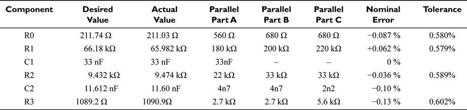

Preface Figure 19.2
The RIAA preamplifier in Preface Figure 19.9 of the article, with C1 = 33nF, redesigned with three parallel resistors to approach each non-standard value more closely, and have a smaller tolerance
I think it’s pretty clear that using three resistors instead of two gives much more accurate nominal values, and at the same time, a usefully smaller tolerance that almost halves the tolerance errors compared with a single resistor. Frequently, there are several suitable combinations, and you can choose between a more accurate nominal value or a smaller tolerance percentage.
The obvious question (to me, anyway) is: would four resistors be better? Not really. There is no point in having super-accurate nominal values if you are starting off with 1% parts. The tolerance is now halved, at best, but the improvement depends on the square-root of the number of resistors so we are heading into diminishing returns. If you want a better tolerance than three 1% resistors can give, the obvious step is to go to 0.1% resistors which are freely available, though they cost ten times as much as the 1% parts. Anything more accurate than that would be a specialised and very expensive item, and not obtainable from the usual component distributors.
I have applied the same process to the 3 × 10 nF design in Figure 19.12 of the article, and the result is shown in Preface Figure 19.3. There are now four E24 values out of twelve. The total value of C2 has been made more accurate (now −0.066%) by correcting the value of C2D; this has nothing to do with the three-resistor process.

Preface Figure 19.3
The RIAA preamplifier in Figure 19.12 of the article, with C1 = 3 × 10nF, redesigned with three parallel resistors
I also applied the process to the 4 × 10 nF design in Figure 19.14 of the article, and the result is shown in Preface Figure 19.4. There are now three E24 values out of twelve; I am starting to wonder if there is some mathematical property that means that E24 values are always in the minority. It seems unlikely, but if anyone with mathematical skills would like to tackle the question, the answer might be enlightening.

Preface Figure 19.4
The RIAA preamplifier in Figure 19.14 of the article, with C1 = 4 × 10nF, redesigned with three parallel resistors
Errata
This article is the only one which has not been reproduced here exactly as it was published, because unfortunately, a few numerical errors crept in that could cause confusion; they have been corrected here. My thanks to Gert Willmann for pointing these out. In the original article the errors were:
- In Figure 19.1 the correct value of T2 is 7950us, (not 7960us as in the original article) the correct value of f5 is 2122 Hz (not 2112 Hz as in the original), and the correct value of T6 is 1.35us (not 0.075us as in the original).
- In Table 19.4, the desired value for R1 should be 72.583kΩ, and the actual value 72.639kΩ. C2 should be 10.52nF instead of 11.60nF. The +0.34% error given in the final column is correct.
- In Figure 19.11, R1 should be 72.639kΩ.
- In Table 19.5 the error for R1 should be +0.19%. Also the desired value for R2 should be 7.782kΩ, as shown correctly in Figure 19.13; the actual value and the % error in Table 19.5 are also correct.
References
1. Lipshitz, S.P., On RIAA Equalisation Networks, J. Audio Eng Soc, June 1979, p. 458 onwards.
2. Self, D, Small-Signal Audio Design, 2nd edition, Chapter 2, pp. 48–56. Focal Press (Taylor & Francis) 2014. ISBN: 978-0-415-70974-3 Hardback. 978-0-415-70973-6 Paperback. 978-0-315-88537-7 ebook.
Optimising Riaa Realisation
RIAA equalisation is associated with moving-magnet (MM) pickups, but is no less necessary for moving-coil (MC) pickups. A very common arrangement is to have an MM input stage, with a suitable 47 kΩ input impedance, which can be switched between a directly-connected MM cartridge, and an MC cartridge followed by a flat low-noise gain stage. The noise conditions for the MM stage are very different in the two cases, but in either RIAA equalisation is required. This can be done in many ways, but some approaches can be discarded at once. Shunt-feedback RIAA stages for MM pickups are some 14 dB noisier than an equivalent series-feedback stage [1]; this is inherent because of the high inductance of MM cartridges, so we can lose that approach at once. Other methods split the various RIAA time-constant across separate stages, in various mixtures of passive and active circuits; this makes the calculations easy but uses more hardware and invariably involves compromises in headroom and noise performance.
If that sort of thing is the “brawn” hardware-heavy option, the “brains” option is to do all the RIAA equalisation in one stage, using series feedback. The “brains” part comes in because the interaction of the RIAA time-constants in a single feedback path makes the calculations for accurate RIAA much more difficult. Most of the hard work was done for us by Stanley Lipshitz, who in 1979 published comprehensive design equations for a large number of RIAA network configurations [2]. He deserves the thanks of us all. Nevertheless, these equations are pretty long and complicated, and adapting them to spreadsheet or MathCAD use is not a trivial business, so it is wise to assess which configurations are worth the effort before you undertake it.
At this point I am going to firmly state that the best way to implement RIAA equalisation is the conventional one-stage series-feedback method, using a gain of between +30 and +35 dB (at 1 kHz). Without going into all the detail of recorded levels and cartridge sensitivities, those gains will give more than adequate maximum input levels of 316 mVrms and 178 mVrms respectively. The output levels will be 158 and 281 mVrms respectively with a 5 mVrms input (1 kHz). The input stage will normally be followed by some form of controlled gain to get the signals up to the desired final level.
In this article RIAA accuracy is often worked out to a hundredth of a dB. That does not of course mean that such accuracy is essential for good listening, which is just as well as normal component tolerances would make it quite impossible. Instead the aim is to get the nominal results spot-on, so that whatever tolerances may do to us, we at least know we are aiming at the right values, and the practical results will be centred on them.
Equalisation and its discontents: The RIAA characteristic
The RIAA characteristic is probably the most complex standard equalisation curve in common use. Figure 19.1 shows the response asymptotes of its main features. The most important three corners in its response curve are f3 at 50.05 Hz, f4 at 500.5 Hz, and f5 at 2.122 kHz, which are set by three time-constants of 3180 μ sec, 318 μ sec, and 75 μsec. To put it concisely, the f3—f4 region allows for the constant-amplitude recording used over that range, while the plateau at f4—f5 allows for the high-frequency recording pre-emphasis which reduces noise by de-emphasis at playback.

Figure 19.1
The practical response for series-feedback RIAA equalisation, including the IEC Amendment which gives an extra roll-off at f2 (20.02 Hz).
In Figure 19.1 there is a further response corner at f2(20.02 Hz), corresponding to a time-constant of 7950 μs. This LF roll-off is called the “IEC Amendment” because it was added to the RIAA standard in 1976. It was intended to reduce the subsonic output, but its introduction is slightly mysterious. It was certainly not requested or wanted by either equipment manufacturers or their customers. Some manufacturers refused to implement it or just ignored it. It still attracts trenchant criticism today. The likeliest explanation for its introduction seems to be that various noise reduction systems (such as dbx), were then being promoted for use with vinyl and their operation was interfered with by subsonic disturbances (none of the systems caught on). In some preamps the IEC Amendment is switchable in/out.
The response in Figure 19.1 flattens out at f6, when the gain demanded by the RIAA network falls to unity, whereas to achieve the RIAA standard it ought to continue to drop at 6 dB/octave. This unwanted response corner is inherent in the series-feedback configuration, and is its only drawback. The gain in Figure 19.1 is +35 dB at 1 kHz, which puts f6 at 118 kHz, and this causes the gain to rise above the RIAA characteristic around 10–20 kHz; here it gives an excess gain of only 0.10 dB at 20 kHz, but the effect is more severe at lower gains because f6 occurs at lower frequencies. If the gain is reduced to +30 dB at 1 kHz to get more overload margin, the final zero f6 is now at only 66.4 kHz, introducing an excess gain at 20 kHz of 0.38 dB. This problem is completely cured by adding a lowpass time-constant after the stage; this is usually called an “HF correction pole” which means precisely the same thing. If the correct time-constant is used the gain and phase are corrected exactly.
The frequency f1 simply shows where the gain flat-tens out at the low-frequency end as once again it cannot fall below unity; it is usually of little or no importance.
A basic RIAA equalisation stage
Figure 19.2 shows a single-stage series-feedback MM preamp with a gain of +30 dB (1 kHz). It gives 158 mV out for 5 mV in (1 kHz), with an input overload level of 316 mV rms. This means an excellent overload margin of 36 dB, though more (variable) gain will be required later in most cases.
There are several different ways to arrange the resistors and capacitors in an RIAA network, all of which give identically exact equalisation when the correct component values are used. Of the four series RIAA configurations examined by Lipshitz, this is configuration A. It has the advantage that it is the simplest case when the Lipshitz equations are put into practice. Details that are essential for practical use, like input DC-blocking capacitors, DC drain resistors, and EMC/cartridge-loading capacitors have been omitted for clarity; in later diagrams the 47 kΩ input loading resistor is also omitted. The overall impedance of the RIAA network has been kept reasonably low by making R0 220 Ω; further reduction has virtually no effect on the noise performance and results in large and expensive RIAA capacitors. No attempt is made at this point to deal with the awkward values of R1 and R2. The notation R0, C0, R1, C1, R2, C2 is as used by Lipshitz; C1 is always the larger of the two.

Figure 19.2
Series-feedback RIAA equalisation in configuration A, designed for 30.0 dB gain (1 kHz) which allows a maximum input of 316 mV rms (1 kHz). The switchable IEC Amendment is implemented by C3, R3. HF correction pole R4, C4 is added to keep RIAA accuracy within ± 0.1 dB 20 Hz to 20 kHz.
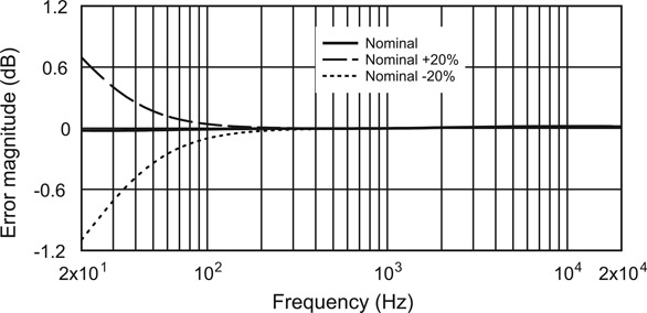
Figure 19.3
The effect of a ±20% tolerance for C0 when it is used to implement the IEC amendment in an amplifier; R0 = 220 Ω, gain +30 dB (1 kHz).
The unloved and unwanted IEC Amendment was no doubt intended to be implemented by restricting the value of C0; in this case the correct value of C0 would be 36.18 uF. This however leaves us wide open to significant errors due to the tolerance of an electrolytic capacitor. Figure 19.3 shows that the gain will be +0.7 dB up at 20 Hz for a +20% C0, and-1.1 dB down at 20 Hz for a-20% C0. The possible effect of C0 is less than ±0.1 dB above 100 Hz, but this is obviously not a great way to make dependably accurate RIAA networks. It also requires non-standard values for either R0 or C0.
Instead C0 is increased to 220 uF so that its-3 dB roll-off does not occur until 3.29 Hz. Even this wide frequency spacing introduces an unwanted 0.128 dB loss at 20 Hz (assuming no IEC amendment is used), and perfectionists will want to use 470 uF here, which reduces the error to 0.06 dB. The IEC amendment is now implemented passively after the amplifier stage, by non-electrolytic capacitor C3 (which can have a tolerance of ±1 %) in conjunction with R3, giving the required-3 dB roll-off at f2 (20.02 Hz). It is easier to make it switchable in/out. In Figure 19.2 we use a standard E3 capacitor value for C3; 470 nF was chosen, and as usual an unhelpful resistor value results; in this case R3 = 16.91 kΩ. Using E24 resistors, this can be implemented exactly as 16 kΩ + 910 Ω, though it has to be said near-equal series or parallel resistor pairs would give more accuracy for a given tolerance; more on that later. The switch as shown may not be entirely click-free because of the offset voltage at A1 output, but that is not important as it will probably only be operated a few times in the life of the preamp, if indeed ever.
We made C0 220 uF, which will be a handily compact component. Because it is not infinitely large there is, as we saw, an error of-0.128 dB at 20 Hz. It is possible to compensate for this by tweaking the IEC amendment frequency f2. If R3 is changed from 16.91 kΩ to 17.4 kΩ the overall response is made accurate to ±0.005 dB. The compensation is not mathematically exact- there is a + 0.005 dB hump around 20 Hz- but I suggest it is good enough for most of us. This process gets the nominal response right but does not of course do anything to reduce the effects of the tolerance of C0; these are however small, around + 0.05 dB.
Since the gain is +30 dB (1 kHz) f6 is at 66.4 kHz and an HF correction pole is essential. This is implemented by R4, C4 in Figure 19.2. There is no signifi-cant interaction with the IEC amendment, so we have complete freedom in choosing C4 and use a standard E3 value and then get the pole frequency exactly right by using two resistors in series for R4–470 Ω and 68 Ω. Since these components are only doing a little fine tuning at the top of the frequency range, the tolerance requirements are relaxed compared with the main RIAA network. The design considerations are a) that the resistive section R4 should be as low as possible in value to minimise Johnson noise, and on the other hand b) that the shunt capacitor C4 should not so large as to load the opamp output excessively at 20 kHz. It is assumed that an opamp such as the 5534 with good load-handling capability is used.
The IEC network is placed before the HF correction pole, as in Figure 19.2, so that R4 is not loaded by R3, which would cause a 0.3 dB loss, compromising noise or headroom slightly. As it is C3 is loaded by C4, but the loss is much smaller at 0.09 dB. It is assumed there is no significant external loading on the output at C4. Often the RIAA stage will be feeding the high-impedance input of a non-inverting gain stage, but if not buffering will be required so the two passive output networks behave as designed.
There is our basic RIAA stage. It works very well in both practice and theory, but is it the best solution possible? Here we set out on our voyage of optimisation.
Series-feedback RIAA-network configurations
Four possible configurations are described by Lipshitz in his classic paper.[2] These, using his component values, are shown in Figure 19.4; I have used the same identifying letters as Lipshitz. They are all accurate to within ±0.1 dB when implemented with a 5534 opamp, but in the case of configuration A the error is getting close to-0.1 dB at 20 Hz due to the relatively high closed-loop gain (+46.4 dB at 1 kHz) and the finite open-loop gain of the 5534. All have their RIAA networks at a relatively high impedance, and have relatively high gain and therefore a low maximum input. In each case the IEC amendment is implemented by the value of C0.
Burkhard Vogel in his weighty book The Sound of Silence describes configuration A as a Type-Eub network, configuration B a Fub-B network, and configu-ration C a Fub-A network [3]. He does not deal with configuration D.
Long ago I wrote a spreadsheet to implement the Lipshitz equations for configuration A simply because it was the easiest one to do. Repeating that for the remaining three configurations would be a fair amount of work, so the question arises, do any of the other three configurations have advantages over A that would make that work worthwhile?
Four things to examine suggested themselves:
- Each configuration in Figure 19.4 contains two capacitors, a large C1 and a small C2 that set the RIAA response. If they are close-tolerance (to get accurate RIAA) and non-polyester (to prevent capacitor distortion) then they will be expensive, so if there is a configuration that makes the large capacitor smaller, even if it is at the expense of making the small capacitor bigger, it is well worth pursuing. That large capacitor is almost certainly the most expensive component in the RIAA MM amplifier by a long way.
- I started by assuming that the signal voltages across each capacitor would be different. If polyester capacitors must be used for cost reasons, then if there is a configuration that puts less voltage across a capacitor then that capacitor will generate less distortion. Capacitor distortion at least triples, and may quadruple, as the voltage across it doubles, so choosing the configuration that minimises the voltage might be worthwhile. However, a good deal of simulation tells us that there is actually little difference between the four configurations as regards the magnitude of the signal voltage across the capacitors. Not a helpful result or an interesting result, but sometimes things just are that way.

Figure 19.4 The four RIAA feedback configurations in the Lipshitz paper.
- If we assume a certain amount of non-linearity in one or both of the RIAA capacitors, are the configurations different in their sensitivity to that non-linearity? In other words, how much distortion will appear at the output? This could be resolved in SPICE simulation, by using non-linear capacitor models constructed with Analog Behavioural Models, but it would be a lot of work, and since the emphasis of this article is on high quality, where we can presumably afford a polypropylene capacitor or two, I have put that one on the back-burner, though I hope it will not fall completely off the back of the cooker.
- My implementation of the Lipshitz equations starts off with the value of R0. Combined with the desired gain, it sets the impedance level of the whole RIAA network. A low impedance level reduces noise, but increases the size and cost of the precision capacitors C1 and C2. So just how low should R0 be for the best performance? This issue is examined at the end of this article.
That leaves us with 1) and 4), and in these cases we do get some useful results. Now read on …
The RIAA configurations compared for capacitor cost
We need to put the four configurations A, B, C, and D into a common form where they can be directly compared. In Figure 19.4 they are working at different impedance levels, as shown by the differing values of R0, and at different gains. To make the impedance levels the same we scale all the RIAA component values to make R0 exactly 200 Ω, as in Figure 19.5. C0 is then39.75 uF in each case, and implements the IEC amendment. The impedance scaling does not affect the gain or the RIAA accuracy; this was checked by simulation for each configuration. The new values for C1 and C2 are shown in Table 19.1.
Since the gains of configurations A, B, and C are nearly the same, we can roughly compare the values for C1, and it’s already starting to look as if A might in fact be the worst case for capacitor size. To be quite sure about this we can alter the gain of A to be exactly the same as B and C at +45.5 dB, which is easy as we already have the spreadsheet for it. We don’t have the tool for D. Configuration D has significantly bigger capacitors than A, B, and C because it has about half the gain but the same value of R0.

Figure 19.5
The four RIAA feedback configurations, with component values scaled so that R0 = 200 Ω in each case.
Table 19.1 The values of C1 and C2 in Figure 19.5, with networks scaled so R0 = 200 Ω in each case.
| Configuration | Gain at 1 kHz | Large cap C1 | Small cap C2 | C1/C2 ratio |
|
|
||||
| A | +46.4 dB | 8.235 nF | 2.298 nF | 3.583 |
| B | +45.5 dB | 7.794 nF | 2.685 nF | 2.903 |
| C | +45.5 dB | 5.841 nF | 2.012 nF | 2.903 |
| D | +40.6 dB | 13.38 nF | 3.528 nF | 3.791 |
We can change the gain of D by simply by scaling the RIAA network, with R0 kept constant. This will not be very accurate but should be good enough for us to compare the configurations. We have to increase the gain of D by 4.948 dB, or 1.767 times, so we divide capacitors C1 and C2 by this factor, and multiply resistors R1 and R2 by it. This gives the values shown in Figure 19.6 and Table 19.2. The C1/C2 ratios are naturally unchanged.
After this gain alteration, configuration D is definitely less accurate than before, but is still almost within a ±0.1 dB error band, only exceeding this (and not by much) over small frequency ranges. This is good enough to allow proper assessment of each configuration.
From Figure 19.6 and Table 19.2, we can see that C1 in configuration C is only 63% the size of C1 in configuration A. I expected this, but was afraid it might be accompanied by an increase in C2 in configuration C, but this is also smaller at 78% of C2 in A. I have to ruefully admit that configuration A (which I have been using for years) makes the least efficient use of its capacitors, since they are essentially in series, reducing the effective value of both of them. Configurations B and D have intermediate values for C1, but of these two D has a significantly smaller C2.
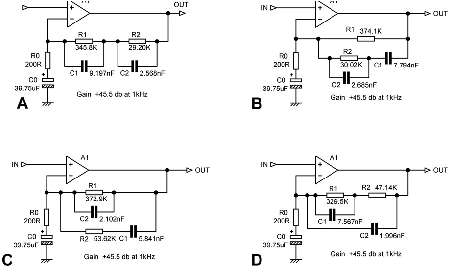
Figure 19.6
The RIAA feedback configurations, with component values scaled so that R0 = 200 Ω and the gain is +45.5 dB at 1 kHz in each case. Note that the RIAA response of D is here not completely accurate. The high gain means that the maximum input in each case is only 53 mV rms (1 kHz) which is not in general adequate.
Table 19.2 The values of C1 and C2 in Figure 19.6, after scaling so R0 = 200 Ω and gain =+45.5 dB (1 kHz) for all four configurations
| Configuration | Gain at 1 kHz | Large cap C1 | Small cap C2 | C1/C2 ratio |
|
|
||||
| A | +45.5 dB | 9.197nF | 2.568 nF | 3.581 |
| B | +45.5 dB | 7.794 nF | 2.685 nF | 2.903 |
| C | +45.5 dB | 5.841 nF | 2.012 nF | 2.903 |
| D | +45.5 dB | 7.567 nF | 1.996 nF | 3.791 |
Therefore configuration C would appear to be the optimal solution in terms of capacitor size, and hence cost and PCB area used. B and D appear to have no special advantages. It was now time to put together a software tool for the Lipshitz equations of C, so it could be designed accurately for gains other than +45.5 dB (1 kHz). As anticipated it was somewhat more difficult than it had been for configuration A, but no big deal.
We have already noted that a gain as high as +45.5 dB (1 kHz) gives an unacceptably poor overload margin. It has only used here so far because it was the gain adopted in the Lipshitz paper. If we assume an opamp can provide 10 Vrms out, then the maximum input at 1 kHz is only 53 mV rms. The gain of an MM input stage should not, in my opinion, much exceed 30 dB (1 kHz) See the earlier example in Figure 19.2.
My Precision Preamplifier design [4] has an MM stage gain of +29 dB (1 kHz), permitting a maximum input of 354 mV rms (1 kHz). The more recent Elektor Preamplifier 2012 [5] has an MM stage gain of +30 dB (1 kHz), allowing a maximum input of 316 mV rms; it is followed by a flat switched-gain stage which allows for the large range in MC cartridge sensitivity. Both designs use configuration A.
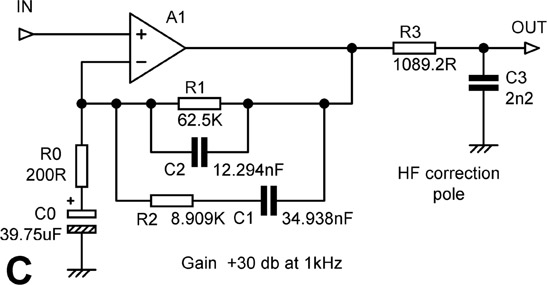
Figure 19.7
Configuration C with values calculated from the Lipshitz equations to give +30.0 dB gain at 1 kHz, and an accurate RIAA response within ±0.01 dB; the lower gain now requires HF correction pole R3, C3 to maintain accuracy at the top of the audio band.
A preamp with a gain of exactly +30 dB (1 kHz) using configuration C was therefore designed with the new software tool, and there it is in Figure 19.7. It has an RIAA response, including the IEC amendment that is accurate to within ±0.01 dB from 20 Hz to 20 kHz (assuming C0 is exactly correct in value). The relatively low gain means that an HF correction pole is required to maintain accuracy at the top of the audio band, and this is implemented by R3 and C3. If it was omitted the response would be 0.1 dB high at 10 kHz, and 0.37 dB high at 20 kHz. We use the E6 value of 2n2 for capacitor C3, so R3 is a non-preferred value.
In Figure 19.7, and in the examples that follow, I have implemented the IEC amendment by using the appropriate value for C0, rather than by adding an extra time-constant after the amplifier as in Figure 19.2. We have already seen that using C0 to do this is not the best method, but I have stuck with it here as it is instructive how the correct value of C0 changes as other alterations are made to the RIAA network.
Making C1 a single E6 capacitor
So far we have optimised our RIAA network by switching to configuration C. A further stage of refinement is possible after minimising C1 and C2. There’s nothing special about the value of R0 at 200 Ω (apart from the bare fact that it’s an E24 value), it just needs to be suitably low for a good noise performance. We can therefore scale the RIAA components again, not to make R0 a specific value, but to make at least one of the capacitors a preferred value, the larger one being the obvious candidate. Compared with the possible savings on expensive capacitors here, the cost of making up a non-preferred value for R0 is negligible.
In Figure 19.7, C1, at 34.9 nF, is suggestively close to 33nF. If we twiddle the new software tool for configuration C so that C1 is exactly 33 nF, we get the circuit in Figure 19.8. R0 has only increased by 6% to 212 Ω, and so the effect on noise performance will be negligible; I calculate it as 0.02 dB worse (with MM cartridge input load). All the other values in the RIAA feedback network have likewise altered by about 6%, including C0, but the HF correction pole is unchanged; that would only need to be altered if we altered the gain of the stage. Like Figure 19.7, the RIAA accuracy of this circuit is well within ±0.01 dB from 20 Hz to 20 kHz when a 5534 is used.
The circuit of Figure 19.8 now has two preferred-value capacitors, C1 and C3, but that is the best we can do. All the other values are, as expected, thoroughly awkward. In my book Active Crossover Design [6] I describe how to make up arbitrary resistor values by paralleling two or more resistors, and how the tolerance errors partly cancel. This also applies to capacitors. The optimal way to do this is with components of as near-equal values as you can manage. If the values are exactly equal, the combined accuracy is √2 time better than the individual components; the further away from equality, the less the improvement. Nothing more esoteric than the E24 series is assumed for the resistors. The optimal parallel pairs were selected in a jiffy using a specially written software tool. The parallel combination for C2, using E6 values, was done by manual bodging, though as you can see in Table 19.3, we have been rather lucky with how the values work out, with three parallel capacitors getting us very close to the desired value. Figure 19.9 shows the resulting circuit.

Figure 19.8
configuration C from Figure 19.7 with Ro tweaked to make C1 exactly the E6 preferred value of 33.000 nF. Gain is still 30.0 dB at 1 kHz, and RIAA accuracy within ±0.01 dB. The HF correction pole R3, C3 is unchanged.

Figure 19.9
configuration C from Figure 19.8 with the resistors made up of optimal parallel pairs to closely approach the correct value. C2 is made up of three parts. Gain +30.05 dB at 1 kHz, RIAA accuracy is worsened but still within ±0.048 dB.
Table 19.3 Approximating the exact values of Figure 19.8 with paralleled components, giving Figure 19.9.
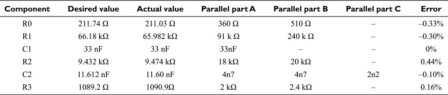

Figure 19.10
The RIAA accuracy of Figure 19.9. Gain is 30.05 dB at 1 kHz, and RIAA error reaches a maximum of +0.048 dB midband.
When selecting the parallel resistor pairs, the criterion I used was that the error in the nominal value should be less than half of the component tolerance, assumed to be ±1 %. R2 only just squeaks in at +0.44 %, but its near-equal values give almost all of the √2 improvement. Don’t forget that in Table 19.3 we are dealing with nominal values, and the % error in the nominal value shown in the rightmost column has nothing to do with the component tolerances.
Naturally the small errors in nominal value seen in the rightmost column of Table 19.3 have their effect. Figure 19.10 shows that the RIAA response now has a gentle peak of +0.048 dB at 1 kHz, which is by coincidence the worst-case frequency. Above that, the error slowly declines to +0.031 dB at 20 kHz. Most of this deviation is caused by the +0.44 % error in the nominal value of R2 (see Table 19.3).
C1 made up of multiple 10nF capacitors
We have just scaled the RIAA network so that the major capacitor C1 is a single preferred value; at 33nF it will probably be a rather expensive 1% polypropylene. RIAA optimisation can however be tackled in another way, depending on component availability. In many polysty-rene capacitor ranges 10 nF is the highest value that can be obtained with a tolerance of 1%. Paralleling several of these is a good deal more cost-effective than a single 1% polypropylene part. To exploit this we need to redesign the circuit of Figure 19.8 so that C1 is either exactly 30 nF or exactly 40 nF. Figure 19.11 shows the result for C1 = 30 nF. Ro has now increased to 233 Ω, which I calculate will degrade the noise by only 0.06 dB compared with R0 = 200 Ω (with MM cartridge input load).
The 40 nF version costs a bit more but gives a total capacitance that is twice as accurate as one capacitor (as √4 = 2), while the 30 nF version only improves accuracy by √3 (= 1.73) times. Figure 19.13 shows the result for C1 = 40 nF. R0 has now dropped to 175 Ω, which gives a calculated noise improvement of 0.04 dB. Not to belabour the point, but R0 has only a very minor effect on the noise-we will come back to that later. C0 is now larger at 45.51 uF.
Since in each case the gain is unchanged the values for the HF correction pole R3, C3 are also unchanged.
As for the previous example with C1 = 33nF, the awkward resistor values are made up with optimally-selected parallel pairs. The results of this process for C1 = 30nF are shown in Table 19.4 and Figure 19.12. In this case we have been unlucky with the value of C2, which needs to be trimmed with a 120 pF capacitor to meet the criterion that the error in the nominal value will not exceed half the component tolerance.
The same process can be applied to the 4 × 10 nF version in Figure 19.13, giving the component values in Table 19.5 and in Figure 19.14.
This time we are much luckier with the value of C2; three 4n7 capacitors in parallel give almost exactly the required value. On the other hand we are very unlucky with R0, where 180 Ω in parallel with 6.2 kΩ is the most “equal” solution falling within the error criterion.
Both my Precision Preamplifier ’96 [4] and the more recent Elektor Preamplifier 2012 [5] have MM stage gains close to +30 dB (1 kHz) like the examples above, but both use configuration A, and five paralleled 10 nF capacitors are required for C1. A third existing design using configuration A was modified to configuration C as in Figure 19.12, and thoroughly tested with an AP SYS-2702. The RIAA was exactly correct within the

Figure 19.11
Configuration C from Figure 19.8 redesigned so that C1 is now 30 nF, made up with three paralleled 10 nF capacitors. Gain +30.0 dB at 1 kHz, RIAA accuracy is within ±0.01 dB.

Figure 19.12
configuration C from Figure 19.11 with resistors made up of optimal parallel pairs, and C2 made up of four parts. Gain +30.0 dB at 1 kHz, RIAA accuracy is within ±0.01 dB.
Table 19.4 Approximation to the exact values in Figure 19.11 by using parallel components, giving Figure 19.12.

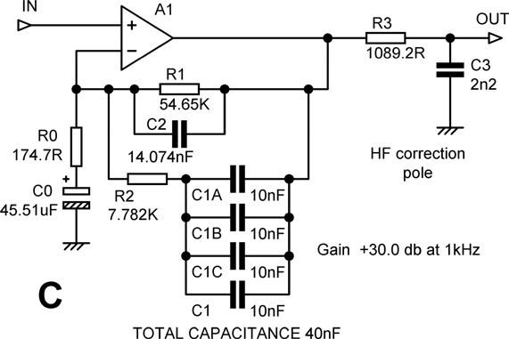
Figure 19.13
configuration C from Figure 19.8 redesigned so that C1 is 40 nF, made up with four paralleled 10 nF capacitors.
Gain +30.0 dB at 1 kHz, RIAA accuracy is within ±0.01 dB.
limits of measurement and the noise performance was unchanged. It gave a hefty parts-cost saving of some £2 on the product concerned.
Table 19.5 Approximation to the exact values in Figure 19.13 by using parallel components, giving Figure 19.14.

Noise & the value of R0
We have seen already that minor changes in the value of R0 have a negligible effect on the noise performance. The noise calculations were performed with MAG-NOISE2, an upgraded version of my MAGNOISE tool. This gives results within 0.2 dB of measurements and I believe it trustworthy.
In my published designs, R0 has gone from 470 Ω in 1979 [7] to 330 Ω in 1983 [8] and then 220 Ω in 1996 [4] as part of a general drive towards low noise by low-impedance design. I considered 220 Ω about as low as could be achieved while using a reasonable number (five) of paralleled 10 nF polystyrene capacitors for C1.
In MAGNOISE2, any source of noise can be switched off so its contribution can be assessed. R0 produces noise in two ways; its own Johnson noise, and the voltage produced by the opamp current noise flowing through it. At these impedances, the latter is negligible. Table 19.6 shows the results for 30 dB gain (1 kHz) using a 5534AN opamp and cartridge parameters of R = 610 Ω, L = 470 mH, for the values of R0 used in the discussions above, plus some more. The noise results are shown to two decimal places simply so that the small changes are visible; in practice they will be swamped by variations in opamp noise. R0 has only a minor effect; most of the noise comes from the Johnson noise of the cartridge resistance and the 47 kΩ input load, the opamp voltage noise, and the opamp current noise at the non-inverting input.

Figure 19.14
configuration C from Figure 19.13 with resistors made up of optimal parallel pairs. C2 is made up of three parts.
Gain +30.0 dB at 1 kHz, RIAA accuracy is within ±0.01 dB.
The first thing we see is that with R0 at my usual value of 220 Ω, we are only 0.39 dB noisier than some impossible circuit in which R0 did not exist at all. That is not an audible difference, and suggests that if we can accept just a little more noise we would be able to increase the impedance of the RIAA network and further reduce the amount of expensive capacitance required.
Looking at configuration C in Figure 19.11, with R0 = 233 Ω, we can redesign it, using the new software tool, so that C1 = 2 × 10 nF. Running the numbers, we get R0 = 349 Ω, as in Table 19.7, which Table 19.6 shows will be noisier than Figure 19.11 by only 0.18 dB. In many cases this will be an acceptable cost/performance trade-off. If we were happy with a 1.0 dB noise increase, R0 can go as high as 611 Ω.
For comparison Table 19.7 also shows the component values for configuration A, with C1 constrained to be 20 nF. Because of its inefficient use of capacitance, this requires R0 to be a good deal higher at 552 Ω, and the noise penalty referred to R0 = 233 Ω is 0.50 dB rather than 0.19 dB. This is rather less acceptable and confirms that configuration C is the best. Table 19.7 was checked by simulation and the RIAA accuracy is within ±0.01 dB from 20 Hz to 20 kHz.
Let’s push this a little further and assume we want C1 to be a single 10 nF 1% capacitor for real economy. What is the noise penalty? The software tools give us Table 19.8 for configurations C & A, and the noise penalties are inevitably larger, though perhaps not by as much as you would expect for fairly radical changes in the impedance of the RIAA network. Table 19.8 was checked by simulation and the RIAA accuracy is within ±0.01 dB from 20 Hz to 20 kHz.
All the noise calculations above are for a preamplifier driven by an MM cartridge with the parameters given above. As we noted at the start, the MM RIAA stage may also be driven from an MC head-amp. The noise conditions for the opamp are quite different, as it is now fed from a very low impedance, probably dominated by a series resistor in series with the MC amp output to give stability against stray capacitances. My current MC head-amp design has an EIN of -141.5 dBu with a3.3 Ω input source resistance [5]. Its gain is +30 dB, so the noise at its output is -111.5 dBu. The series output resistor is 47 Ω and its Johnson noise at -135 dBu is negligible, and so is the effect of the RIAA stage input noise flowing in it. The noise at the output of the RIAA stage is then -85.7 dBu, which is considerably higher than any of the figures in Table 19.6. In this application the value of R0 is uncritical.
Table 19.6 Calculated noise output for different values of R0 (22–22 kHz bandwidth, with RIAA), unweighted.
| Value of R0 | Noise out | Noise ref R0 = 0 Ω | Where used |
|
|
|||
| 0 Ω | −92.90 dBu | 0.00 dB | |
| 100 Ω | −92.72 dBu | +0.18 dB | |
| 175 Ω | −92.59 dBu | +0.31 dB | Figure 19.13 |
| 200 Ω | −92.55 dBu | +0.35 dB | Figure 19.7 |
| 212 Ω | −92.53 dBu | +0.37 dB | Figure 19.8 |
| 220 Ω | −92.51 dBu | +0.39 dB | Ref[4] |
| 233 Ω | −92.49 dBu | +0.41 dB | Figure 19.11 |
| 330 Ω | −92.33 dBu | +0.57 dB | Ref[8] |
| 349 Ω | −92.30 dBu | +0.60 dB | Table 19.7 C |
| 470 Ω | −92.11 dBu | +0.79 dB | Ref[7] |
| 552 Ω | −91.99 dBu | +0.91 dB | Table 19.7 A |
| 611 Ω | −91.90 dBu | +1.00 dB | |
| 699 Ω | −91.77 dBu | +1.13 dB | Table 8 C |
| 1000 Ω | −91.36 dBu | +1.54 dB | |
| 1104 Ω | −91.22 dBu | +1.68 dB | Table 8 A |
| 2000 Ω | −90.20 dBu | +2.70 dB | |
| 2310 Ω | −89.90 dBu | +3.00 dB | |
Table 19.7 Calculated RIAA components with C1 constrained to be 20 nF. IEC amendment implemented by C0.

Table 19.8 Calculated RIAA components with C1 constrained to be 10 nF; IEC amendment implemented by C0.

Conclusions
Our investigations have shown that there are very real differences in how efficiently the various RIAA networks use their capacitors, and it looks clear that using configuration C rather than configuration A will cut the cost of the expensive capacitors C1 and C2 in an MM stage by 36% and 19% respectively, which I suggest is both a new result and well worth having. From there we went on to find that different constraints on capacitor availability lead to different optimal solutions for configuration C.
We have also demonstrated that accepting very small amounts of extra noise allows us to increase the impedance of the RIAA network substantially, further reducing the capacitance required and saving some more of our hard-earned money.
I hope you will forgive me for not making public the software tools mentioned in this article. They are part of my stock-in-trade as a consultant engineer, and I have invested significant time in their development.
References
1. Self, Douglas, “Small Signal Audio Design” Focal Press 2010, p171; ISBN 978-0-240-52177-0
2. Lipshitz, S P, “On RIAA Equalisation Networks” J. Audio Eng Soc, June 1979, p458 onwards.
3. Vogel, Burkhard, The Sound of Silence, Springer 2nd edition 2011, p523; ISBN 978-3-642-19773-d
4. Self, Douglas, “Precision Preamplifier 96” Electronics World July/August and September 1996
5. Self, Douglas, “Elektor Preamplifier 2012” Elektor April, May, June 2012
6. Self, Douglas, “Active Crossover Design” Focal Press, 2011, pp342–350, ISBN 978-0-240-81738-5
7. Self, Douglas, “High-Performance Preamplifier” Wireless World, Feb 1979, p40
8. Self, Douglas, “Precision Preamplifier” Wireless World, Oct 1983, p31