
Chapter 6
Detecting the Number of Clusters through Cluster Validation
6.1. Introduction
The general approach to the identification of the number of clusters by means of cluster validation is to evaluate the quality of each k-cluster solution provided by the clustering algorithm and to select the value of k that originates the optimum partition according to the quality criterion [HAL 00]. Over the past decades, many approaches to cluster validation have been proposed in parallel to the advances in clustering techniques. Some of the most popular approaches have been introduced in Chapter 1, namely, the Dunn index [DUN 74, BEL 98, HAV 08], the Krzanowski and Lai test [KRZ 85], the Davies Bouldin score [DAV 79, HAL 02b], the Hubert’s γ [HAL 02a], the silhouette width [ROU 87], or, more recently, the gap statistic [ROB 01] (see chapter 1 for further details). Many of these strategies attempt to minimize/maximize the intra/intercluster dispersion.
Unfortunately, the performance of validation techniques usually depends on the dataset or the cluster algorithm used for partitioning the data. In addition, the distance metrics applied before clustering has proven a relevant factor for the final cluster solution. It may also influence the cluster validity success in determining the optimum number of clusters. In a few cases, prior assumptions about the dataset can be made. This enables the choice of the best fitting clustering technique and distance model. However, unsupervised models are often applied to more complex, multi-dimensional datasets for which little or no prior assumptions can be made, as it occurs with user utterances in troubleshooting agents.
In this chapter, a validity combination strategy is introduced to predict the number of clusters in a dataset even though no prior assumptions can be made about the clustering technique or distance measure. Our approach to cluster validation is to perform multiple simulations on a dataset varying the distance and clustering technique as well as the number of clusters k. Then, the different partitions obtained from these simulations are evaluated in parallel by several cluster validation criteria, thereby, a validation diversity is achieved, which can be exploited to measure the agreement/consistency of the different scores at each value k. This combination strategy is based on the calculation of quantile statistics of the validation curves, as explained in the following sections.
The individual validation indexes as well as the combination strategy have been first evaluated in four datasets: two synthetic sets (mixtures of five and seven Gaussians), the NCI60 microarray dataset, and the Iris dataset. Finally, the combination approach has been also applied for detecting the number of classes in a corpus of speech utterances from the framework of automated troubleshooting agents.
6.2. Cluster validation methods
In the following, let C = {C1,…,Ck} denote a cluster partition composed of k clusters and N the total number of objects in a dataset. Some existing techniques for validating the cluster partition are the following.
6.2.1. Dunn index
The Dunn index aims to identify the optimal solution that consists of compact and well-separated clusters [DUN 74, BEL 98]. According to this criterion, the index minimizes the intracluster distances while maximizing the intercluster distances. The Dunn index is defined as follows:
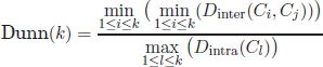
where the notations Dintra and Dinter stand for the intra- and intercluster distances, respectively. According to the Dunn objective, the optimum number of clusters corresponds to value k that maximizes Dunn(C).
6.2.2. Hartigan
This validation metric was proposed by Hartigan, the inventor of the k-means clustering [BAR 00] for detecting the optimum number of clusters k to apply in the k-means algorithm [HAR 75]:
where W(k) denotes the intracluster dispersion. The dispersion defined as the total sum of square distances of the objects to their cluster centroids. The γ parameter avoids an increasing monotony with increasing k. In this work, a small modification to the Hartigan metric has been introduced by treating the W(k) parameter as the average intracluster distance.
According to Hartigan, the optimum number of clusters is the smallest k that produces H(k)≤ η (typically η = 10). However, to allow a better alignment of the Hartigan index to other scores in the combination approach, a correction of the index has been applied in the form Hc(k)= H(k − 1). Thus, a modification of the optimum criterion has been accordingly applied by maximizing Hc(k). In other words, the new criterion maximizes the relative improvement at k with respect to k − 1, in terms of decreasing dispersion. This allows for a direct application of the corrected index Hc(k) in the combination approach without resorting to a previous inversion of the scores.
6.2.3. Davies Bouldin index
The Davies Bouldin index [DAV 79] was proposed to find compact and well-separated clusters. It is formulated as
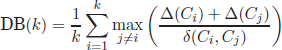
where Δ(Ci) denotes the intracluster distance, calculated as the average distance of all the Ci cluster objects to the cluster medoid, whereas the intercluster distance between two clusters δ(Ci,Cj) is the distance between the medoids of clusters Ci and Cj. The optimum number of clusters corresponds to the minimum value of DB(k).
6.2.4. Krzanowski and Lai index
This metric belongs to the so-called “elbow models” [KRZ 85]. These approaches plot a certain quality function over all possible values for k and detect the optimum as the point where the plotted curves reach an elbow, i.e. the value from which the curve considerably decreases or increases. The Krzanowski and Lai index is defined as
The parameter m represents the feature dimensionality of the input objects (number of attributes), and Wk is calculated as the within-group dispersion matrix of the clustered data
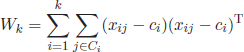
In this case, xij represents an object assigned to the ith cluster and ci denotes the centroid or medoid of the ith cluster. The optimum k corresponds to the maximum of KL(k).
6.2.5. Silhouette
This method is based on the silhouette width, an indicator for the quality of each object i [ROU 87]. The silhouette width is defined as
where a(i) denotes the average distance of the object i to all objects of the same cluster, and b(i) is the average distance of the object i to the objects of the closest cluster.
Based on object silhouettes, we may extend the silhouette scores to validate each individual cluster using the average of the cluster object silhouettes
Finally, the silhouette score that validates the whole partition of the data is obtained by averaging the cluster silhouette widths
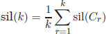
The optimum k is detected by maximizing sil(k).
6.2.6. Hubert’s γ
The Hubert’s γ statistic [HAL 02a, CHE 06] calculates the correlation of the distance matrix, D, to an a priori matrix, Y,
The γ statistic is formulated as
where N denotes the total number of objects in the dataset. The optimum number of clusters produces a maximum of the γ statistic.
6.2.7. Gap statistic
The idea behind the gap statistic is to compare the validation results of the given dataset to an appropriate reference dataset drawn from an a priori distribution, thereby, this formulation tries to avoid the increasing or decreasing monotony of other validation scores with increasing number of clusters.
First, the intracluster distance is averaged over the k clusters
where nr denotes the number of elements of the cluster r. The gap statistic is defined as
where E(log(Wk)) is the expected logarithm of the average intracluster distance. In practice, this expectation is computed through a Monte-Carlo simulation on a number of sample realizations of a uniform distribution B 1
where Wkb denotes the average intracluster distance of the 6th realization of the reference distribution using k clusters. The optimum number of clusters is the smallest value k such that Gap(k) ≥ Gap(k + 1) − sk+1, where ![]() is a factor that takes into account the standard deviation of the Monte-Carlo replicates (Wkb).
is a factor that takes into account the standard deviation of the Monte-Carlo replicates (Wkb).
6.3. Combination approach based on quantiles
As already introduced in section 6.1, a limitation of the validation indices is that their individual performances may vary significantly, depending on the dataset and/or clustering algorithm used for partitioning the data. According to [ROB 01] many validation indices are, to some extent, ad hoc approaches that were defined for specific problems, by assuming certain characteristics of a dataset or for their joint application with a given clustering algorithm. An example is the Hartigan index and the k-means clustering. Moreover, the clustering solution provided by the clustering algorithms may also depend on a particular distance function used to compute object dissimilarities. Therefore, the distance function is an additional factor that may influence the validation performance.
In this work, a combination approach has been implemented to achieve a robust solution. It does not require prior knowledge about the dataset nor the selection of a validation index, clustering method, or distance technique. The combination scheme aggregates multiple validation results obtained with the different validation indices, varying the clustering algorithm and distance functions. Any attempt to combine existing methods to increase the robustness of the solutions is in general known as the “knowledge reuse framework” [STR 02].
– Clustering techniques: In this work, four clustering algorithms have been used (from the R statistics package cluster) — the partitioning around medoids (PAM) algorithm [LEO 05] and the hierarchical complete, centroid, and average linkage methods [ALD 64,HAS 09,WAR 63].
– Distance functions: The aforementioned algorithms have been applied to two different distance matrices representing the dissimilarities between the dataset objects. To compute the distance matrices, two popular dissimilarity metrics have been selected — the Euclidean and cosine distances.
– Validity indices: Finally, some validity indices have been selected — the Hartigan, the Davies Bouldin, the Krzanowski and Lai test, the silhouete, and the gap statistic, which showed less strong monotony effects than the Dunn and Hubert´s γ indices in the analyzed datasets.
The different clusterings of the data obtained with the different clustering techniques and distance functions have been evaluated in parallel with the aforementioned validity indices2. This results in a diversity of validity outcomes, also referred to “validity curves.” In the following, let {![]() } denote the set of validity curves obtained from the previous validation experiments. Hence, each validity curve Vi indicates the validation scores obtained with each triple t (clustering algorithm, distance, and validity index), as a function of the number of clusters k. Note that Davies Bouldin scores have been inverted before applying the combination approach, so that the optimum can be generalized to the maximum scores and that the gap has been presented to the combination algorithm as
} denote the set of validity curves obtained from the previous validation experiments. Hence, each validity curve Vi indicates the validation scores obtained with each triple t (clustering algorithm, distance, and validity index), as a function of the number of clusters k. Note that Davies Bouldin scores have been inverted before applying the combination approach, so that the optimum can be generalized to the maximum scores and that the gap has been presented to the combination algorithm as
The proposed method has been motivated by the observation that, although individual validation curves may fail to determine of the optimum k, kopt, this value is located among the top scores in many cases. This fact suggested the combination of validation scores by means of p quantiles.
The p quantile of a random variable X is defined as value x which is only exceeded by a proportion 1 - p of the variable samples [SER 80,FRO 00]. In mathematical terms, if denoting the probability density function of the random variable X as pdf (X), the p quantile is defined as
Figure 6.1 illustrates this concept for an hypothetic random variable with a normal distribution of mean = 500.
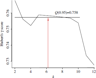
For the application of quantiles to the detection of the number of clusters, the different validation curves are treated as random variables. The quantile function is then applied to each single curve, Vi. The p quantile Q(Vi,p) equals the validation score ![]() only when exceeded by the 1 −p proportion of k values in the considered range. This is exemplified in Figure 6.2 for the validation curve obtained by applying the Hubert’s γ metric to a mixture of five Gaussians using the pair PAM-cosine.
only when exceeded by the 1 −p proportion of k values in the considered range. This is exemplified in Figure 6.2 for the validation curve obtained by applying the Hubert’s γ metric to a mixture of five Gaussians using the pair PAM-cosine.
Figure 6.1. Illustrative example of a p quantile: 0.5 and 0.9 quantiles of variable samples with normal distribution of mean = 500
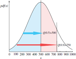
Figure 6.2. Application of quantiles to a validity curve (Hubert’s γindex, PAM clustering, and cosine distance on a mixture of five Gaussians). “Top scores” can be identified as such scores that exceed the p quantile level. In this example, p = 0.90
A basic approach to measuring the consensus of validity scores could be achieved by directly applying p quantiles to the set of validation curves and counting the number of times that each k value outperforms the score Q(Vi, p). This method has been called quantile validation (Qvalid(V, p)).
However, the Qvalid results show a certain dependency with the quantile probability parameter p. For example, using low p values often leads to maximum scores at the optimum kopt. However, maximum scores are also observed at undesired k, since there is a high proportion of samples that usually trespass the levels Q(Vi, p) for low p. In contrast, if a high p value is selected, a maximum peak can be clearly discerned. However, this maximum might be misplaced at k ≠ kopt. This happens, in particular, if an increasing/decreasing monotony with k is observed in some validity outcomes. These monotony effects may be captured in the Qvalid result in the form of maximum peaks misplaced at low/high k. 3
For these reasons a “supra-consensus” function has been proposed, called quantile detection, which aims to combine a set of quantile validation results obtained with different p values. Two alternatives have been analyzed to this aim: the first algorithm, QdetectA, is performed in two steps: first, the Qvalid algorithm (Qvalid(V,p)) is called with different p values: p = [0.1,0.2,...,0.9]. Then, the nine different Qvalid outputs are aggregated by counting the total number of (global or local) maxima placed at each k across these Qvalid outcomes.
The second alternative, QdetectB, is similar to the first algorithm except for a modification based on the scores given by Qvalid(V, p = 0.9). These scores are now placed with special emphasis with to reject potential spurious peaks in Qvalid scores for low p, which may yield false maxima in the aggregate solutions. In other words, the optimum number of clusters kopt should both lead to numerous maxima peaks of the Qvalid outcomes for any value p while still reaching a considerable Qvalid level for high p (p = 0.9).
6.4. Datasets
6.4.1. Mixtures of Gaussians
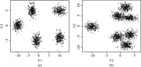
These synthetic datasets are mixture of five and seven Gaussians in two dimensions. The five Gaussian data comprise five well separable clusters without overlapping objects (Figure 6.3a). In turn, the seven Gaussian dataset contains a hierarchy of Gaussians with three well-differentiated groups and seven groups in which a high overlapping of objects can be observed. This second dataset was intended to evaluate how validation metrics behave on corpora with an underlying hierarchy of classes.
Figure 6.3. Mixture of Gaussian datasets. (a) Five Gaussians; and (b) seven Gaussians
6.4.2. Cancer DNA-microarray dataset
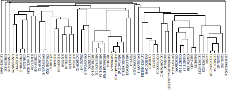
The NCI60 dataset [ROS 00] of the University of Standford has been also used (publicly available at [NCI 06]). It consists of gene expression data for 60 cell lines derived from different organs and tissues. The data are a 1, 375 × 60 matrix where each row represents a gene and each column a cell line related to a human tumor. A dendogram of the 60 clustered cell lines by using a complete-link hierarchical clustering algorithm can be observed in Figure 6.4. Nine known tumor types and one unknown can be distinguished. The cancer types associated with the labels of the dendogram leaves are as follows: LE, leukemia; CO, colon; BR, breast; PR, prostate; LC, lung; OV, ovarian; RE, renal; CNS, cns; ME, melanoma; and UN, unknown.
Figure 6.4. Example dendogram of DNA microarray data obtained by applying hierarchical complete-link clustering to the columns of the data matrix. Nine tumor types plus one unknown can be distinguished. The tumor types associated with the labels of the dendogram leaves are as follows: LE:leukemia; CO:colon; BR:breast; PR:prostate; LC:lung; OV:ovarian; RE:renal; CNS:cns; ME:melanoma; and UN:unknown
6.4.3. Iris dataset
The last dataset used in our validation experiments is the Iris dataset from the UCI machine learning repository. The dataset comprises 150 instances with four attributes related to three classes of Iris plants (Iris setosa, I. versicolor, and I. virginica). Two of the classes are linearly separable while one of them is not linearly separable from the other two.
6.5. Results
This section presents the validation scores obtained with the validity indices described in section 6.2 and our combination approach. Results obtained with the mixtures of Gaussians, NCI60, and Iris datasets are shown in Tables 6.1–6.4, respectively. The first rows show validation outcomes obtained with the validation indices (Hartigan, Dunn, Krzanowski and Lai, Hubert’s γ, Davies Bouldin, silhouette, and gap statistic) applied in combination with the PAM and average linkage clustering algorithms,4 using the cosine and Euclidean distances.
Finally, the second last row and the last row show validation scores obtained by the quantile detection approaches (QdetectA and QdetectB). It should be noted that, although the maximum k value used in our combination approach was k = 40, only an excerpt of the validation results for relevant k values close to the optimum is shown in Tables 6.1-6.4. Results outside this range have been omitted due to the limited space. Instead, significant results have been marked with asterisk symbols: (***) for first maxima (minima in the case of Davies Bouldin scores) versus (**) and (*) for second and third maxima, respectively. 5 Also, the columns corresponding to the correct number of clusters in each table have been highlighted in gray.
6.5.1. Validation results of the five Gaussian dataset
Results obtained with the mixture of five Gaussians can be observed in Table 6.1.
Most validation curves are able to identify the correct number of clusters (k= 5). In addition, the dependency of the validation scores with respect to the clustering conditions can be also observed. Some validation indices (Dunn, Krzanowski and Lai, Hubert, and gap statistic) are in some situations unable to detect the true number of clusters as a global maximum. These errors may be associated with the use of the cosine distance function, which, therefore, proves unsuitable for this dataset. However, the Krzanowski and Lai test and the gap statistic indices are still able to identify the optimum even with cosine distances.
Table 6.1. Validation results of the mixture of five Gaussian dataset The first 28 rows show some of the validation results obtained with the Hartigan, Krzanowski and Lai, Davies Bouldin, Dunn, Hubert’s , silhouette, and gap statistic indices. Next nine rows show the results of the Qvalid function for p = 0.1,0.2,...,0.9. Finally, the second last and last rows show the combined results obtained with the QdetectA and QdetectB algorithms.
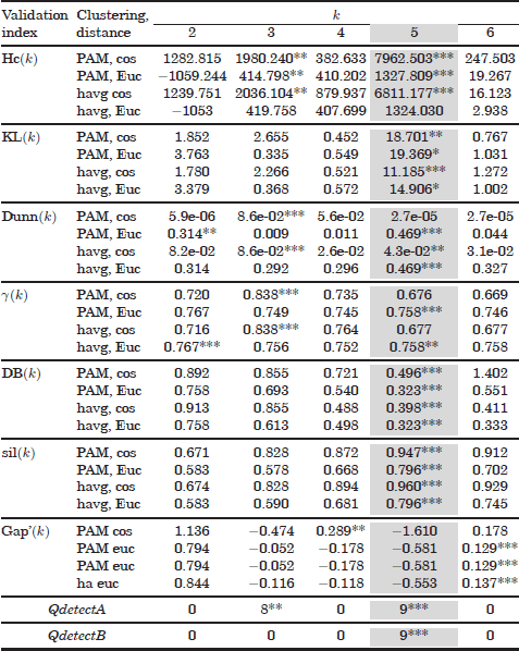
Table 6.2. Validation results of the mixture of seven Gaussians The first 28 rows show some of the validation results obtained with the Hartigan, Krzanowski and Lai, Davies Bouldin, Dunn, Hubert’s γ, silhouette, and gap statistic indices. For the Hartigan, KL, silhouette width, and gap statitics, the positions of global /local maxima in the range k = [2, 39] are indicated with asterisks. For the Davies Bouldin scores, asterisk symbols denote the position on global or local minima Finally, the second last and last rows show the combined results obtained with the QdetectA and QdetectB algorithms
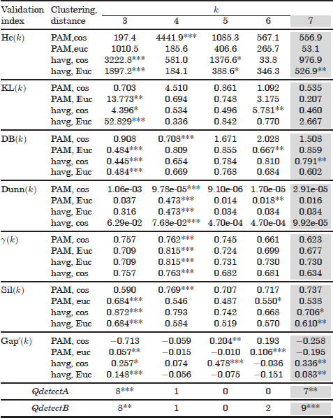
Table 6.3. Validation results of the NCI60 dataset
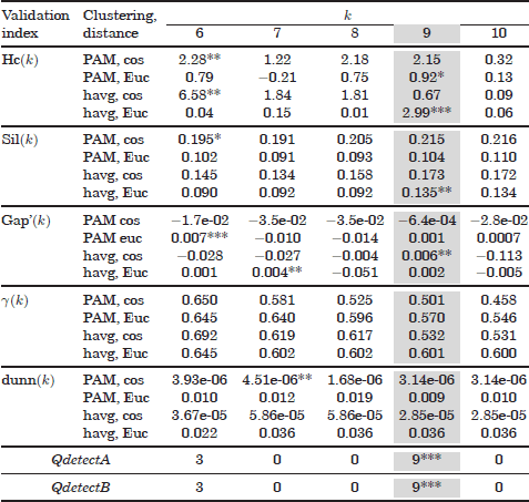
Table 6.4. Validation results of the Iris dataset
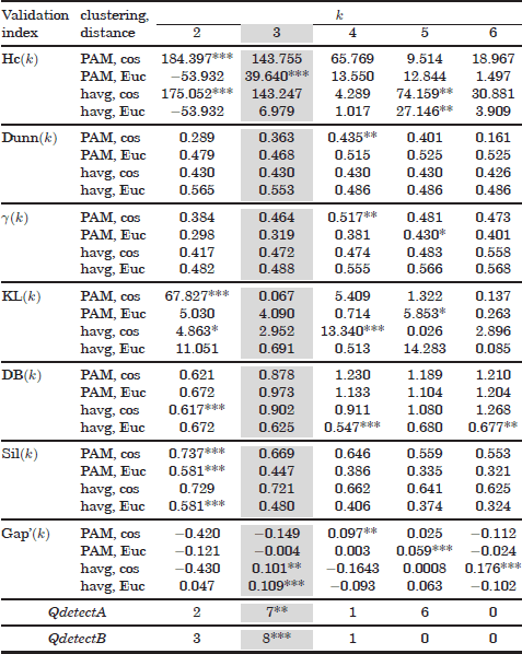
The QdetectA algorithm produces a global maximum at the true number of clusters. However, it should be noted that another global maximum peak is wrongly placed at k = 38. Finally, the second variant (QdetectB) places a unique maximum at k = 5 and is therefore able to discriminate the optimum number of clusters, kopt = 5.
6.5.2. Validation results of the mixture of seven Gaussians
The seven Gaussians mixture can be also observed as a hierarchy of three well separable groups and seven less separable clusters.
The high overlapping among classes in this dataset misleads the validity indices, as can be observed in Table 6.2. Some of the validity curves place the global maxima at k = 3, thus identifying the three bigger groups (upper hierarchy level). However, none of the analyzed curves has been able to place a global maximum at the true number of Gaussians (kopt = 7). Furthermore, only 5 validation curves of the 28 curves shown in Table 6.2 have achieved second local maxima at kopt.
Regarding the combination approach, the first proposed algorithm (QdetectA) also fails to detect the number of Gaussians as a global optimum. However, it is able to place a second local maximum at kopt, coinciding with the best validation curves. Finally, in contrast to the previous results, the QdetectB approach has correctly detected kopt as a global maximum.
6.5.3. Validation results of the NCI60 dataset
Table 6.3 shows some results obtained with the NCI cancer dataset. Note that validation curves obtained with the Davies Bouldin and Krzanowski and Lai metrics have not been included. This is due to the existence of missing values in the dataset, which yields missing values in the Davies Bouldin and Krzanowski and Lai functions used.
In this dataset, only the (corrected) Hartigan index is able to detect the number of classes in one of the validation curves. This occurs when hierarchical average clustering is used in combination with the Euclidean distance. Other three validation curves place local maxima at kopt = 9. Second local maxima are achieved at kopt by the silhouette and gap metrics with hierarchical average clustering, and a third local maximum is placed by the Hartigan in combination with the PAM algorithm and Euclidean distance.
Regarding our combination approach, both algorithms, QdetectA and QdetectB, have discovered the correct number of classes at kopt.
6.5.4. Validation results of the Iris dataset
Table 6.4 shows the validation results with the Iris dataset. This dataset is composed of two linearly separable Iris types and one third Iris class nonlinearly separable from the other two. Therefore, most validation curves fail to detect the number of clusters. Validation maxima are often misplaced at k = 2. Only the Hartigan and gap indices, in combination with the Euclidean distances and the PAM and hierarchical average algorithms, respectively, are able to identify the correct number of classes. Also, the gap statistic with the hierarchical average clustering and the cosine distance places a second maxima at k = 3.
These validation outcomes have been slightly improved by the QdetectB algorithm. Using this method, a second local maximum is placed at kopt = 3. The global maximum is found at k = 24, and other local maxima are located at k = 26 and 32. Finally, as with the previous datasets, the QdetectB variant is able to identify the true number of clusters in the Iris dataset.
6.5.5. Discussion
The mixture of seven Gaussians can be divided in a hierarchy of three well separable clusters and seven, less separable clusters (optimum). In this situation, the evaluated validation indices generate numerous errors: the three top clusters are frequently identified instead of the seven existing Gaussians. Only the Hartigan, silhouette, and gap statistic find some local maxima at the optimum. However, despite the numerous errors, the combination approach is still able to identify the seven Gaussians if using the QdetectB algorithm. The first alternative (Qdetect) places a second local maximum at kopt, coinciding with the best validation curves.
Validation errors can again be observed in individual validation curves on the NCI60 and Iris datasets, for which global and local maxima are barely placed at kopt = 9 and kopt = 3. In these datasets, combined results clearly outperform individual validation results. On the NCI60 dataset, both algorithms (QdetectA and QdetectB) place the global maxima at kopt = 9. On the Iris dataset, QdetectB achieves a global maximum at kopt = 3 versus a second local maximum obtained by QdetectA.
Furthermore, the observed results allow a comparative evaluation of validation indices. In general, the Hartigan, silhouette, and gap statistic indices have provided better performances than the Dunn, Hubert’s γ and KL indices, although their performances clearly depend on the clustering settings (clustering algorithm and distances).
To summarize, it can be concluded that the QdetectA algorithm performs equal or better than the best of the validity curves, in terms of the maximum peaks achieved at kopt, while the second variant, QdetectB, has been able to detect the optimum number of cluster on all analyzed datasets. In the next section, the performances of both validity combination approaches on a corpus of SLDS speech utterances are analyzed.
6.6. Application of speech utterances
The validation approaches to detect the number of clusters have been also applied to a corpus of speech utterances in the framework of automated troubleshooting agents.
As outlined in Chapter 1, a set of problem categories in a troubleshooting domain is currently defined by the dialog interaction designers. However, it is desirable to develop tools that aim to automatically redefine the set of problem categories with minimum human supervision. Such tools can enable a rapid adaptation of the systems and their portability to different domain data.
Therefore, two combination approaches (QdetectA and QdetectB) have also been applied for detecting the number of potential problems in a given troubleshooting domain, which provided a corpus of transcribed utterances related to this domain. In particular, the utterance corpus used in this work is related to the video troubleshooting domain and has been collected from user calls to commercial video troubleshooting agents. The corpus comprises 10,000 transcribed training utterances. Reference topic categories (symptoms), defined by the agent interaction designers, are also available. The number of reference topic categories is k = 79. Some examples of utterances and their associated reference categories are
– “Remote’s not working” (CABLE)
– “Internet was supposed to be scheduled at my home today” (APPOINTMENT)
– “I´m having Internet problems” (INTERNET)
6.7. Summary
In this chapter, different approaches for the discovery of the true number of clusters in a dataset have been analyzed. First, seven existent approaches in the literature to the optimum detection have been introduced: the Hartigan, Dunn, Hubert’s γ statistic, Davies Bouldin, gap, and silhouette width indices. The weakness of individual validity indices is related to the fact that the methods have been proposed for solving somewhat ad hoc problems or datasets and, therefore, their performance depends on the clustering algorithm, distance metric, or even on the dataset on which the validation indices are applied. This dependency has been evidenced through an analysis of the scores obtained by the different indices in synthetic and real datasets using four different clustering algorithms and two classical distance metrics (Euclidean and cosine).
Two approaches to the discovery of the number of clusters have been proposed to reduce the “ad hoc” performances of individual metrics. The main assumption was that, although the optimum could not be clearly visible in all individual metrics, the multiplicity of existing methods can be exploited to detect underlying “agreements” between the scores. In other words, the optimum (kopt) is hidden among the top scores in the validation curves and can be uncovered by adequately measuring the consensus between the different validation outcomes. The proposed approach is to measure this agreement by calculating p quantiles (points among the 1− p “top scores”). The quantile approach has proven highly adequate for discovering the hidden optimum in most datasets.
However, the optimum detection on the video troubleshooting agent has proven a task of high complexity, possibly due to the broad range of k values analyzed for the optimum search. The optimum (k = 79) could not be identified either by the validation curves or by the quantile approach due to a rapid variation of the obtained scores with k, as well as the strong monotony of the curves with k. The QdetectA produced six maxima at k = {6, 18, 72, 89, 102, 126}, while the QdetectB algorithm failed to detect the optimum due to an aggressive exclusion of k values using p = 0.9 quantiles.
In parallel to the number of clusters detected, our future steps are toward the identification of the best fitting clustering algorithm and distance model, given a fixed number of clusters. A similar approach to the one developed in this work based on p quantiles can be used for this aim, applied to the set of validation curves obtained with each pair (clustering technique and distance function) with the set of validity indices and comparing these scores with the “global” scores obtained for detecting the optimum number of clusters. Another alternative is the application of cluster ensembles to reach a good compromise solution between the different clustering algorithms [STR 02].
1. Note that the reference data drawn from this uniform distribution consists of a number, N, of objects identical to the dataset, with identical number of features m. The values of each feature in each object are assigned randomly in the original feature range.
2. Note: While Hartigan, Krzanowski and Lai, Davies, and silhouette have been used in combination with the four clustering algorithms, the gap statistic has been only applied with the PAM and average linkage algorithms.
3. Note that p quantiles for very high p values (e.g. p = 0.9) pose a strong condition to the validity curves: the captured k values for this high quantile often correspond to the global maximum peaks or k values in a close neighborhood. However, an important proportion of the validation curves may not be capable to place the (global) maximum peak at kopt, as motivated by the present work. Hence, the “agreement” measured by the Qvalid function for high p is considerably lower than the agreements achieved for low p. Owing to this low scores, if monotony effects are observed in some validation curves, it is possible that a “false agreement” is produced with a Qvalue, which can even exceed the Qvalid score at kopt.
4. Note that the resulting validation curves V have been obtained as a combination of the Pam and hierarchical average, single and centroid linkage methods. However, concerning individual validation curves, only results with the Pam and hierarchical linkage methods are shown in the tables for simplicity purposes.
5. A local maxima is considered at k if the score is higher than the values of k +1 and k−1. For edge values (k = 2, k = 40), a local maxima is considered if these scores are greater than their adjacent in-range neighbors’ scores.