
Chapter 5
Detection of the Number of Clusters through Non-Parametric Clustering Algorithms
5.1. Introduction
As described in Chapter 1, the identification of the optimum number of clusters in a dataset is one of the fundamental open problems in unsupervised learning. One solution to this problem is (implicitly) provided by the pole-based clustering (PoBOC) algorithm proposed by Guillaume Cleizou [CLE 04a]. Among the different clustering approaches described in Chapter 1, the PoBOC algorithm is the only method that does not require the specification of any kind of a priori information from the user. The algorithm is an overlapping, graph-based approach that iteratively identifies a set of initial cluster prototypes and builds the clusters around these objects based on their neighborhoods.
However, one limitation of the PoBOC algorithm is related to the global formulation of neighborhood applied to extract the final clusters. The neighborhood of one object is defined in terms of its average distance to all other objects in the dataset (see section 2.1). This global parameter may be suitable for discovering uniformly spread clusters on the data space. However, the algorithm may fail to identify all existing clusters if the input data are organized in a hierarchy of classes, in such a way that two or more subclasses are closer to each other than the average class distance.
To overcome this limitation, a new hierarchical strategy based on PoBOC has been developed called “hierarchical pole-based clustering” (HPoBC). The hierarchy of clusters and subclusters is detected using a recursive approach. First, the PoBOC algorithm is used to identify the clusters in the dataset, also referred to as “poles.” Next, under the hypothesis that more subclusters may exist inside any pole, PoBOC is again locally applied to each initial pole. A cluster validity based on silhouette widths is then used to validate or reject the subcluster hypothesis. If the subcluster hypothesis is rejected by the silhouette score, the candidate subclusters are discarded and the initial pole is directly attached to the final set of clusters. Otherwise, the hypothesis is validated and the new identified poles (subclusters) are stored, and a similar analysis is performed inside each one of these poles. This procedure is applied recursively until the silhouette rejects any further hypothesis. The HPoBC method is explained in more detail in the following sections and is compared with other traditional algorithms (hierarchical single, complete, average, and centroid linkages as well as the partitioning around medoids algorithms).
5.2. New hierarchical pole-based clustering algorithm
The new clustering method is a combination of the PoBOC algorithm and hierarchical divisive clustering strategies. In a divisive manner, the proposed hierarchical approach is initialized with the set of poles identified by PoBOC (see Chapter 1) and is recursively applied to each obtained pole, searching for possible subclusters.
5.2.1. Pole-based clustering basis module
To detect the set of poles in the hierarchical method HPoBC, the graph construction, pole construction, and pole restriction stages of POBOC have been preserved. However, the affectation step has been replaced by a new procedure called pole regrowth:
The pole-regrowth procedure is an alternative to the PoBOC single affectation for re-allocating overlapping objects into one of the restricted poles. As it can be observed in Figure 5.1(a), not only a pole but also an overlapping region may contain potential subclusters. If each overlapping object xi is individually assigned to the pole maximizing membership u(xi,![]() ), the objects inside a single cluster might be assigned to different poles. 1 The pole-regrowth procedure is intended to avoid any undesired partitioning of clusters existing in overlapping areas while re-allocating residual objects.
), the objects inside a single cluster might be assigned to different poles. 1 The pole-regrowth procedure is intended to avoid any undesired partitioning of clusters existing in overlapping areas while re-allocating residual objects.
Figure 5.1. Example of the pole growth. (a) Two restricted poles (red and green circles) and their overlapping objects (black circles) — from the database 1000p9c, see Figure 5.2(q). (b) New poles obtained after the re-allocation of the overlapping objects by the pole regrowth method
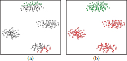
An example of the pole-regrowth method is shown in Figure 6.3. Figure 5.1(a) shows two restricted poles in red and green colors, respectively. All points between these restricted poles are overlapping points. It can be observed that many of these points build another two clusters, which PoBOC fails to detect. The re-allocation of overlapping points by the pole-regrowth procedure is illustrated in Figure 5.1(b). A single affectation would have split each overlapping cluster into two halves (upper and bottom). Using the pole-regrowth method, all objects inside each overlapping cluster have been jointly assigned to a single pole. This fact allows us to detect the overlapping clusters in further recursive steps.
We refer to the modified PoBOC algorithm as pole-based clustering module, which is the basis for the hierarchical approach described in the following paragraphs.
5.2.2. Hierarchical pole-based clustering
The new hierarchical version of PoBOC is called HPoBC.
First, the pole-based clustering module is applied to the entire dataset to obtain an initial set of poles. Then, a recursive function, the pole-based subcluster analysis, is triggered on each pole with more than one object. If an individual pole is found, the corresponding object is attached to the set of final clusters as an individual cluster. This recursive function is continuously called with the objects of each obtained pole, internally denoted ![]() , because it refers to an upper level in the hierarchy. Analogously, the new set of poles found on
, because it refers to an upper level in the hierarchy. Analogously, the new set of poles found on ![]() is denoted
is denoted ![]() , indicating a lower hierarchy level. These poles represent candidate subclusters. To decide whether
, indicating a lower hierarchy level. These poles represent candidate subclusters. To decide whether ![]() compounds are “true” subclusters or not, a criterion typically used for cluster validity is applied, namely, the average silhouette width, described in Chapter 1 [ROU 87]. The average silhouette width of a cluster partition returns a quality score in the range [—1,1], where 1 corresponds to a perfect clustering. According to [TRE 05], a silhouette score smaller or equal to sil = 0.25 is an indicator for wrong cluster solutions. However, from our experiments, a more rigorous threshold sil > 0.5 has proven adequate for validating the candidate subclusters. 2 The problem of deciding whether a dataset contains a cluster structure or not is commonly referred to as cluster tendency in the cluster literature [JOL 89]. If the quality criterion is not fulfilled (sil < 0.5) the subcluster hypothesis is rejected, and the top cluster
compounds are “true” subclusters or not, a criterion typically used for cluster validity is applied, namely, the average silhouette width, described in Chapter 1 [ROU 87]. The average silhouette width of a cluster partition returns a quality score in the range [—1,1], where 1 corresponds to a perfect clustering. According to [TRE 05], a silhouette score smaller or equal to sil = 0.25 is an indicator for wrong cluster solutions. However, from our experiments, a more rigorous threshold sil > 0.5 has proven adequate for validating the candidate subclusters. 2 The problem of deciding whether a dataset contains a cluster structure or not is commonly referred to as cluster tendency in the cluster literature [JOL 89]. If the quality criterion is not fulfilled (sil < 0.5) the subcluster hypothesis is rejected, and the top cluster ![]() is attached to the final clusters. Otherwise, we continue exploring each subcluster to search for more possible sublevels.
is attached to the final clusters. Otherwise, we continue exploring each subcluster to search for more possible sublevels.
5.3. Evaluation
The PoBOC algorithm as well as the HPoBC algorithm has been compared with other hierarchical approaches:
the single, complete, centroid, and average linkage and the divisive analysis (DiANA) algorithm. These classical algorithms are examples of clustering approaches that require the target number of clusters (k) to find the cluster solutions. To enable a comparison of PoBOC and HPoBC to the hierarchical agglomerative and divisive approaches, these algorithms have been called with different values of the k-parameter. Thus, the average silhouette width has been applied to validate each solution and predict the optimum number of clusters, kopt. It should be noted that, in the HPoBC algorithm, the average silhouette width has also been applied with a different purpose. Instead of using the silhouette width as a (global) validation index, it has been applied in a recursive and local manner to evaluate the cluster tendency inside each obtained pole.
5.3.1. Cluster evaluation metrics
For a comprehensive evaluation of the discussed algorithms, their cluster solutions have also been compared with the reference category labels, available for evaluation purposes, using three typical external cluster validation methods: entropy, purity, and normalized mutual information (NMI) (see Chapter 2).
5.4. Datasets
The described approaches have been applied to the synthetic datasets of Figure 5.2. The first dataset (100p5c) comprises 100 objects in 5 spatial clusters (Figure 5.2(a)), the second dataset (6 Gauss) is a mixture of six Gaussians (1500 points) in two dimensions (Figure 5.2(e)). The third dataset (3 Gauss) is a mixture of three Gaussians (800 points) in which the distance of the biggest class to the other two is larger than the distance among the two smaller Gaussians (Figure 5.2(i)). This dataset illustrates a typical example in which using cluster validity based on Silhouettes may fail to predict the number of classes due to the different interclass distances. The fourth and fifth data (560p8c and 1000p9c) contain 560 and 1000 points in two dimensions, with 8 and 9 spatial clusters, respectively (Figure 5.2(m) and (q)).
The cluster solutions provided by the PoBOC, the HPoBC, and an example hierarchical agglomerative approach (average linkage) are shown in the plots of Figure 5.2 (different colors are used to indicate different clusters).
5.4.1. Results
As can be seen in Tables 5.1–5.5, the performance of the HPoBC algorithm is consistently superior to the original PoBOC algorithm on all datasets and metrics. The classical (divisive and agglomerative) approaches with the help of silhouettes to determine the optimum k are also able to detect the class structure in three datasets (100p5c, 1000p9c, and 6 Gauss). The performance of classical approaches is thus comparable to the HPoBC algorithm on the explained datasets. Note that, in some cases, the NMI score achieved by the HPoBC is marginally lower (≤ 1.8%) than other hierarchical approaches, due to the false discovery by the HPoBC of tiny clusters in the boundaries of a larger cluster. In contrast to the previous datasets, the DiANA and agglomerative hierarchical approaches fail to capture accurately the existing classes on the datasets 560p8c and 3 Gauss. The problem lies in the silhouette scores, which fail to place the maximum (kopt) at the correct number of clusters. This happens because the intraclass separation differs significantly among the clusters. However, this problem is not observed in the HPoBC algorithm, since silhouette scores are used to evaluate the local cluster tendency. This implies a more “relaxed” condition in comparison to the use of silhouettes for validating global clustering solutions. Thus, in these cases, the HPoBC algorithm is advantageous with respect to the classical hierarchical approaches, as evidenced by absolute NMI improvements around 10%.
Figure 5.2. Spatial databases and the extracted clusters using PoBOC, HPoBC, and the average linkage clustering algorithms. (a) Dataset with 100 points in 5 spatial clusters (100p5c), (e) mixture of six Gaussians, 1500 points (6 Gauss), (i) mixture of three Gaussians (3 Gauss), (m) 560 points, 8 clusters (560p8c), and (q) 1000 points, 9 clusters (1000p9c). (b), (f), (j), (n), and (r) Poles detected by PoBOC in the datasets. (c), (g), (k), (o), and (t) Clusters detected by the new HPoBC algorithm (black circles indicate patterns detected as outliers by the algorithms). (d), (h), (l), (p), and (s) Clusters detected by the average linkage algorithm
Table 5.1. 560p8c Data
5.4.2. Complexity considerations for large databases
Denoting n as the total number of objects in the dataset, the complexity of the PoBOC algorithm is estimated in the order of O(n2), similar to the classical hierarchical schemes. The complexity of the HPoBC algorithm depends on factors such as the number and size of poles retrieved at each step and the maximum number of recursive steps necessary to obtain the final cluster solution. The worst case in terms of the algorithm efficiency would occur if a pole with n − 1 elements was continuously found until all elements composed individual clusters. In this case, the algorithm would reach a cubic complexity O(n(n + 1)(2n + 1)). In general terms, if k is the number of recursive steps (levels descended in the hierarchy) necessary to reach the solution, the maximum complexity of the algorithm can be approximated as O(k · n2). As for the analyzed datasets, the algorithm needed three recursive steps at most to achieve the presented results. It leads to a quadratic complexity, comparable to the PoBOC algorithm and the rest of hierarchical approaches.
Table 5.5. Mixture of 3 Gaussians
5.5. Summary
In this chapter, clustering algorithms that are capable to detect the optimum number of clusters have been investigated. In particular, the focus is placed on the PoBOC, which only needs the objects in a dataset as input, in contrast to the rest of clustering algorithms discussed in Chapter 1, which require the number of clusters or other equivalent input parameters. One limitation of PoBOC is, however, related to the use of global object distances. The algorithm may fail to recognize the optimum clusters if the data are organized in a hierarchy of clusters or if the clusters show very dissimilar intercluster distances. To overcome this limitation of PoBOC, a hierarchical version has been introduced, called HPoBC, which applies recursively inside each identified cluster to adapt the object distances to local regions and accurately retrieve clusters as well as subclusters. Results obtained on the five spatial databases have proven the better performance of the new hierarchical approach with respect to the baseline PoBOC, also comparable or superior with respect to other traditional hierarchical and partitional (PAM) approaches. Other algorithms such as the self-organizing map, neural gas, or density-based approaches have not been considered for comparison due to their difficulty in analysis, since they depend on other (or more) parameters such as the number of clusters. Thus, the comparison by means of silhouettes is difficult to control.
1. Note that the hierarchical approach is independently applied to the grown poles.
2. The relationship of the average silhouette width threshold applied in this chapter with the pattern silhouette scores described in Chapter 3 for cluster pruning has to be noted. Although a pattern silhouette is only the first metric involved in the calculation of the clustering average silhouette width, in Chapter 3, it was also shown that a pattern silhouette equal to sil = 0.5 indicates well-clustered patterns.