5
STREAM CIPHERS

Symmetric ciphers can be either block ciphers or stream ciphers. Recall from Chapter 4 that block ciphers mix chunks of plaintext bits together with key bits to produce chunks of ciphertext of the same size, usually 64 or 128 bits. Stream ciphers, on the other hand, don’t mix plaintext and key bits; instead, they generate pseudorandom bits from the key and encrypt the plaintext by XORing it with the pseudorandom bits, in the same fashion as the one-time pad explained in Chapter 1.

Stream ciphers are sometimes shunned because historically they’ve been more fragile than block ciphers and are more often broken—both the experimental ones designed by amateurs and the ciphers deployed in systems used by millions, including mobile phones, Wi-Fi, and public transport smart cards. But that’s all history. Fortunately, although it has taken 20 years, we now know how to design secure stream ciphers, and we trust them to protect things like Bluetooth connections, mobile 4G communications, TLS connections, and more.

This chapter first presents how stream ciphers work and discusses the two main classes of stream ciphers: stateful and counter-based ciphers. We’ll then study hardware- and software-oriented stream ciphers and look at some insecure ciphers (such as A5/1 in GSM mobile communications and RC4 in TLS) and some secure, state-of-the-art ones (such as Grain-128a for hardware and Salsa20 for software).

How Stream Ciphers Work

Stream ciphers are more akin to deterministic random bit generators (DRBGs) than they are to full-fledged pseudorandom number generators (PRNGs) because, like DRBGs, stream ciphers are deterministic. Stream ciphers’ determinism allows you to decrypt by regenerating the pseudorandom bits used to encrypt. With a PRNG, you could encrypt but never decrypt—which is secure, but useless.

What sets stream ciphers apart from DRBGs is that DRBGs take a single input value whereas stream ciphers take two values: a key and a nonce. The key should be secret and is usually 128 or 256 bits. The nonce doesn’t have to be secret, but it should be unique for each key and is usually between 64 and 128 bits.

Figure 5-1: How stream ciphers encrypt, taking a secret key, K, and a public nonce, N

Stream ciphers produce a pseudorandom stream of bits called the keystream. The keystream is XORed to a plaintext to encrypt it and then XORed again to the ciphertext to decrypt it. Figure 5-1 shows the basic stream cipher encryption operation, where SC is the stream cipher algorithm, KS the keystream, P the plaintext, and C the ciphertext.

A stream cipher computes KS = SC(K, N), encrypts as C = P ⊕ KS, and decrypts as P = C ⊕ KS. The encryption and decryption functions are the same because both do the same thing—namely, XOR bits with the keystream. That’s why, for example, certain cryptographic libraries provide a single encrypt function that’s used for both encryption and decryption.

Stream ciphers allow you to encrypt a message with key K₁ and nonce N₁ and then encrypt another message with key K₁ and nonce N₂ that is different from N₁, or with key K₂, which is different from K₁ and nonce N₁. However, you should never again encrypt with K₁ and N₁, because you would then use twice the same keystream KS. You would then have a first ciphertext C₁ = P₁ ⊕ KS, a second ciphertext C₂ = P₂ ⊕ KS, and if you know P₁, then you could determine P₂ = C₁ ⊕ C₂ ⊕ P₁.

Stateful and Counter-Based Stream Ciphers

From a high-level perspective, there are two types of stream ciphers: stateful and counter based. Stateful stream ciphers have a secret internal state that evolves throughout keystream generation. The cipher initializes the state from the key and the nonce and then calls an update function to update the state value and produce one or more keystream bits from the state, as shown in Figure 5-2. For example, the famous RC4 is a stateful cipher.

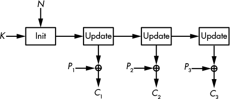
Figure 5-2: The stateful stream cipher

Counter-based stream ciphers produce chunks of keystream from a key, a nonce, and a counter value, as shown in Figure 5-3. Unlike stateful stream ciphers, such as Salsa20, no secret state is memorized during keystream generation.

Figure 5-3: The counter-based stream cipher

These two approaches define the high-level architecture of the stream cipher, regardless of how the core algorithms work. The internals of the stream cipher also fall into two categories, depending on the target platform of the cipher: hardware oriented and software oriented.

Hardware-Oriented Stream Ciphers

When cryptographers talk about hardware, they mean application-specific integrated circuits (ASICs), programmable logic devices (PLDs), and field-programmable gate arrays (FPGAs). A cipher’s hardware implementation is an electronic circuit that implements the cryptographic algorithm at the bit level and that can’t be used for anything else; in other words, the circuit is dedicated hardware. On the other hand, software implementations of cryptographic algorithms simply tell a microprocessor what instructions to execute in order to run the algorithm. These instructions operate on bytes or words and then call pieces of electronic circuit that implement general-purpose operations such as addition and multiplication. Software deals with bytes or words of 32 or 64 bits, whereas hardware deals with bits. The first stream ciphers worked with bits in order to save complex word-wise operations and thus be more efficient in hardware, their target platform at the time.

The main reason why stream ciphers were commonly used for hardware implementations is that they were cheaper than block ciphers. Stream ciphers needed less memory and fewer logical gates than block ciphers, and therefore occupied a smaller area on an integrated circuit, which reduced fabrication costs. For example, counting in gate-equivalents, the standard area metric for integrated circuits, you could find stream ciphers taking less than 1000 gate-equivalents; by contrast, typical software-oriented block ciphers needed at least 10000 gate-equivalents, making crypto an order of magnitude more expensive than with stream ciphers.

Today, however, block ciphers are no longer more expensive than stream ciphers—first, because there are now hardware-friendly block ciphers about as small as stream ciphers, and second, because the cost of hardware has plunged. Yet stream ciphers are often associated with hardware because they used to be the best option.

In the next section, I’ll explain the basic mechanism behind hardware stream ciphers, called feedback shift registers (FSRs). Almost all hardware stream ciphers rely on FSRs in some way, whether that’s the A5/1 cipher used in 2G mobile phones or the more recent cipher Grain-128a.

Feedback Shift Registers

Countless stream ciphers have used FSRs because they’re simple and well understood. An FSR is simply an array of bits equipped with an update feedback function, which I’ll denote as f. The FSR’s state is stored in the array, or register, and each update of the FSR uses the feedback function to change the state’s value and to produce one output bit.

In practice, an FSR works like this: if R₀ is the initial value of the FSR, the next state, R₁, is defined as R₀ left-shifted by 1 bit, where the bit leaving the register is returned as output, and where the empty position is filled with f(R₀).

The same rule is repeated to compute the subsequent state values R₂, R₃, and so on. That is, given R_t, the FSR’s state at time t, the next state, R_{t + 1}, is the following:

R_{i + 1} = (R_t << 1)|f(R_t)

In this equation, | is the logical OR operator and << is the shift operator, as used in the C language. For example, given the 8-bit string 00001111, we have this:

The bit shift moves the bits to the left, losing the leftmost bit in order to retain the state’s bit length, and zeroing the rightmost bit. The update operation of an FSR is identical, except that instead of being set to 0, the rightmost bit is set to f(R_t).

Consider, for example, a 4-bit FSR whose feedback function f XORs all 4 bits together. Initialize the state to the following:

1 1 0 0

Now shift the bits to the left, where 1 is output and the rightmost bit is set to the following:

f(1100) = 1 ⊕ 1 ⊕ 0 ⊕ 0 = 0

Now the state becomes this:

1 0 0 0

The next update outputs 1, left-shifts the state, and sets the rightmost bit to the following:

f(1000) = 1 ⊕ 0 ⊕ 0 ⊕0 = 1

Now the state is this:

0 0 0 1

The next three updates return three 0 bits and give the following state values:

We thus return to our initial state of 1100 after five iterations, and we can see that updating the state five times from any of the values observed throughout this cycle will return us to this initial value. We say that 5 is the period of the FSR given any one of the values 1100, 1000, 0001, 0011, or 0110. Because the period of this FSR is 5, clocking the register 10 times will yield twice the same 5-bit sequence. Likewise, if you clock the register 20 times, starting from 1100, the output bits will be 11000110001100011000, or four times the same 5-bit sequence of 11000. Intuitively, such repeating patterns should be avoided, and a longer period is better for security.

Figure 5-4 shows the structure of this cycle, along with the other cycles of that FSR, with each cycle shown as a circle whose dots represent a state of the register.

Figure 5-4: Cycles of the FSR whose feedback function XORs the 4 bits together

Indeed, this particular FSR has two other period-5 cycles—namely, {0100, 1001, 0010, 0101, 1010} and {1111, 1110, 1101, 1011, 0111}. Note that any given state can belong to only one cycle of states. Here, we have three cycles of five states each, covering 15 of all the 2⁴ = 16 possible values of our 4-bit register. The 16th possible value is 0000, which, as Figure 5-4 shows, is a period-1 cycle because the FSR will transform 0000 to 0000.

You’ve seen that an FSR is essentially a register of bits, where each update of the register outputs a bit (the leftmost bit of the register) and where a function computes the new rightmost bit of the register. (All other bits are left-shifted.) The period of an FSR, from some initial state, is the number of updates needed until the FSR enters the same state again. If it takes N updates to do so, the FSR will produce the same N bits again and again.

Linear Feedback Shift Registers

Linear feedback shift registers (LFSRs) are FSRs with a linear feedback function—namely, a function that’s the XOR of some bits of the state, such as the example of a 4-bit FSR in the previous section and its feedback function returning the XOR of the register’s 4 bits. Recall that in cryptography, linearity is synonymous with predictability and suggestive of a simple underlying mathematical structure. And, as you might expect, thanks to this linearity, LFSRs can be analyzed using notions like linear complexity, finite fields, and primitive polynomials—but I’ll skip the math details and just give you the essential facts.

The choice of which bits are XORed together is crucial for the period of the LFSR and thus for its cryptographic value. The good news is that we know how to select the position of the bits in order to guarantee a maximal period, of 2ⁿ – 1. Specifically, we take the indices of the bits, from 1 for the rightmost to n for the leftmost, and write the polynomial expression 1 + X + X ² + . . . + X ⁿ, where the term X ⁱ is only included if the ith bit is one of the bits XORed in the feedback function. The period is maximal if and only if that polynomial is primitive. To be primitive, the polynomial must have the following qualities:

• The polynomial must be irreducible, meaning that it can’t be factorized; that is, written as a product of smaller polynomials. For example, X + X ³ is not irreducible because it’s equal to (1 + X)(X + X²):

  (1 + X)(X + X²) = X + X² + X² + X³ = X + X³

• The polynomial must satisfy certain other mathematical properties that cannot be easily explained without nontrivial mathematical notions but are easy to test.

For example, Figure 5-5 shows a 4-bit LFSR with the feedback polynomial 1 + X + X ³ + X ⁴ in which the bits at positions 1, 3, and 4 are XORed together to compute the new bit set to L₁. However, this polynomial isn’t primitive because it can be factorized into (1 + X ³)(1 + X).

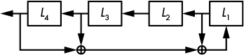
Figure 5-5: An LFSR with the feedback polynomial 1 + X + X³ + X⁴

Indeed, the period of the LFSR shown in Figure 5-5 isn’t maximal. To prove that, start from the state 0001.

0 0 0 1

Now left-shift by 1 bit and set the new bit to 0 + 0 + 1 = 1:

0 0 1 1

Repeating the operation four times gives the following state values:

And as you can see, the state after five updates is the same as the initial one, demonstrating that we’re in a period-5 cycle and proving that the LFSR’s period isn’t the maximal value of 15.

Now, by way of contrast, consider the LFSR shown in Figure 5-6.

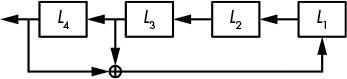
Figure 5-6: An LFSR with the feedback polynomial 1 + X³ + X⁴, a primitive polynomial, ensuring a maximal period

This feedback polynomial is a primitive polynomial described by 1 + X ³ + X ⁴, and you can verify that its period is indeed maximal (namely 15). Specifically, from an initial value, the state evolves as follows:

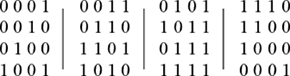
The state spans all possible values except 0000 with no repetition until it eventually loops. This demonstrates that the period is maximal and proves that the feedback polynomial is primitive.

Alas, using an LFSR as a stream cipher is insecure. If n is the LFSR’s bit length, an attacker needs only n output bits to recover the LFSR’s initial state, allowing them to determine all previous bits and predict all future bits. This attack is possible because the Berlekamp–Massey algorithm can be used to solve the equations defined by the LFSR’s mathematical structure to find not only the LFSR’s initial state but also its feedback polynomial. In fact, you don’t even need to know the exact length of the LFSR to succeed; you can repeat the Berlekamp–Massey algorithm for all possible values of n until you hit the right one.

The upshot is that LFSRs are cryptographically weak because they’re linear. Output bits and initial state bits are related by simple and short equations that can be easily solved with high-school linear algebra techniques.

To strengthen LFSRs, let’s thus add a pinch of nonlinearity.

Filtered LFSRs

Figure 5-7: A filtered LFSR

To mitigate the insecurity of LFSRs, you can hide their linearity by passing their output bits through a nonlinear function before returning them to produce what is called a filtered LFSR (see Figure 5-7).

The g function in Figure 5-7 must be a nonlinear function—one that both XORs bits together and combines them with logical AND or OR operations. For example, L₁L₂ + L₃L₄ is a nonlinear function (I’ve omitted the multiply sign, so L₁L₂ means L₁ × L₂, or L₁ & L₂ using C syntax).

Filtered LFSRs are stronger than plain LFSRs because their nonlinear function thwarts straightforward attacks. Still, more complex attacks such as the following will break the system:

• Algebraic attacks will solve the nonlinear equation systems deduced from the output bits, where unknowns in the equations are bits from the LFSR state.
• Cube attacks will compute derivatives of the nonlinear equations in order to reduce the degree of the system down to one and then solve it efficiently like a linear system.
• Fast correlation attacks will exploit filtering functions that, despite their nonlinearity, tend to behave like linear functions.

The lesson here, as we’ve seen in previous examples, is that Band-Aids don’t fix bullet holes. Patching a broken algorithm with a slightly stronger layer won’t make the whole thing secure. The problem has to be fixed at the core.

Nonlinear FSRs

Nonlinear FSRs (NFSRs) are like LFSRs but with a nonlinear feedback function instead of a linear one. That is, instead of just bitwise XORs, the feedback function can include bitwise AND and OR operations—a feature with both pros and cons.

One benefit of the addition of nonlinear feedback functions is that they make NFSRs cryptographically stronger than LFSRs because the output bits depend on the initial secret state in a complex fashion, according to equations of exponential size. The LFSRs’ linear function keeps the relations simple, with at most n terms (N₁, N₂, . . . , N_n, if the N_is are the NFSR’s state bits). For example, a 4-bit NFSR with an initial secret state (N₁, N₂, N₃, N₄) and a feedback function (N₁ + N₂ + N₁N₂ + N₃N₄) will produce a first output bit equal to the following:

N₁ + N₂ + N₁N₂ + N₃N₄

The second iteration replaces the N₁ value with that new bit. Expressing the second output bit in terms of the initial state, we get the following equation:

This new equation has algebraic degree 3 (the highest number of bits multiplied together, here in N₁N₃N₄) rather than degree 2 of the feedback function, and it has six terms instead of four. As a result, iterating the nonlinear function quickly yields unmanageable equations because the size of the output grows exponentially. Although you’ll never compute those equations when running the NFSR, an attacker would have to solve them in order to break the system.

One downside to NFSRs is that there’s no efficient way to determine an NFSR’s period, or simply to know whether its period is maximal. For an NFSR of n bits, you’d need to run close to 2ⁿ trials to verify that its period is maximal. This calculation is impossible for large NFSRs of 80 bits or more.

Fortunately, there’s a trick to using an NFSR without worrying about short periods: you can combine LFSRs and NFSRs to get both a guaranteed maximal period and the cryptographic strength—and that’s exactly how Grain-128a works.

Grain-128a

Remember the AES competition discussed in Chapter 4, in the context of the AES block cipher? The stream cipher Grain is the offspring of a similar project called the eSTREAM competition. This competition closed in 2008 with a shortlist of recommended stream ciphers, which included four hardware-oriented ciphers and four software-oriented ones. Grain is one of these hardware ciphers, and Grain-128a is an upgraded version from the original authors of Grain. Figure 5-8 shows the action mechanism of Grain-128a.

Figure 5-8: The mechanism of Grain-128a, with a 128-bit NFSR and a 128-bit LFSR

As you can see in Figure 5-8, Grain-128a is about as simple as a stream cipher can be, combining a 128-bit LFSR, a 128-bit NFSR, and a filter function, h. The LFSR has a maximal period of 2¹²⁸ – 1, which ensures that the period of the whole system is at least 2¹²⁸ – 1 to protect against potential short cycles in the NFSR. At the same time, the NFSR and the nonlinear filter function h add cryptographic strength.

Grain-128a takes a 128-bit key and a 96-bit nonce. It copies the 128 key bits into the NFSR’s 128 bits and copies the 96 nonce bits into the first 96 LFSR bits, filling the 32 bits left with ones and a single zero bit at the end. The initialization phase updates the whole system 256 times before returning the first keystream bit. During initialization, the bit returned by the h function is thus not output as a keystream, but instead goes into the LFSR to ensure that its subsequent state depends on both the key and the nonce.

Grain-128a’s LFSR feedback function is

f(L) = L₃₂ + L₄₇ + L₅₈ + L₉₀ + L₁₂₁ + L₁₂₈

where L₁, L₂, . . . , L₁₂₈ are the bits of the LFSR. This feedback function takes only 6 bits from the 128-bit LFSR, but that’s enough to get a primitive polynomial that guarantees a maximal period. The small number of bits minimizes the cost of a hardware implementation.

Here is the feedback polynomial of Grain-128a’s NFSR (N₁, . . . , N₁₂₈):

This function was carefully chosen to maximize its cryptographic strength while minimizing its implementation cost. It has an algebraic degree of 4 because its term with the most variables has four variables (namely, N₃₃N₃₅N₃₆N₄₀). Moreover, g can’t be approximated by a linear function because it is highly nonlinear. Also, in addition to g, Grain-128a XORs the bit coming out from the LFSRs to feed the result back as the NFSR’s new, rightmost bit.

The filter function h is another nonlinear function; it takes 9 bits from the NFSR and 7 bits from the LFSR and combines them in a way that ensures good cryptographic properties.

As I write this, there is no known attack on Grain-128a, and I’m confident that it will remain secure. Grain-128a is used in some low-end embedded systems that need a compact and fast stream cipher—typically industrial proprietary systems—which is why Grain-128a is little known in the open-source software community.

A5/1

A5/1 is a stream cipher that was used to encrypt voice communications in the 2G mobile standard. The A5/1 standard was created in 1987 but only published in the late 1990s after it was reverse engineered. Attacks appeared in the early 2000s, and A5/1 was eventually broken in a way that allows actual (rather than theoretical) decryption of encrypted communications. Let’s see why and how.

A5/1’s Mechanism

A5/1 relies on three LFSRs and uses a trick that looks clever at first glance but actually fails to be secure (see Figure 5-9).

Figure 5-9: The A5/1 cipher

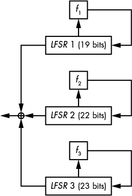
As you can see in Figure 5-9, A5/1 uses LFSRs of 19, 22, and 23 bits, with the polynomials for each as follows:

How could this be seen as secure with only LFSRs and no NFSR? The trick lies in A5/1’s update mechanism. Instead of updating all three LFSRs at each clock cycle, the designers of A5/1 added a clocking rule that does the following:

1. Checks the value of the ninth bit of LFSR 1, the 11th bit of LFSR 2, and the 11th bit of LFSR 3, called the clocking bits. Of those three bits, either all have the same value (1 or 0) or exactly two have the same value.

2. Clocks the registers whose clocking bits are equal to the majority value, 0 or 1. Either two or three LFSRs are clocked at each update.

Without this simple rule, A5/1 would provide no security whatsoever, and bypassing this rule is enough to break the cipher. However, that is easier said than done, as you’ll see.

2G communications use A5/1 with a key of 64 bits and a 22-bit nonce, which is changed for every new data frame. Attacks on A5/1 recover the 64-bit initial state of the system (the 19 + 22 + 23 LFSR initial value), thus in turn revealing the nonce (if it was not already known) and the key, by unwinding the initialization mechanism. The attacks are referred to as known-plaintext attacks (KPAs) because part of the encrypted data is known, which allows attackers to determine the corresponding keystream parts by XORing the ciphertext with the known plaintext chunks.

There are two main types of attacks on A5/1:

Subtle attacks Exploit the internal linearity of A5/1 and its simple irregular clocking system

Brutal attacks Only exploit the short key of A5/1 and the invertibility of the frame number injection

Let’s see how these attacks work.

Subtle Attacks

In a subtle attack called a guess-and-determine attack, an attacker guesses certain secret values of the state in order to determine others. In cryptanalysis, “guessing” means brute-forcing: for each possible value of LFSRs 1 and 2, and all possible values of LFSR 3’s clocking bit during the first 11 clocks, the attack reconstructs LFSR 3’s bits by solving equations that depend on the bits guessed. When the guess is correct, the attacker gets the right value for LFSR 3.

The attack’s pseudocode looks like this:

For all 2¹⁹ values of LFSR 1's initial state
    For all 2²² values of LFSR 2's initial state
        For all 2¹¹ values of LFSR 3's clocking bit during the first 11 clocks
            Reconstruct LFSR 3's initial state
            Test whether guess is correct; if yes, return; else continue

How efficient is this attack compared to the 2⁶⁴-trial brute-force search discussed in Chapter 3? This attack makes at most 2¹⁹ × 2²² × 2¹¹ = 2⁵² operations in the worst case, when the algorithm only succeeds at the very last test. That’s 2¹² (or about 4000) times faster than in the brute-force search, assuming that the last two operations in the above pseudocode require about as much computation as testing a 64-bit key in a brute-force search. But is this assumption correct?

Recall our discussion of the full attack cost in Chapter 3. When evaluating the cost of an attack, we need to consider not only the amount of computation required to perform the attack but also parallelism and memory consumption. Neither are issues here: as with any brute-force attack, the guess-and-determine attack is embarrassingly parallel (or N times faster when run on N cores) and doesn’t need more memory than just running the cipher itself.

Our 2⁵² attack cost estimate is inaccurate for another reason. In fact, each of the 2⁵² operations (testing a key candidate) takes about four times as many clock cycles as does testing a key in a brute-force attack. The upshot is that the real cost of this particular attack is closer to 4 × 2⁵² = 2⁵⁴ operations, when compared to a brute-force attack.

The guess-and-determine attack on A5/1 can decrypt encrypted mobile communications, but it takes a couple of hours to recover the key when run on a cluster of dedicated hardware devices. In other words, it’s nowhere near real-time decryption. For that, we have another type of attack.

Brutal Attacks

The time-memory trade-off (TMTO) attack is the brutal attack on A5/1. This attack doesn’t care about A5/1’s internals; it cares only that its state is 64 bits long. The TMTO attack sees A5/1 as a black box that takes in a 64-bit value (the state) and spits out a 64-bit value (the first 64 keystream bits).

The idea behind the attack is to reduce the cost of a brute-force search in exchange for using lots of memory. The simplest type of TMTO is the codebook attack. In a codebook attack, you precompute a table of 2⁶⁴ elements containing a combination of key and value pairs (key:value), and store the output value for each of the 2⁶⁴ possible keys. To use this precomputed table for the attack, you simply collect the output of an A5/1 instance and then look up in the table which key corresponds to that output. The attack itself is fast—taking only the amount of time necessary to look up a value in memory—but the creation of the table takes 2⁶⁴ computations of A5/1. Worse, codebook attacks require an insane amount of memory: 2⁶⁴ × (64 + 64) bits, which is 2⁶⁸ bytes or 256 exabytes. That’s dozens of data centers, so we can forget about it.

TMTO attacks reduce the memory required by a codebook attack at the price of increased computation during the online phase of the attack; the smaller the table, the more computations required to crack a key. Regardless, it will still cost about 2⁶⁴ operations to prepare the table, but that needs to be done only once.

In 2010, researchers took about two months to generate two terabytes’ worth of tables, using graphics processing units (GPUs) and running 100000 instances of A5/1 in parallel. With the help of such large tables, calls encrypted with A5/1 could be decrypted almost in real time. Telecommunication operators have implemented workarounds to mitigate the attack, but a real solution came with the later 3G and 4G mobile telephony standards, which ditched A5/1 altogether.

Software-Oriented Stream Ciphers

Software stream ciphers work with bytes or 32- or 64-bit words instead of individual bits, which proves to be more efficient on modern CPUs where instructions can perform arithmetic operations on a word in the same amount of time as on a bit. Software stream ciphers are therefore better suited than hardware ciphers for servers or browsers running on personal computers, where powerful general-purpose processors run the cipher as native software.

Today, there is considerable interest in software stream ciphers for a few reasons. First, because many devices embed powerful CPUs and hardware has become cheaper, there’s less of a need for small bit-oriented ciphers. For example, the two stream ciphers in the mobile communications standard 4G (the European SNOW3G and the Chinese ZUC) work with 32-bit words and not bits, unlike the older A5/1.

Second, stream ciphers have gained popularity in software at the expense of block ciphers, notably following the fiasco of the padding oracle attack against block ciphers in CBC mode. In addition, stream ciphers are easier to specify and to implement than block ciphers: instead of mixing message and key bits together, stream ciphers just ingest key bits as a secret. In fact, one of the most popular stream ciphers is actually a block cipher in disguise: AES in counter mode (CTR).

One software stream cipher design, used by SNOW3G and ZUC, copies hardware ciphers and their FSRs, replacing bits with bytes or words. But these aren’t the most interesting designs for a cryptographer. As of this writing, the two designs of most interest are RC4 and Salsa20, which are used in numerous systems, despite the fact that one is completely broken.

RC4

Designed in 1987 by Ron Rivest of RSA Security, then reverse engineered and leaked in 1994, RC4 has long been the most widely used stream cipher. RC4 has been used in countless applications, most famously in the first Wi-Fi encryption standard Wireless Equivalent Privacy (WEP) and in the Transport Layer Security (TLS) protocol used to establish HTTPS connections. Unfortunately, RC4 isn’t secure enough for most applications, including WEP and TLS. To understand why, let’s see how RC4 works.

How RC4 Works

RC4 is among the simplest ciphers ever created. It doesn’t perform any crypto-like operations, and it has no XORs, no multiplications, no S-boxes . . . nada. It simply swaps bytes. RC4’s internal state is an array, S, of 256 bytes, first set to S[0] = 0, S[1] = 1, S[2] = 2, . . . , S[255] = 255, and then initialized from an n-byte K using its key scheduling algorithm (KSA), which works as shown in the Python code in Listing 5-1.

j = 0
# set S to the array S[0] = 0, S[1] = 1, . . . , S[255] = 255
S = range(256)
# iterate over i from 0 to 255
for i in range(256):
    # compute the sum of v
    j = (j + S[i] + K[i % n]) % 256
    # swap S[i] and S[j]
    S[i], S[j] = S[j], S[i]

Listing 5-1: The key scheduling algorithm of RC4

Once this algorithm completes, array S still contains all the byte values from 0 to 255, but now in a random-looking order. For example, with the all-zero 128-bit key, the state S (from S[0] to S[255]) becomes this:

0, 35, 3, 43, 9, 11, 65, 229, (. . .), 233, 169, 117, 184, 31, 39

However, if I flip the first key bit and run the KSA again, I get a totally different, apparently random state:

32, 116, 131, 134, 138, 143, 149, (. . .), 152, 235, 111, 48, 80, 12

Given the initial state S, RC4 generates a keystream, KS, of the same length as the plaintext, P, in order to compute a ciphertext: C = P ⊕ KS. The bytes of the keystream KS are computed from S according to the Python code in Listing 5-2, if P is m bytes long.

i = 0
j = 0
for b in range(m):
    i = (i + 1) % 256
    j = (j + S[i]) % 256
    S[i], S[j] = S[j], S[i]
    KS[b] = S[(S[i] + S[j]) % 256]

Listing 5-2: The keystream generation of RC4, where S is the state initialized in Listing 5-1

In Listing 5-2, each iteration of the for loop modifies up to 2 bytes of RC4’s internal state S: the S[i] and S[j] whose values are swapped. That is, if i = 0 and j = 4, and if S[0] = 56 and S[4] = 78, then the swap operation sets S[0] to 78 and S[4] to 56. If j equals i, then S[i] isn’t modified.

This looks too simple to be secure, yet it took 20 years for cryptanalysts to find exploitable flaws. Before the flaws were revealed, we only knew RC4’s weaknesses in specific implementations, as in the first Wi-Fi encryption standard, WEP.

RC4 in WEP

WEP, the first generation Wi-Fi security protocol, is now completely broken due to weaknesses in the protocol’s design and in RC4.

In its WEP implementation, RC4 encrypts payload data of 802.11 frames, the datagrams (or packets) that transport data over the wireless network. All payloads delivered in the same session use the same secret key of 40 or 104 bits but have what is a supposedly unique 3-byte nonce encoded in the frame header (the part of the frame that encodes metadata and comes before the actual payload). See the problem?

The problem is that RC4 doesn’t support a nonce, at least not in its official specification, and a stream cipher can’t be used without a nonce. The WEP designers addressed this limitation with a workaround: they included a 24-bit nonce in the wireless frame’s header and prepended it to the WEP key to be used as RC4’s secret key. That is, if the nonce is the bytes N[0], N[1], N[2] and the WEP key is K[0], K[1], K[2], K[3], K[4], the actual RC4 key is N[0], N[1], N[2], K[0], K[1], K[2], K[3], K[4]. The net effect is to have 40-bit secret keys yield 64-bit effective keys, and 104-bit keys yield 128-bit effective keys. The result? The advertised 128-bit WEP protocol actually offers only 104-bit security, at best.

But here are the real problems with WEP’s nonce trick:

• The nonces are too small at only 24 bits. This means that if a nonce is chosen randomly for each new message, you’ll have to wait about 2^24/2 = 2¹² packets, or a few megabytes’ worth of traffic, until you can find two packets encrypted with the same nonce, and thus the same keystream. Even if the nonce is a counter running from 0 to 2²⁴ – 1, it will take a few gigabytes’ worth of data until a rollover, when the repeated nonce can allow the attacker to decrypt packets. But there’s a bigger problem.
• Combining the nonce and key in this fashion helps recover the key. WEP’s three non-secret nonce bytes let an attacker determine the value of S after three iterations of the key scheduling algorithm. Because of this, cryptanalysts found that the first keystream byte strongly depends on the first secret key byte—the fourth byte ingested by the KSA—and that this bias can be exploited to recover the secret key.

Exploiting those weaknesses requires access to both ciphertexts and the keystream; that is, known or chosen plaintexts. But that’s easy enough: known plaintexts occur when the Wi-Fi frames encapsulate data with a known header, and chosen plaintexts occur when the attacker injects known plaintext encrypted with the target key. The upshot is that the attacks work in practice, not just on paper.

Following the appearance of the first attacks on WEP in 2001, researchers found faster attacks that required fewer ciphertexts. Today, you can even find tools such as aircrack-ng that implement the entire attack, from network sniffing to cryptanalysis.

WEP’s insecurity is due to both weaknesses in RC4, which takes a single one-use key instead of a key and nonce (as in any decent stream cipher), and weaknesses in the WEP design itself.

Now let’s look at the second biggest failure of RC4.

RC4 in TLS

TLS is the single most important security protocol used on the internet. It is best known for underlying HTTPS connections, but it’s also used to protect some virtual private network (VPN) connections, as well as email servers, mobile applications, and many others. And sadly, TLS has long supported RC4.

Unlike WEP, the TLS implementation doesn’t make the same blatant mistake of tweaking the RC4 specs in order to use a public nonce. Instead, TLS just feeds RC4 a unique 128-bit session key, which means it’s a bit less broken than WEP.

The weakness in TLS is due only to RC4 and its inexcusable flaws: statistical biases, or non-randomness, which we know is a total deal breaker for a stream cipher. For example, the second keystream byte produced by RC4 is zero, with a probability of 1/128, whereas it should be 1/256 ideally. (Recall that a byte can take 256 values from 0 to 255; hence, a truly random byte is zero with a chance of 1/256.) Crazier still is the fact that most experts continued to trust RC4 as late as 2013, even though its statistical biases have been known since 2001.

RC4’s known statistical biases should have been enough to ditch the cipher altogether, even if we didn’t know how to exploit the biases to compromise actual applications. In TLS, RC4’s flaws weren’t publicly exploited until 2011, but the NSA allegedly managed to exploit RC4’s weaknesses to compromise TLS’s RC4 connections well before then.

As it turned out, not only was RC4’s second keystream byte biased, but all of the first 256 bytes were biased as well. In 2011, researchers found that the probability that one of those bytes comes to zero equals 1/256 + c/256², for some constant, c, taking values between 0.24 and 1.34. It’s not just for the byte zero but for other byte values as well. The amazing thing about RC4 is that it fails where even many noncryptographic PRNGs succeed—namely, at producing uniformly distributed pseudorandom bytes (that is, where each of the 256 bytes has a chance of 1/256 of showing up).

Even the weakest attack model can be used to exploit RC4’s flawed TLS implementation: basically, you collect ciphertexts and look for the plaintext, not the key. But there’s a caveat: you’ll need many ciphertexts, encrypting the same plaintext several times using different secret keys. This attack model is sometimes called the broadcast model, because it’s akin to broadcasting the same message to multiple recipients.

For example, say you want to decrypt the plaintext byte P₁ given many ciphertext bytes obtained by intercepting the different ciphertexts of the same message. The first four ciphertext bytes will therefore look like this:

Because of RC4’s bias, keystream bytes KS₁ⁱ are more likely to be zero than any other byte value. Therefore, C₁ⁱ bytes are more likely to be equal to P₁ than to any other value. In order to determine P₁ given the C₁ⁱ bytes, you simply count the number of occurrences of each byte value and return the most frequent one as P₁. However, because the statistical bias is very small, you’ll need millions of values to get it right with any certainty.

The attack generalizes to recover more than one plaintext byte and to exploit more than one biased value (zero here). The algorithm just becomes a bit more complicated. However, this attack is hard to put into practice because it needs to collect many ciphertexts encrypting the same plaintext but using different keys. For example, the attack can’t break all TLS-protected connections that use RC4 because you need to trick the server into encrypting the same plaintext to many different recipients, or many times to the same recipient with different keys.

Salsa20

Salsa20 is a simple, software-oriented cipher optimized for modern CPUs that has been implemented in numerous protocols and libraries, along with its variant, ChaCha. Its designer, respected cryptographer Daniel J. Bernstein, submitted Salsa20 to the eSTREAM competition in 2005 and won a place in eSTREAM’s software portfolio. Salsa20’s simplicity and speed have made it popular among developers.

Figure 5-10: Salsa20’s encryption scheme for a 512-bit plaintext block

Salsa20 is a counter-based stream cipher—it generates its keystream by repeatedly processing a counter incremented for each block. As you can see in Figure 5-10, the Salsa20 core algorithm transforms a 512-bit block using a key (K), a nonce (N), and a counter value (Ctr). Salsa20 then adds the result to the original value of the block to produce a keystream block. (If the algorithm were to return the core’s permutation directly as an output, Salsa20 would be totally insecure, because it could be inverted. The final addition of the initial secret state K || N || Ctr makes the transform key-to-keystream-block non-invertible.)

The Quarter-Round Function

Salsa20’s core permutation uses a function called quarter-round (QR) to transform four 32-bit words (a, b, c, and d), as shown here:

These four lines are computed from top to bottom, meaning that the new value of b depends on a and d, the new value of c depends on a and on the new value of b (and thus d as well), and so on.

The operation <<< is wordwise left-rotation by the specified number of bits, which can be any value between 1 and 31 (for 32-bit words). For example, <<< 8 rotates a word’s bits of eight positions toward the left, as shown in these examples:

Transforming Salsa20’s 512-bit State

Salsa20’s core permutation transforms a 512-bit internal state viewed as a 4 × 4 array of 32-bit words. Figure 5-11 shows the initial state, using a key of eight words (256 bits), a nonce of two words (64 bits), a counter of two words (64 bits), and four fixed constant words (128 bits) that are identical for each encryption/decryption and all blocks.

To transform the initial 512-bit state, Salsa20 first applies the QR transform to all four columns independently (known as the column-round) and then to all four rows independently (the row-round), as shown in Figure 5-12. The sequence column-round/row-round is called a double-round. Salsa20 repeats 10 double-rounds, for 20 rounds in total, thus the 20 in Salsa20.

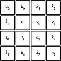
Figure 5-11: The initialization of Salsa20’s state

Figure 5-12: Columns and rows transformed by Salsa20’s quarter-round (QR) function

The column-round transforms the four columns like so:

The row-round transforms the rows by doing the following:

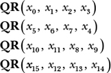
Notice that in a column-round, each QR takes x_i arguments ordered from the top to the bottom line, whereas a row-round’s QR takes as a first argument the words on the diagonal (as shown in the array on the right in Figure 5-12) rather than words from the first column.

Evaluating Salsa20

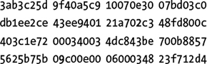
Listing 5-3 shows Salsa20’s initial states for the first and second blocks when initialized with an all-zero key (00 bytes) and an all-one nonce (ff bytes). These two states differ in only one bit, in the counter, as shown in bold: specifically, 0 for the first block and 1 for the second.

61707865 00000000 00000000 00000000      61707865 00000000 00000000 00000000
00000000 3320646e ffffffff ffffffff      00000000 3320646e ffffffff ffffffff
00000000 00000000 79622d32 00000000      00000001 00000000 79622d32 00000000
00000000 00000000 00000000 6b206574      00000000 00000000 00000000 6b206574

Listing 5-3: Salsa20’s initial states for the first two blocks with an all-zero key and an all-one nonce

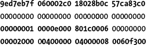
Yet, despite only a one-bit difference, the respective internal states after 10 double-rounds are totally different from each other, as Listing 5-4 shows.

e98680bc f730ba7a 38663ce0 5f376d93      1ba4d492 c14270c3 9fb05306 ff808c64
85683b75 a56ca873 26501592 64144b6d      b49a4100 f5d8fbbd 614234a0 e20663d1
6dcb46fd 58178f93 8cf54cfe cfdc27d7      12e1e116 6a61bc8f 86f01bcb 2efead4a
68bbe09e 17b403a1 38aa1f27 54323fe0      77775a13 d17b99d5 eb773f5b 2c3a5e7d

Listing 5-4: The states from Listing 5-3 after 10 Salsa20 double-rounds

But remember, even though word values in the keystream block may look random, we’ve seen that it’s far from a guarantee of security. RC4’s output looks random, but it has blatant biases. Fortunately, Salsa20 is much more secure than RC4 and doesn’t have statistical biases.

Differential Cryptanalysis

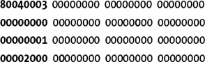
To demonstrate why Salsa20 is more secure than RC4, let’s have a look at the basics of differential cryptanalysis, the study of the differences between states rather than their actual values. For example, the two initial states in Figure 5-13 differ by one bit in the counter, or by the word x₈ in the Salsa20 state array. The bitwise difference between these two states is thus shown in this array:

The difference between the two states is actually the XOR of these states. The 1 bit shown in bold corresponds to a 1-bit difference between the two states. In the XOR of the two states, any nonzero bits indicate differences.

To see how fast changes propagate in the initial state as a result of Salsa20’s core algorithm, let’s look at the difference between two states throughout the rounds iteration. After one round, the difference propagates across the first column to two of the three other words in that column:

After two rounds, differences further propagate across the rows that already include a difference, which is all but the second row. At this point the differences between the states are rather sparse; not many bits have changed within a word as shown here:

After three rounds, the differences between the states become more dense, though the many zero nibbles indicate that many bit positions are still not affected by the initial difference:

After four rounds, differences look random to a human observer, and they are also almost random statistically as well, as shown here:

So after only four rounds, a single difference propagates to most of the bits in the 512-bit state. In cryptography, this is called full diffusion.

We’ve seen that differences propagate quickly throughout Salsa20 rounds. But not only do differences propagate across all states, they also do so according to complex equations that make future differences hard to predict because highly nonlinear relations drive the state’s evolution, thanks to the mix of XOR, addition, and rotation. If only XORs were used, we’d still have many differences propagating, but the process would be linear and therefore insecure.

Attacking Salsa20/8

Salsa20 makes 20 rounds by default, but it’s sometimes used with only 12 rounds, in a version called Salsa20/12, to make it faster. Although Salsa20/12 uses eight fewer rounds than Salsa20, it’s still significantly stronger than the weaker Salsa20/8, another version with eight rounds, which is more rarely used.

Breaking Salsa20 should ideally take 2²⁵⁶ operations, thanks to its use of a 256-bit key. If the key can be recovered by performing any fewer than 2²⁵⁶ operations, the cipher is in theory broken. That’s exactly the case with Salsa20/8.

The attack on Salsa20/8 (published in the 2008 paper New Features of Latin Dances: Analysis of Salsa, ChaCha, and Rumba, of which I’m a co-author, and for which we won a cryptanalysis prize from Daniel J. Bernstein) exploits a statistical bias in Salsa’s core algorithm after four rounds to recover the key of eight-round Salsa20. In reality, this is mostly a theoretical attack: we estimate its complexity at 2²⁵¹ operations of the core function—impossible, but less so than breaking the expected 2²⁵⁶ complexity.

The attack exploits not only a bias over the first four rounds of Salsa20/8, but also a property of the last four rounds: knowing the nonce, N, and the counter, Ctr (refer back to Figure 5-10), the only value needed to invert the computation from the keystream back to the initial state is the key, K. But as shown in Figure 5-13, if you only know some part of K, you can partially invert the computation up until the fourth round and observe some bits of that intermediate state—including the biased bit! You’ll only observe the bias if you have the correct guess of the partial key; hence, the bias serves as an indicator that you’ve got the correct key.

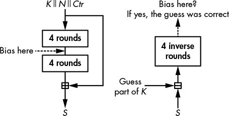
Figure 5-13: The principle of the attack on Salsa20/8

In the actual attack on Salsa20/8, in order to determine the correct guess, we need to guess 220 bits of the key, and we need 2³¹ pairs of keystream blocks, all with the same specific difference in the nonce. Once we’ve singled out the correct 220 bits, we simply need to brute-force 36 bits. The brute-forcing takes 2³⁶ operations, a computation that dwarfs the unrealistic 2²²⁰ × 2³¹ = 2²⁵¹ trials needed to find the 220 bits to complete the first part of the attack.

How Things Can Go Wrong

Alas, many things can go wrong with stream ciphers, from brittle, insecure designs to strong algorithms incorrectly implemented. I’ll explore each category of potential problems in the following sections.

Nonce Reuse

The most common failure seen with stream ciphers is an amateur mistake: it occurs when a nonce is reused more than once with the same key. This produces identical keystreams, allowing you to break the encryption by XORing two ciphertexts together. The keystream then vanishes, and you’re left with the XOR of the two plaintexts.

For example, older versions of Microsoft Word and Excel used a unique nonce for each document, but the nonce wasn’t changed once the document was modified. As a result, the clear and encrypted text of an older version of a document could be used to decrypt later encrypted versions. If even Microsoft made this kind of blunder, you can imagine how large the problem might be.

Certain stream ciphers designed in the 2010s tried to mitigate the risk of nonce reuse by building “misuse-resistant” constructions, or ciphers that remain secure even if a nonce is used twice. However, achieving this level of security comes with a performance penalty, as we’ll see in Chapter 8 with the SIV mode.

Broken RC4 Implementation

Though it’s already weak, RC4 can become even weaker if you blindly optimize its implementation. For example, consider the following entry in the 2007 Underhanded C Contest, an informal competition where programmers write benign-looking code that actually includes a malicious function.

Here’s how it works. The naive way to implement the line swap(S[i], S[j]) in RC4’s algorithm is to do the following, as expressed in this Python code:

buf = S[i]
S[i] = S[j]
S[j] = buf

This way of swapping two variables obviously works, but you need to create a new variable, buf. To avoid this, programmers often use the XOR-swap trick, shown here, to swap the values of the variables x and y:

x = x ⊕ y
y = x ⊕ y
x = x ⊕ y

This trick works because the second line sets y to x ⊕ y ⊕ y = x, and the third line sets x to x ⊕ y ⊕ x ⊕ y ⊕ y = y. Using this trick to implement RC4 gives the implementation shown in Listing 5-5 (adapted from Wagner and Biondi’s program submitted to the Underhanded C Contest, and online at http://www.underhanded-c.org/_page_id_16.html).

# define TOBYTE(x) (x) & 255
# define SWAP(x,y) do { x^=y; y^=x; x^=y; } while (0)
static unsigned char S[256];
static int i=0, j=0;

void init(char *passphrase) {
    int passlen = strlen(passphrase);
    for (i=0; i<256; i++)
        S[i] = i;
    for (i=0; i<256; i++) {
        j = TOBYTE(j + S[TOBYTE(i)] + passphrase[j % passlen]);
        SWAP(S[TOBYTE(i)], S[j]);
    }
    i = 0; j = 0;
}

unsigned char encrypt_one_byte(unsigned char c) {
    int k;
    i = TOBYTE(i+1);
    j = TOBYTE(j + S[i]);
    SWAP(S[i], S[j]);
    k = TOBYTE(S[i] + S[j]);
    return c ^ S[k];
}

Listing 5-5: Incorrect C implementation of RC4, due to its use of an XOR swap

Now stop reading, and try to spot the problem with the XOR swap in Listing 5-5.

Things will go south when i = j. Instead of leaving the state unchanged, the XOR swap will set S[i] to S[i] ⊕ S[i] = 0. In effect, a byte of the state will be set to zero each time i equals j in the key schedule or during encryption, ultimately leading to an all-zero state and thus to an all-zero keystream. For example, after 68KB of data have been processed, most of the bytes in the 256-byte state are zero, and the output keystream looks like this:

00 00 00 00 00 00 00 53 53 00 00 00 00 00 00 00 00 00 00 00 13 13 00 5c 00 a5 00 00 . . .

The lesson here is to refrain from over-optimizing your crypto implementations. Clarity and confidence always trump performance in cryptography.

Weak Ciphers Baked Into Hardware

When a cryptosystem fails to be secure, some systems can quickly respond by silently updating the affected software remotely (as with some pay-TV systems) or by releasing a new version and prompting the users to upgrade (as with mobile applications). Some other systems are not so lucky and need to stick to the compromised cryptosystem for a while before upgrading to a secure version, as is the case with certain satellite phones.

In the early 2000s, US and European telecommunication standardization institutes (TIA and ETSI) jointly developed two standards for satellite phone (satphone) communications. Satphones are like mobile phones, except that their signal goes through satellites rather than terrestrial stations. The advantage is that you can use them pretty much everywhere in the world. Their downsides are the price, quality, latency, and, as it turns out, security.

GMR-1 and GMR-2 are the two satphone standards adopted by most commercial vendors, such as Thuraya and Inmarsat. Both include stream ciphers to encrypt voice communications. GMR-1’s cipher is hardware oriented, with a combination of four LFSRs, similar to A5/2, the deliberately insecure cipher in the 2G mobile standard aimed at non-Western countries. GMR-2’s cipher is software oriented, with an 8-byte state and the use of S-boxes. Both stream ciphers are insecure, and will only protect users against amateurs, not against state agencies.

This story should remind us that stream ciphers used to be easier to break than block ciphers and that they’re easier to sabotage. Why? Well, if you design a weak stream cipher on purpose, when the flaw is found, you can still blame it on the weakness of stream ciphers and deny any malicious intent.

Further Reading

To learn more about stream ciphers, begin with the archives of the eSTREAM competition at http://www.ecrypt.eu.org/stream/project.html, where you’ll find hundreds of papers on stream ciphers, including details of more than 30 candidates and many attacks. Some of the most interesting attacks are the correlation attacks, algebraic attacks, and cube attacks. See in particular the work of Courtois and Meier for the first two attack types and that of Dinur and Shamir for cube attacks.

For more information on RC4, see the work of Paterson and his team at http://www.isg.rhul.ac.uk/tls/ on the security of RC4 as used in TLS and WPA. Also see Spritz, the RC4-like cipher created in 2014 by Rivest, who designed RC4 in the 1980s.

Salsa20’s legacy deserves your attention, too. The stream cipher ChaCha is similar to Salsa20, but with a slightly different core permutation that was later used in the hash function BLAKE, as you’ll see in Chapter 6. These algorithms all leverage Salsa20’s software implementation techniques using parallelized instructions, as discussed at https://cr.yp.to/snuffle.html.