
7 Building a scheduling service for ad hoc tasks
- Approaching architectural decisions when faced with a novel problem
- Defining nonfunctional requirements
- Choosing the right AWS service to satisfy nonfunctional requirements
- Combining different AWS services
With serverless technologies, you can build scalable and resilient applications quickly by offloading infrastructure responsibilities to AWS. Doing so allows you to focus on the needs of your customers and your business. Ideally, all the code you write is directly attributed to features that differentiate your business and add value for your customers.
What this means in practice is that you use many managed services instead of building and running your own. For example, instead of running a cluster of RabbitMQ servers on EC2, you use Amazon Simple Queue Service (SQS). Throughout the course of this book, you have also read about other AWS services such as DynamoDB and Step Functions.
Therefore, an important skill is to be able to analyze the nonfunctional requirements of a system and choose the correct AWS service to work with. But the AWS ecosystem is enormous and consists of a huge number of different services. Many of these services overlap in their use cases but have different operational constraints and scaling characteristics. For example, to add a queue between two Lambda functions to decouple them, you can use any of the following services:
These services have different characteristics when it comes to their scaling behavior, cost, service limits, and how they integrate with Lambda. Depending on your requirements, some might be a better fit for you than others.
Although AWS gives you a lot of different services to architect your system, it doesn’t offer any guidance or opinion on when to use which. As a developer or architect working with AWS, one of the most challenging tasks is figuring this out for yourself.
This chapter shines a light on the problem by taking you through the design process for a scheduling service for ad hoc tasks. It’s a common need for applications, and AWS does not yet offer a managed service to solve this problem. The closest thing in AWS is the scheduled events in EventBridge, but scheduling repeated tasks (e.g., do X every Y seconds) is different than scheduling ad hoc tasks (e.g., do X at 2021-08-30T23:59:59Z, do Y at 2021-08-20T08:05:00Z).
The functional requirement for such a scheduling service is simple: you schedule an ad hoc task to be run at a specified date and time (for example, “Remind me to call mum on Monday, at 9:00”). What’s interesting about this is that it has to deal with different nonfunctional requirements depending on the application (for example, “It needs to handle a million open tasks that are scheduled but not yet run”).
For the rest of this chapter, you will see five different solutions for this scheduling service using different AWS services and learn how to evaluate them. But first, let’s define the nonfunctional requirements that we will evaluate the solutions against. Here is the plan for this chapter:
-
Define nonfunctional requirements. The four nonfunctional requirements we will consider are precision, scalability (number of open tasks), scalability (hotspots), and cost. All the following solutions will be evaluated against these requirements:
-
-
Cron with EventBridge—A simple solution using cron jobs to find open tasks and run them.
-
DynamoDB TTL—A creative use of DynamoDB’s time-to-live (TTL) mechanism to trigger and run the scheduled ad hoc tasks.
-
Step Functions—A solution that uses Step Function’s Wait state to schedule and run tasks.
-
SQS—A solution that uses SQS’s DelaySeconds and VisibilityTimeout settings to hide tasks until their scheduled execution time.
-
Combining DynamoDB TTL and SQS—A solution that combines DynamoDB TTL with SQS to compensate for each other’s shortcomings.
-
-
Choose the right solution for your application. Different applications have different needs, and some nonfunctional requirements may be more important than others. In this section, you will see three different applications, understand their needs, and pick the most appropriate solution for them.
7.1 Defining nonfunctional requirements
The ad hoc scheduling service is an interesting problem that often shows up in different contexts and has different nonfunctional requirements. For example, a dating app may require ad hoc tasks to remind users a date is coming up. A multiplayer game may need to schedule ad hoc tasks to start or stop a tournament. A news site might use ad hoc tasks to cancel expired subscriptions.
User behaviors and traffic patterns differ between these contexts, which in turn create different nonfunctional requirements the service needs to meet. It’s important for you to define these requirements up front to prevent unconscious biases (such as a confirmation bias) from creeping in.
Too often, we subconsciously put more weight behind characteristics that align with our solution, even if they aren’t as important to our application. Defining requirements up front helps us maintain our objectivity. For a service that allows you to schedule ad hoc tasks to run at a specific time, the following lists some nonfunctional requirements you need to consider:
-
Scalability (number of open tasks)—Can the service support millions of tasks that are scheduled but not yet processed?
-
Scalability (hotspots)—Can the service run millions of tasks at the same time?
Throughout this chapter, you will evaluate five different solutions against this set of nonfunctional requirements. And remember, there are no wrong answers! The goal of this chapter is to help you hone the skill of thinking through solutions and evaluating them. We’ll spend the rest of the chapter looking at these different solutions. Each provides a different approach and utilizes different AWS services. However, every solution uses only serverless components, and there is no infrastructure to manage. The five solutions include
After each solution, we’ll ask you to score the solution against the aforementioned nonfunctional requirements. You can compare your scores against ours and see the rationale for our scores. Let’s start with the solution for a cron job with EventBridge.
7.2 Cron job with EventBridge
This solution uses a cron job in EventBridge to invoke a Lambda function every couple of minutes (figure 7.1). With this solution, you will need the following:
-
A database (such as DynamoDB) to store all the scheduled tasks, including when they should run
-
A Lambda function that reads overdue tasks from the database and runs them

Figure 7.1 High-level architecture showing an EventBridge cron job with Lambda to run ad hoc scheduled tasks.
There are a few things to note about this solution:
-
The lowest granularity for an EventBridge schedule is 1 minute. Assuming the service is able to keep up with the rate of scheduled tasks that need to run, the precision of this solution is within 1 minute.
-
The Lambda function can run for up to 15 minutes. If the Lambda function fetches more scheduled tasks than it can process in 1 minute, then it can keep running until it completes the batch. In the meantime, the cron job can start another concurrent execution of this function. Therefore, you need to take care to avoid the same scheduled tasks being fetched and run twice.
-
The precision of individual tasks within the batch can vary, depending on their relative position in the batch and when they are actually processed. In the case of a large batch that cannot be processed within 1 minute, the precision for some tasks may be longer than 1 minute (figure 7.2).

Figure 7.2 The precision of individual tasks inside a batch can vary greatly depending on their position inside the batch.
-
It’s possible to increase the throughput of this solution by adding a Lambda function as the target multiple times (figure 7.3).
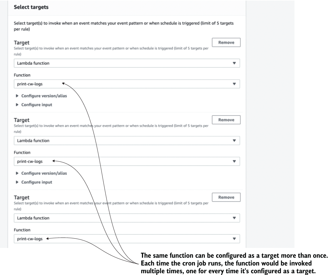
Figure 7.3 You can add the same Lambda function as a target for an EventBridge rule multiple times.
-
Because EventBridge has a limit of five targets per rule, you can use this technique to increase the throughput fivefold. This means every time the cron job runs, it creates five concurrent executions of this Lambda function. To avoid them all picking up and running the same tasks, you can configure different inputs for each target as figure 7.4 shows.
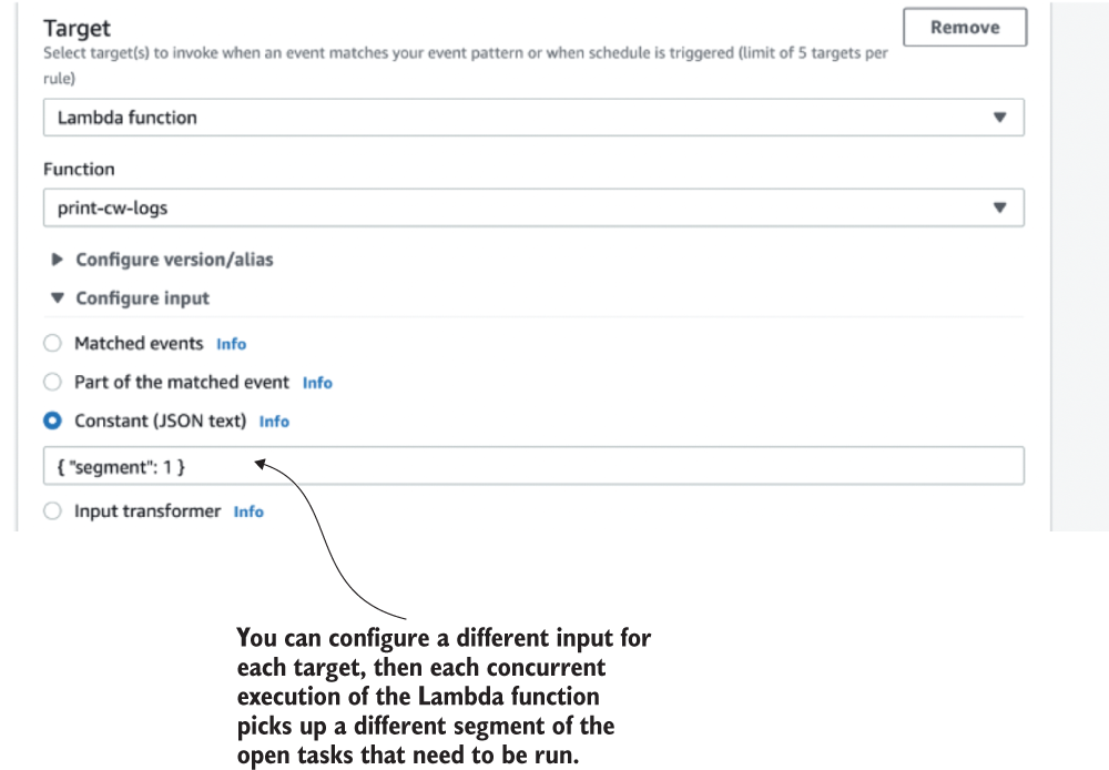
Figure 7.4 You can configure a different input for each target to have them fetch different subsets of scheduled tasks. Then the tasks are not processed multiple times.
7.2.1 Your scores
What do you think of this solution? How would you rate it on a scale of 1 (worst) to 10 (best) against each of the nonfunctional requirements? Write down your scores in the empty spaces in the tables provided for this (see table 7.1 as an example). And remember, there are no right or wrong answers. Just use your best judgement based on the information available.
Table 7.1 Your solution scores for a cron job
7.2.2 Our scores
The biggest advantage of this solution is that it’s really simple to implement. The complexity of a solution is an important consideration in real-world projects because we’re always bound by resource and time constraints. However, for the purpose of this book, we will ignore these real-world constraints and only consider the nonfunctional requirements outlined in section 7.1. With that said, here are our scores for this solution (table 7.2). We’ll then explain our reasons for these scores in the following subsections.
Table 7.2 Our solution scores for a cron job with EventBridge
We gave this solution a 6 for precision because EventBridge cron jobs can run at most once per minute. That’s the best precision we can hope for with this solution. Furthermore, this solution is also constrained by the number of tasks that can be processed in each iteration. When there are too many tasks that need to be run simultaneously, they can stack up and cause delays. These delays are a symptom of the biggest challenge with this solution—dealing with hotspots. More on that next.
Scalability (number of open tasks)
Provided that the open tasks do not cluster together (hotspots), this solution would have no problem scaling to millions and millions of open tasks. Each time the Lambda function runs, it only cares about the tasks that are now overdue. Because of this, we gave this solution a perfect 10 for scalability (number of open tasks).
We gave this solution a lowly 2 for this criteria because a cron job doesn’t handle hotspots well at all. When there are more tasks than the Lambda function can handle in one invocation, this solution runs into all kinds of trouble and forces us into difficult trade-offs.
For example, do we allow the function to run for more than 1 minute? If we don’t, then the function would time out, and there’s a strong possibility that some tasks might be processed but not marked as so because the invocation was interrupted midway through. We need to either make sure the scheduled tasks are idempotent or we have to choose between:
-
Executing some tasks twice if we mark them as processed in the database after successfully processing.
-
Not executing some tasks at all if we mark them as processed in the database before we finish processing them.
-
Employing a mechanism such as the Saga pattern (http://mng.bz/AOEp) for managing the transaction and reliably updating the database record after the task is successfully processed. (This can add a lot of complexity and cost to the solution.)
On the other hand, if we allow the function to run for more than 1 minute, then we are less likely to experience this problem until we see a large enough hotspot that the Lambda function can’t process in 15 minutes! Also, now there can be more than one concurrent execution of this function running at the same time. To avoid the same task being run more than once, we can set the function’s Reserved Concurrency setting to 1. This ensures that at any moment, only one concurrent execution of the Lambda function is running (see figure 7.5). However, this severely limits the potential throughput of the system.

Figure 7.5 If we limit Reserve Concurrency to 1, then there will be only one concurrent execution of the Lambda function running at any moment. This means some cron job cycles will be skipped.
Imagine 1,000,000 tasks that need to be run at 00:00 UTC, but the Lambda function can process only 10,000 tasks per minute. If we do nothing, then the function would timeout, be retried, and would take at least 100 invocations to finish all the tasks. In the meantime, other tasks are also delayed, further exasperating the impact on user experience. This is the Achille’s heel of this solution. But we can tweak the solution to increase its throughput and help it cope with hotspots better. More on this later.
With EventBridge, cron jobs are free, but we have to pay for the Lambda invocations even when there are no tasks to run. You can minimize the Lambda cost if you use a moderate memory size for the cron job. After all, it’s not doing anything CPU-intensive and shouldn’t need a lot of memory (and therefore CPU).
In our scenario, the main cost for this solution is the DynamoDB read and write requests. For every task, you need one write request (when scheduling the task) and one read request (when the cron job retrieves it). This access pattern makes it a good fit for DynamoDB’s on-demand pricing and allows the cost of the solution to grow linearly with its scale. At $1.25 per million write units and $0.25 per million read units, the cost per million scheduled tasks can be as low as $1.50. That’s just the DynamoDB cost, and even that depends on the size of the items you need to store for each task as DynamoDB read/write units are calculated based on payload size. You also have to factor in the Lambda costs too, which also depend on a number of factors such as memory size and execution duration.
Nonetheless, this is still a cost-effective solution, even when you scale to millions of scheduled tasks per day. And, hence, why we gave it a score of 7. Overall, this is a good solution for applications that don’t have to deal with hotspots, and it is also easy to implement. As we mentioned earlier, we can also tweak the architecture slightly to address its problem with hotspots.
7.2.3 Tweaking the solution
Earlier, we mentioned that we can increase the throughput of this solution by allowing multiple concurrent executions of the Lambda to run in parallel. We can do this by duplicating the Lambda function target in the EventBridge rule. Because there’s a limit of five targets per EventBridge rule, we can only hope for a fivefold increase at best. Beyond that, we can also duplicate the EventBridge rule itself as many times as we need.
But even with these tricks, Lambda’s 15 minutes execution time limit is still looming over our head. We also have to shard the reads so that the concurrent executions don’t process the same tasks. Doing that, we also incur higher operational cost and complexity as well. There are more resources to configure and manage, and there are more Lambda invocations and database reads, even though most of the time they’re not necessary. Essentially, we have “provisioned” (for lack of a better term) our application for peak throughput all the time.
Increasing throughput this way is ineffective. A much better alternative is to fan-out the processing logic based on the number of tasks that need to run. Lambda’s burst capacity limit allows up to 3,000 concurrent executions to be created instantly (see https://amzn.to/2BxRuVG). This allows for a huge potential for parallel processing even if we use just a fraction of it. For this to work, we need to move the business logic to fetch and run tasks into another Lambda function. From here, we can invoke as many instances of this new function as we deem necessary when faced with a large batch of tasks (figure 7.6 shows this approach).
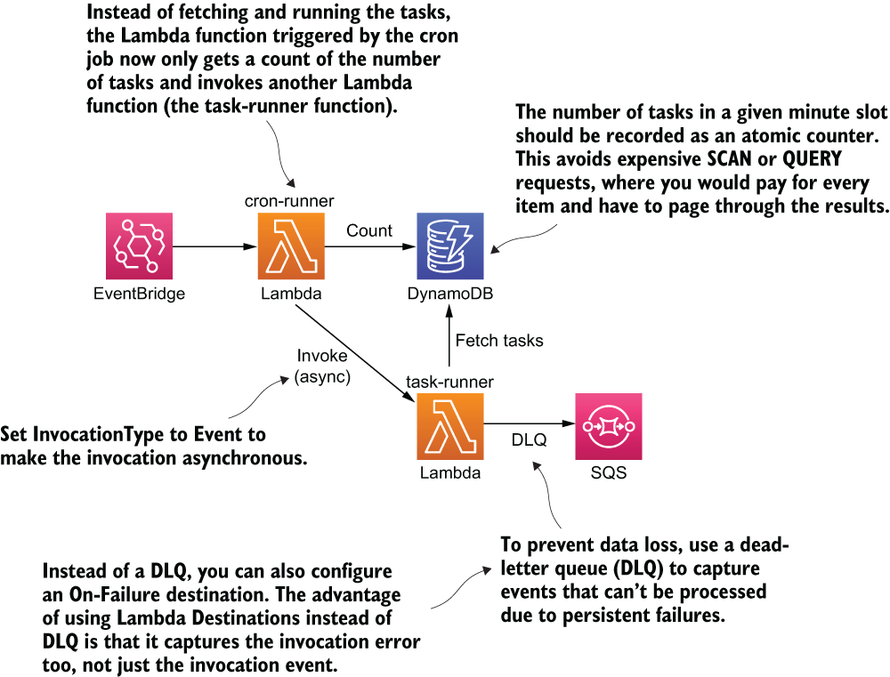
Figure 7.6 An alternative architecture as a solution to our cron job. The solution fans out the processing logic to another function.
Once we know the number of tasks that needs to run, we can calculate the number of concurrent executions we need. To alleviate the time pressure and minimize the danger of timeouts, we can add some headroom into our calculation.
For example, if the throughput for the processing function is 10,000 tasks per minute, then we can start a new concurrent execution for every 5,000 tasks. If there are 1,000,000 tasks, then we need 200 concurrent executions. This is well below the burst capacity limit of 3,000 concurrent executions in the region.
7.2.4 Final thoughts
Cron jobs can be a simple and yet effective solution. As you saw, with some small tweaks it can also be scaled to support even large hotspots. However, it tends to push a lot of the load onto the database. In the aforementioned scenario of 1,000,000 tasks that need to be run in a single minute, it would require 1,000,000 reads from DynamoDB. Luckily for us, DynamoDB can handle this level of traffic, although we need to be careful with the throughput limits that are in place. For example, DynamoDB has a default limit of 40,000 read units per table for on-demand tables (https://amzn.to/3eH0THZ).
What if there’s a way to implement the scheduling service without having to read from the DynamoDB table at all? It turns out we can do that by taking advantage of DynamoDB’s time-to-live (TTL) feature (https://amzn.to/2NRgARU).
7.3 DynamoDB TTL
DynamoDB lets you specify a TTL value on items, and it deletes the items after the TTL has passed. This is a fully managed process, so you don’t have to do anything yourself besides specifying a TTL value for each item.
You can use the TTL value to schedule a task that needs to run at a specific time. When the item is deleted from the table, a REMOVE event is published to the corresponding DynamoDB stream. You can subscribe a Lambda function to this stream and run the task when it’s removed from the table (figure 7.7).

Figure 7.7 High-level architecture using DynamoDB TTL to run ad hoc scheduled tasks.
There are a couple of things to keep in mind about this solution. The first, and most important, is that DynamoDB TTL doesn’t offer any guarantee on how quickly it deletes expired items from the table. In fact, the official documentation (https://amzn.to/2NRgARU) only goes as far as to say, “TTL typically deletes expired items within 48 hours of expiration” (see figure 7.8). In practice, the actual timing is usually not as bleak. Based on empirical data that we collected, items are usually deleted within 30 minutes of expiration. But as figure 7.8 shows, it can vary greatly depending on the size and activity level of the table.

Figure 7.8 DynamoDB TLL’s notification regarding its ability to delete expired items in tables
The second thing to consider is that the throughput of the DynamoDB stream is constrained by the number of shards in the stream. The number of shards is, in turn, determined by the number of partitions in the DynamoDB table. However, there’s no way for you to directly control the number of partitions. It’s entirely managed by DynamoDB, based on the number of items in the table and its read and write throughputs.
We know we’re throwing a lot of information at you about DynamoDB, including some of its internal mechanics such as how it partitions data. Don’t worry if these are all new to you, you can learn a lot about how DynamoDB works under the hood by watching this session from AWS re:invent 2018: https://www.youtube.com/watch?v=yvBR71D0nAQ.
7.3.1 Your scores
What do you think of this solution? How would you rate it on a scale of 1 to 10 for each of the nonfunctional requirements? As before, write your scores in the empty spaces in table 7.3.
Table 7.3 Your scores for DynamoDB TTL
7.3.2 Our scores
The biggest problem with this solution is that DynamoDB TTL does not delete the scheduled items reliably. This limitation means it’s not suitable for any application that is remotely time sensitive. With that said, here are our scores in table 7.4. Again, we present how we arrived at these scores in the following subsections.
Table 7.4 Our scores for DynamoDB TTL
Scheduled tasks would be run within 48 hours of their scheduled time. A score of 1 might be considered a flattering score here.
Scalability (number of open tasks)
We gave this solution a perfect 10 because the number of open tasks equals the number of items in the scheduled_tasks table. Because DynamoDB has no limit on the total number of items you can have in a table, this solution can scale to millions of open tasks. Unlike relational databases, whose performance can degrade quickly as the database gets bigger, DynamoDB offers consistent and fast performance no matter how big it gets. Figure 7.9 provides a testimony to its performance.
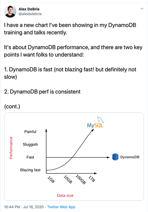
Figure 7.9 A satisfied customer’s statement regarding DynamoDB’s scalability and number of opened tasks
We gave this solution a 6 because it can still face throughput-related problems because it’s constrained by the throughput of the DynamoDB stream. But the tasks would be simply queued up in the stream and would run slightly later than scheduled.
Let’s drill into this throughput constraint some more as that is useful for you to understand. As mentioned previously, the number of shards in the DynamoDB stream is managed by DynamoDB. For every shard the Lambda service would have a dedicated concurrent execution of the execute function. You can read more about how Lambda works with DynamoDB and Kinesis streams in the official documentation at https://amzn.to/2ZIu3Cx.
When a large number of tasks are deleted from DynamoDB at the same time, the REMOVE events are queued in the DynamoDB stream for the execute function to process. These events stay in the stream for up to 24 hours. As long as the execute function is able to eventually catch up, then we won’t lose any data.
Although there is no scalability concern with hotspots per se, we do need to consider the factors that affect the throughput of this solution. Ultimately, these throughput limitations will affect the precision of this solution:
-
How quickly the hotspots are processed depends on how quickly DynamoDB TTL deletes those items. DynamoDB TTL deletes items in batches, and we have no control over how often it runs and how many items are deleted in each batch.
-
How quickly the execute function processes all the tasks in a hotspot is constrained by how many instances of it runs in parallel. Unfortunately, we can’t control the number of partitions in the scheduled_tasks table, which ultimately determines the number of concurrent executions of the execute function. However, we can override the Concurrent Batches Per Shard configuration setting (https://amzn.to/2YUGE59), which allows us to increase the parallelism factor tenfold (see figure 7.10).

Figure 7.10 You can find the Concurrent Batches Per Shard setting under Additional Settings for Kinesis and DynamoDB Stream functions.
This solution requires no DynamoDB reads. The deleted item is included in the REMOVE events in the DynamoDB stream. Because events in the DynamoDB stream are received in batches, they are efficient to process and require fewer Lambda invocations. Furthermore, DynamoDB Streams are usually charged by the number of read requests, but it’s free when you process events with Lambda. Because of these characteristics, this solution is extremely cost effective even when it’s scaled to many millions of scheduled tasks. Hence, this is why we gave it a perfect 10 for Cost.
7.3.3 Final thoughts
This solution makes creative use of the TTL feature in DynamoDB and gives you an extremely cost-effective solution for running scheduled tasks. However, because DynamoDB TTL doesn’t offer any reasonable guarantee on how quickly tasks are deleted, it’s ill-fitted for many applications. In fact, neither cron jobs nor DynamoDB TTL are well-suited for applications where tasks need to be run within a few seconds of their scheduled time. For these applications, our next solution might be the best fit as it offers unparalleled precision at the expense of other nonfunctional requirements.
7.4 Step Functions
Step Functions is an orchestration service that lets you model complex workflows as state machines. It can invoke Lambda functions or integrate directly with other AWS services such as DynamoDB, SNS, and SQS when the state machine transitions to a new state.
One of the understated superpowers of Step Functions is the Wait state (https://amzn.to/38po884). It lets you pause a workflow for up to an entire year! Normally, idle waiting is difficult to do with Lambda. But with Step Functions, it’s as easy as a few lines of JSON:
"wait_ten_seconds": {
  "Type": "Wait",
  "Seconds": 10,
  "Next": "NextState"
}
You can also wait until a specific UTC timestamp:
"wait_until": {
  "Type": "Wait",
  "Timestamp": "2016-03-14T01:59:00Z",
  "Next": "NextState"
}
And using TimestampPath, you can parameterize the Timestamp value using data that is passed into the execution:
"wait_until": {
  "Type": "Wait",
  "TimestampPath": "$.scheduledTime",
  "Next": "NextState"
}
To schedule an ad hoc task, you can start a state machine execution and use a Wait state to pause the workflow until the specified date and time. This solution is precise. Based on the data we have collected, tasks are run within 0.01 second of the scheduled time in the 90th percentile. However, there are several service limits to keep in mind (see https://amzn.to/2C4fGPD):
-
There are limits to the StartExecution API. This API limits the rate at which you can schedule new tasks because every task has its own state machine execution (see figure 7.11).

Figure 7.11 StartExecution API limit for AWS Step Functions
-
There are limits to the number of state transitions per second. When the Wait state expires, the scheduled task runs. However, when there are large hotspots where many tasks all run simultaneously, these can be throttled because of this limitation (see figure 7.12).

Figure 7.12 State transition limit for AWS Step Functions
-
There is a default limit of 1,000,000 open executions. Because there is one open execution per scheduled task, this is the maximum number of open tasks the system can support.
Thankfully, all of these limits are soft limits, which means you can increase them with a service limit raise. However, given that the default limits for some of these are pretty low, it might not be possible to raise to a level that can support running a million scheduled tasks in a single hotspot.
There is also the hard limit on how long an execution can run, which is one year. This limits the system to schedule tasks that are no further than a year away. For most use cases, this would likely be sufficient. If not, we can tweak the solution to support tasks that are scheduled for more than a year away (more on this later).
7.4.1 Your scores
What do you think of this solution? How would you rate it on a scale of 1 to 10 against each of the nonfunctional requirements? As before, write down your scores in the empty spaces provided by table 7.5.
Table 7.5 Your solution scores for Step Functions
7.4.2 Our scores
Step Functions gives us a simple and elegant solution for the problem at hand. However, it’s hampered by several service limits that makes it difficult to scale. We will dive into these limitations, but first, table 7.6 shows our scores for this solution.
Table 7.6 Our scores for Step Functions
As we mentioned before, Step Functions is able to run tasks within 0.01 s precision at the 90th percentile. It just doesn’t get more precise than that!
Scalability (number of open tasks)
We gave this solution a 7 because the StartExecution API limit restricts how many scheduled tasks we can create per second. Whereas solutions that store scheduled tasks in DynamoDB can easily scale to scheduling tens of thousands of tasks per second, here we have to contend with a default refill rate of just 300 per second in the larger AWS regions. Luckily, it is a soft limit, so technically we can raise it to whatever we need. But the onus is on us to constantly monitor its usage against the current limit to prevent us from being throttled.
The same applies to the limit on the number of open executions. While the default limit of 1,000,000 is generous, we still need to keep an eye on the usage level. Once we reach the limit, no new tasks can be scheduled until existing tasks are run. User behavior would have a big impact here. The more uniformly the tasks are distributed over time, the less likely this limit would be an issue.
We gave this solution a 4 because the limit on StateTransition per second is problematic if a large cluster of tasks needs to run during the same time. Because the limit applies to all state transitions, even the initial Wait states could be throttled and affect our ability to schedule new tasks.
We can increase both the bucket size (think of it as the burst limit) as well as the refill rate per second. But raising these limits alone might not be enough to scale this solution to support large hotspots with, say, 1,000,000 tasks. Thankfully, there are tweaks we can make to this solution to help it handle large hotspots better, but we need to trade off some precision (more on this later).
We gave this solution a 2 because Step Functions is one of the most expensive services on AWS. We are charged based on the number of state transitions. For a state machine that waits until the scheduled time and runs the task, there are four states (see figure 7.13), and every execution charges for these state transitions (http://mng.bz/ZxGm).

Figure 7.13 A simple state machine that waits until the scheduled time to run its task
At $0.025 per 1,000 state transitions, the cost for scheduling 1,000,000 tasks would be $100 plus the Lambda cost associated with executing the tasks. This is nearly two orders of magnitude higher than the other solutions considered so far.
7.4.3 Tweaking the solution
So far, we have discussed several problems with this solution: not being able to schedule tasks for more than a year and having trouble with hotspots. Fortunately, there are simple modifications we can make to address these problems.
Extend the scheduled time beyond one year
The maximum time a state machine execution can run for is one year. As such, the maximum amount of time a Wait state can wait for is also one year. However, we can extend this limitation by borrowing the idea of tail recursion (https://www.geeksforgeeks.org/tail-recursion/) from functional programming. Essentially, at the end of a Wait state, we can check if we need to wait for even more time. If so, the state machine starts another execution of itself and waits for another year, and so on. Until eventually, we arrive at the task’s scheduled time and run the task.
This is similar to a tail recursion because the first execution does not need to wait for the recursion to finish. It simply starts the second execution and then proceeds to complete itself. See figure 7.14 for how this revised state machine might look.
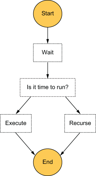
Figure 7.14 A revised state machine design that can support scheduled tasks that are more than one year away
Sometimes, just raising the soft limits on the number of StateTransitions per second alone is not going to be enough. Because the default limits have a bucket size of 5,000 (the initial burst limit) and a refill rate of 1,500 per second, if we are to support running 1,000,000 tasks around the same time, we will need to raise these limits by multiple orders of magnitude. AWS will be unlikely to oblige such a request, and we will be politely reminded that Step Functions is not designed for such use cases.
Fortunately, we can make small tweaks to the solution to make it far more scalable when it comes to dealing with hotspots. Unfortunately, we will need to trade off some of the precision of this solution for the new found scalability.
For example, instead of running every task scheduled for 00:00 UTC at exactly 00:00 UTC, we can spread them across a 1-minute window. We can do this by adding some random delay to the scheduled time. Following this simple change, some of the aforementioned tasks would be run at 00:00:12 UTC, and some would be run at 00:00:47 UTC, for instance. This allows us to make the most of the available throughput. With the default limit of 5,000 bucket size and refill rate of 1,500 per second, the maximum number of state transitions per minute is 93,500:
Doing this would reduce the precision to “run within a minute,” but we wouldn’t need to raise the default limits by nearly as much. It’ll be a trivial change to inject a variable amount of delay (0-59 s) to the scheduled time so that tasks are uniformly distributed across the minute window. With this simple tweak, Step Functions is no longer the scalability bottleneck. Instead, we will need to worry about the rate limits on the Lambda function that will run the task.
Another alternative would be to have each state machine execution run all the tasks that are scheduled for the same minute in batches and in parallel. For example, when scheduling a task, add the task with the scheduled time in a DynamoDB table as the HASH key and a unique task ID as the RANGE key. At the same time, atomically increment a counter for the number of tasks scheduled for this timestamp. Both of these updates can be performed in a single DynamoDB transaction. Figure 7.15 shows how the table might look.

Figure 7.15 Set the scheduled task as well as the count in the same DynamoDB table.
We would start a state machine execution with the timestamp as the execution name. Because execution names have to be unique, the StartExecution request will fail if there’s an existing execution already. This ensures that only one execution is responsible for running all the tasks scheduled for that minute (2020-07-04T21:53:22).
Instead of executing the scheduled tasks immediately after the Wait state, we could get a count of the number of tasks that need to run. From here, we would use a Map state to dynamically generate parallel branches to run these tasks in parallel. See figure 7.16 for how this alternative design might look.

Figure 7.16 An alternative design for the state machine that can run tasks in batches in parallel
Making these changes would not affect the precision by too much, but it would reduce the number of state machine executions and Lambda invocations required. Essentially, we would need one state machine execution for every minute when we need to run some scheduled tasks. There is a total of 525,600 minutes in a 365 days calendar year, so this also removes the need to increase the limit on the number of open executions (again, the default limit is 1,000,000). That’s the beauty of these composable architecture components! Because there are so many ways to compose them, it gives you lots of different options and trade-offs.
7.4.4 Final thoughts
Step Functions offers a simple and elegant solution that can run tasks at great precision. The big drawback are its costs and the various service limits that you need to look out for, which hampers its scalability. But as you can see, if we are willing to make tradeoffs against precision, we can modify the solution to make it much more scalable.
We looked at a couple of possible modifications, including taking some elements of the cron job solution and turning this solution into a more flexible cron job that only runs when there are tasks that need to run. We also looked at a modification that allows us to work around the 1-year limit by applying tail recursion to the state machine design. In the next solution, we’ll apply the same technique to SQS as it is bound by an even tighter constraint on how long a task can stay open.
7.5 SQS
The Amazon Simple Queue Service (SQS) is a fully managed queuing service. You can send messages to and receive messages from the queue. Once a message has been received by a consumer, the message is then hidden from all other consumers for a period of time, which is known as the visibility timeout. You can configure the visibility timeout value on the queue, but the setting can also be overridden for individual messages.
When you send a message to SQS, you can also use the DelaySeconds attribute to make the message become visible at the right time. You can implement the scheduling service by using these two settings to hide a message until its scheduled time. However, the maximum DelaySeconds is a measly 15 minutes, and the maximum visibility timeout is only 12 hours. But all is not lost.
When the execute function receives the message after the initial DelaySeconds, it can inspect the message and see if it’s time to run the task (see figure 7.17). If not, it can call ChangeMessageVisibility on the message to hide the message for up to another 12 hours (https://amzn.to/3e1GVY6). It can do this repeatedly until it’s finally time to run the scheduled task.
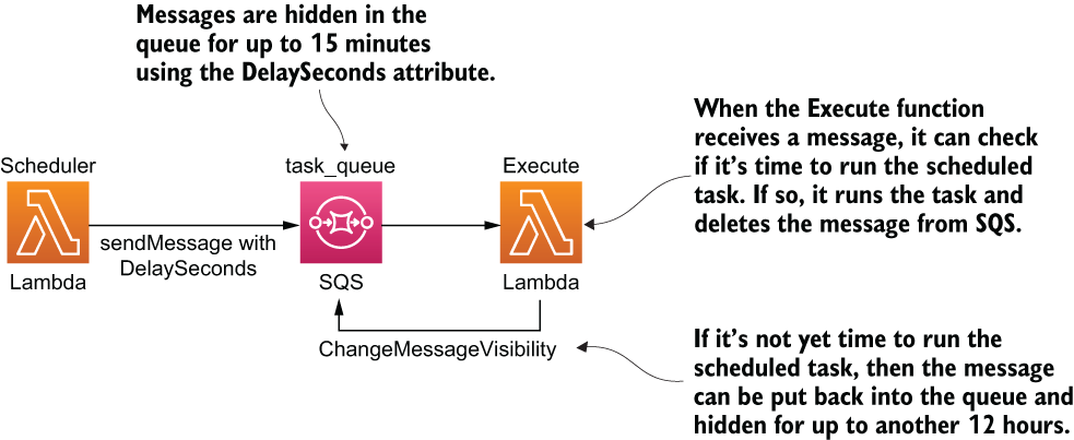
Figure 7.17 High-level architecture of using SQS to schedule ad hoc tasks
Before you score this solution, consider that there is a limit of 120,000 inflight messages. Unfortunately, this is a hard limit and cannot be raised. This limit has a profound implication that can mean it’s not suitable for some use cases at all!
Once a message is inflight, this solution would keep it inflight by continuously extending its visibility timeout until its scheduled time. In this case, the number of inflight messages equates to the number of open tasks. However, once you reach the 120,000 inflight messages limit, then newer messages would stay in the queue’s backlog, even if some of the newer messages might need to run sooner than the messages that are already inflight. Priority is given to tasks based on when they were scheduled, not by their execution time.
This is not a desirable characteristic for a scheduling service. In fact, it’s the opposite of what we want. Tasks that are scheduled to execute soon should be given the priority to ensure they’re executed on time. That being said, this is a problem that would only arise when you have reached the 120,000 inflight messages limit. The further away tasks can be scheduled, the more open tasks you would have, and the more likely you would run into this problem.
7.5.1 Your scores
With this severe limitation in mind, how would you score this solution? Write down your scores in the empty spaces in table 7.7.
Table 7.7 Your solution scores for SQS
7.5.2 Our scores
This solution is best suited for scenarios where tasks are not scheduled too far away in time. Otherwise, we face the prospect of accumulating a large number of open tasks and running into the limit on inflight messages. Also, we would need to call ChangeMessageVisibility on the message every 12 hours for a long time. If a task is scheduled to execute in a year, then that’s a total of 730 times. Multiplied that by 1,000,000 tasks and that’s a total of 730 million API requests or $292 for keeping 1,000,000 tasks open for a whole year. With these in mind, table 7.8 shows our scores.
Table 7.8 Our solution scores for SQS
Under normal conditions, SQS messages that are delayed or hidden are run no more than a few seconds after their scheduled times. Not as precise as Step Functions, but still very good. This is why we gave this solution a score of 9.
Scalability (number of open tasks)
We gave this solution a low score because the hard limit of 120,000 inflight messages severely limits this solution’s ability to support a large number of open tasks. Even though the tasks can still be scheduled, they cannot run until the number of inflight messages drops below 120,000. This is a serious hinderance and, in the worst cases, can render the system completely unusable. For example, if 120,000 tasks are scheduled to run in one year, then nothing else that’s scheduled after that can run until those first 120,000 tasks have been run.
The Lambda service uses long polling to poll SQS queues and only invokes our function when there are messages (http://mng.bz/Rqyj). These pollers are an invisible layer between SQS and our function, and we do not pay for them. But we do pay for the SQS ReceiveMessage requests they make. According to this blog post by Randall Hunt (https://amzn.to/31MfVtl)
The Lambda service monitors the number of inflight messages, and when it detects that this number is trending up, it will increase the polling frequency by 20 ReceiveMessage requests per minute and the function concurrency by 60 calls per minute. As long as the queue remains busy it will continue to scale until it hits the function concurrency limits. As the number of inflight messages trends down Lambda will reduce the polling frequency by 10 ReceiveMessage requests per minute and decrease the concurrency used to invoke our function by 30 calls per-minute.
By keeping the queue artificially busy with a high number of inflight messages, we are artificially raising Lambda’s polling frequency and function concurrency. This is useful for dealing with hotspots.
Because of the way this solution works, all open tasks are kept as inflight messages. This means the Lambda service would likely be running a high number of concurrent pollers all the time. When a cluster of messages become available at the same time, they will likely be processed by the execute function with a high degree of parallelism. And Lambda scales up the number of concurrent executions as more messages become available. We can, therefore, use the autoscaling capability that Lambda offers.
Because of this, we gave this solution a really good score. But, on the other hand, this behavior generates a lot of redundant SQS ReceiveMessage requests, which can have a noticeable impact on cost when running at scale.
Between the many ReceiveMessage requests Lambda makes on our behalf and the cost of calling ChangeMessageVisibility on every message every 12 hours, most of the cost for this solution will likely be attributed to SQS. While SQS is not an expensive service, at $0.40 per million API requests, the cost can accumulate quickly because this solution is capable of generating many millions of requests at scale. As such, we gave this solution a 5, which is to say that it’s not great but also unlikely to cause you too much trouble.
7.5.3 Final thoughts
If you put the scores for this solution side-by-side with DynamoDB TTL, you can see that they perfectly complement each other. Where one is strong, the other is weak. Table 7.9 shows the ratings for both services.
Table 7.9 Our ratings for SQS vs. DynamoDB TTL
What if we can combine these two solutions to create a solution that offers the best of both worlds? Let’s look at that next.
7.6 Combining DynamoDB TTL with SQS
So far, we have seen that the DynamoDB TTL solution is great at dealing with a large number of open tasks, but lacks the precision required for most use cases. Conversely, the SQS solution is great at providing good precision and dealing with hotspots but can’t handle a large number of open tasks. The two rather complement each other and can be combined to great effect.
For example, what if long-term tasks are stored in DynamoDB until two days before their scheduled time? Why two days? Because it’s the only soft guarantee that DynamoDB TTL gives:
TTL typically deletes expired items within 48 hours of expiration (https://amzn.to/ 2NRgARU).
Once the tasks are deleted from the DynamoDB table, they are moved to SQS where they are kept inflight until the scheduled time (using the ChangeMessageVisibility API as discussed earlier). For tasks that are scheduled to execute in less than two days, they are added to the SQS queue straight away. See figure 7.18 for how this solution might look.

Figure 7.18 High-level architecture of combining DynamoDB TTL with SQS
7.6.1 Your scores
How would you score this solution? Again, write your scores in the empty spaces in table 7.10.
Table 7.10 Your solution scores for DynamoDB TTL with SQS
7.6.2 Our scores
According to “The Fundamental theorem of software engineering” (https://dzone.com/articles/why-fundamental-theorem):
We can solve any problem by introducing an extra level of indirection.
Like the other alternative solutions we saw earlier in this chapter, this solution solves the problems with an existing solution by introducing an extra level of indirection. It does so by composing different services together in order to make up for the shortcomings of each. Take a look at table 7.11 for our scores for this solution, then we’ll discuss how we arrived at these scores.
Table 7.11 Our solution scores for DynamoDB TTL with SQS
As all the executions go through SQS, this solution has the same level of precision as the SQS-only solution, 9.
Scalability (number of open tasks)
Storing long-term tasks in DynamoDB largely solves SQS’s problem with scaling the number of open tasks. However, it is still possible to run into the 120,000 inflight messages limit with just the short-term tasks. It’s far less likely, but it is still a possibility that needs to be considered. Hence, we marked this solution as an 8.
As all the executions go through SQS, this solution has the same score as the SQS-only solution, 8.
This solution eliminates most of the ChangeMessageVisibility requests because all the long-term tasks are stored in DynamoDB. This cuts out a large chunk of the cost associated with the SQS solution. However, in return, it adds additional costs for DynamoDB usage and Lambda invocations for the reschedule function. Overall, the costs this solution takes away are greater than the new costs it adds. Hence, we gave it a 7, improving on the original score of 5 for the SQS solution.
7.6.3 Final thoughts
This is just one example of how different solutions or aspects of them can be combined to make a more effective answer. This combinatory effect is one of the things that makes cloud architectures so interesting and fascinating, but also, so complex and confusing at times. There are so many different ways to achieve the same goal, and depending on what your application needs, there’s usually no one-size-fits-all solution that offers the best results for all applications.
So far, we have only looked at the supply side of the equation and what each solution can offer. We haven’t looked at the demand side yet or what application needs what. After all, depending on the application, you might put a different weight behind each of the nonfunctional requirements. Let’s try to match our solutions to the right application next.
7.7 Choosing the right solution for your application
Table 7.12 shows our scores for the five solutions that we considered in this chapter. The solutions in this table do not include the proposed tweaks. Depending on the application, some of these requirements might be more important than others.
Table 7.12 Our scores for all five solutions
7.8 The applications
Let’s consider three applications that might use the ad hoc scheduling service:
-
Application 2 is a multi-player app for a mobile game, which we’ll call TournamentsRUs.
-
Application 3 is a healthcare app that digitizes and manages your consent for sharing your medical data with care providers, which we’ll call iConsent.
In the reminder app, RemindMe, users can create reminders for future events, and the system will send SMS/push notifications to the users 10 minutes before the event. While reminders are usually distributed evenly over time, there are hotspots around public holidays and major sporting events such as the Super Bowl. During these hotspots, the application might need to notify millions of users. Fortunately, because the reminders are sent 10 minutes before the event, the system gives us some slack in terms of timing.
In application 2, the multi-player mobile app called TournamentsRUs, players compete in user-generated tournaments that are 15-30 minutes long. As soon as the final whistle blows, the tournament ends and all participants wait for a winner to be announced via an in-game popup. TournamentsRUs currently has 1.5 million daily active users (DAU) and hopes to double that number in 12 months’ time. At peak, the number of concurrent users is around 5% of its DAU, and tournaments typically consist of 10-15 players each.
In application 3, the healthcare app iConsent, users fill in digital forms that allow care providers to access their medical data. Each consent has an expiration date, and the app needs to change its status to expired when the expiration date passes. iConsent currently has millions of registered users, and users have an average of three consents.
Each of these applications need to use a scheduling service to run ad hoc tasks at specific times, but their use cases are drastically different. Some deal with tasks that are short-lived, while others allow tasks to be scheduled for any future point in time. Some are prone to hotspots around real-world events; others can accumulate large numbers of open tasks because there is no limit to how far away tasks can be scheduled.
To help us better understand which solution is the best for each application, we can apply a weight against each of the nonfunctional requirements. For example, TournamentsRUs cares a lot about precision because users will be waiting for their results at the end of a tournament. If the tasks to finalize tournaments are delayed, then it can negatively impact the users’ experience with the app.
7.8.1 Your weights
For each of the applications, write a weight between 1 (“I don’t care”) and 10 (“This is critical”) for each of the nonfunctional requirements in table 7.13. Remember, there are no right or wrong answers here! Use your best judgement based on the limited amount of information you know about each app.
Table 7.13 Your ratings for RemindMe, TournamentsRUs, and iConsent
7.8.2 Our weights
Table 7.14 shows our weightings. Are these scores similar to yours? We’ll go through each application and talk about how we arrived at these weights in the sections following the table.
Table 7.14 Our scores for RemindMe, TournamentsRUs, and iConsent
We gave Precision a weight of 5 for this app because reminders are sent 10 minutes before the event. This gives us a lot of slack. Even if the reminder is sent 5 minutes late, it’s still OK.
Scalability (number of open tasks) gets a weight of 10 because there are no upper bounds on how far out the events can be scheduled. At any moment, there can be millions of open reminders. This makes scaling the number of open tasks an absolutely critical requirement for this application. For Scalability (hotspots), we gave a weight of 8 because large hotspots would likely form around public holidays (for example, mother’s day) and sporting events (for example, the Super Bowl or the Olympics).
Finally, for Cost, we gave it a weight of 3. This perhaps reflects our general attitude towards the cost of serverless technologies. Their pay-per-use pricing allows our cost to grow linearly when scaling. Generally speaking, we don’t want to optimize for cost unless the solution is going to burn down the house!
For TournamentsRUs, Precision gets a weight of 10 because when a tournament finishes, players will all be waiting for the announcement of the winner. If the scheduled task (to finalize the tournament and calculate the winner) is delayed for even a few seconds, it would provide a bad user experience.
We gave Scalability (number of open tasks) a weight of 6 because only a small percentage of its DAUs are online at once and because of the short duration of its tournaments. At 1.5 M DAU, 5% concurrent users at peak and an average of 10-15 players in each tournament, these numbers translate to approximately 5,000-7,500 open tournaments during peak times.
For Scalability (hotspots), it received a lowly 3 because the tournaments are user-generated and have different lengths of time (between 15-30 minutes). It’s unlikely for large hotspots to form under these conditions. And, as with RemindMe, we gave Cost a weight of 3 (just don’t burn my house down!).
Lastly, for iConsent, Precision received a weight of 4. When a consent expires, it should be shown in the UI with the correct status. However, because the user is probably not going to check the app every few minutes for updates, it’s OK if the status is updated a few minutes (or maybe even an hour) later.
We gave a weight of 10 for Scalability (number of open tasks). This is because medical consents can be valid for a year or sometimes even longer: all of these active consents are open tasks, so the system would have millions of open tasks at any moment. For Scalability (hotspots) on the other hand, we gave it a weight of 1 because there is just no natural clustering that can lead to hotspots. And finally, cost gets a weight of 3 because that’s just how we generally feel about cost for serverless applications.
7.8.3 Scoring the solutions for each application
So far, we have scored each solution based on its own merits. But this says nothing about how well suited a solution is to an application because, as we have seen, applications have different requirements. By combining a solution’s scores with an application’s weights, we can arrive at something of an indicative score of how well they are suited for each other. Let’s show you how this can be done and then you can do this exercise yourself. If you recall, the following table shows our scores for the cron job solution:
For RemindMe, we gave the following weights:
Now, if we multiple the score with the weight for each nonfunctional requirement, we will arrive at the scores in the following table:
This adds up to a grand total of 30 + 100 + 16 + 21 = 167. On its own, this score means very little. But if we repeat the exercise and score each of the solutions for RemindMe, then we can see how well they compare with each other. This would help us pick the most appropriate solution for RemindMe, which might be different than the solution you would use for TournamentsRUs or iConsent.
With that in mind, use the whitespace in table 7.15 to calculate your weighted scores for each of the five solutions that we have discussed so far for RemindMe. Then do the same for TournamentsRUs and IConsent in tables 7.16 and 7.17, respectively.
Table 7.15 Weighted scores for the app RemindMe
Table 7.16 Weighted scores for the app TournamentsRUs
Table 7.17 Weighted scores for the app iConsent
Did the scores align with your gut instinct for which solution is best for each application? Did you find something unexpected in the process? Did some solutions not fare as well as you thought they might?
If you find any uncomfortable outcomes as a result of these exercises, then they have done their job. The purpose of defining requirements up front and putting a weight against each requirement is to help us remain objective and combat cognitive biases. Table 7.18 shows our total weighted scores for each solution and application.
Table 7.18 Our total weighted scores for RemindMe, TournamentsRUs, and iConsent
These scores give you a sense as to which solutions are best suited for each application. But they don’t give you definitive answers and you shouldn’t follow them blindly. For instance, there are often factors that aren’t included in the scoring scheme but need to be taken into account nonetheless. Factors such as complexity, resource constraints, and familiarity with the technologies are usually important for real-world projects.
Summary
In this chapter, we analyzed five different ways to implement a service for executing ad hoc tasks, and we judged these solutions on the nonfunctional requirements we set out at the start of the chapter. Throughout the chapter we asked you to think critically about how well each solution would perform for these nonfunctional requirements and asked you to rate them. And we shared our scores with you and our rationale for these scores. We hope through these exercises you have gained some insights into how we approach problem solving and the considerations that goes into evaluating a potential solution:
-
What are the relevant service limits and how do they affect the scalability requirements of the application?
-
What are the performance characteristics of the services in question and do they match up with the application’s needs?
-
How are the services charged? Project the cost of the application by thinking through how the application would need to use these AWS services and applying the services’ billing model to that usage pattern.
These points are a lot easier said than done and it takes practice to become proficient at them. The AWS services are always evolving and new services and features become available all the time so you also have to continuously educate yourself as new options and techniques emerge. Despite having worked with AWS for over a decade, we are still learning ourselves and having to constantly update our own understanding of how different AWS services operate.
Furthermore, AWS do not publish the performance characteristics for many of its services. For example, how soon does Step Functions execute a Wait state after the specific timestamp. If your solution depends on assumptions about these unknown performance characteristics, then you should design small experiments to test your assumptions. In the course of writing this chapter, we conducted several experiments to find out how soon Step Functions and SQS executes delayed tasks. Failing to validate these assumptions early can have devastating consequences. Months of engineering work might go to waste if an entire solution was built on false assumptions.
At the end of the chapter we also asked you to do an exercise of finding the best solution for a given problem and gave you three example applications, each with a different set of needs. The scoring method we asked you to apply is not fool-proof but helps you make objective decisions and combat confirmation biases.
As you brainstormed and evaluated the solutions that have been put in front of you in this chapter, I hope you picked up on the even more important lessons here: that all architecture decisions have inherit tradeoffs and not all application requirements are created equally. The fact that different applications care about the characteristics of its architecture to different degrees gives us a lot of room to make smart tradeoffs.
There are so many different AWS services to choose from, each offering a different set of characteristics and tradeoffs. When you use different services together, they can often create interesting synergies. All of these give us a wealth of options to mix and match different architectural approaches and to engage in a creative problem-solving process, and that’s beautiful!