Chapter 8

Simulating Data from Basic Multivariate Distributions

Contents

8.1 Overview of Simulation from Multivariate Distributions

In the classic reference book, Random Number Generation and Monte Carlo Methods, the author writes, “Only a few of the standard univariate distributions have standard multivariate extensions” (Gentle 2003, p. 203). Nevertheless, simulating data from multivariate data is an important technique for statistical programmers.

If you have p uncorrelated variables, then you can independently simulate each variable by using techniques from the previous chapters. However, the situation becomes more complicated when you need to simulate p variables with a prescribed correlation structure.

This chapter describes how to simulate data from some well-known multivariate distributions, including the multinomial and multivariate normal (MVN) distributions.

8.2 The Multinomial Distribution

There has been considerable research on simulating data from various continuous multivariate distributions. In contrast, there has been less research devoted to simulating data from discrete multivariate distributions. With the exception of the multinomial distribution, some reference books do not mention multivariate discrete distributions at all.

This section describes how to generate random samples from the multinomial distribution. Chapter 9, “Advanced Simulation of Multivariate Data,” describes how to simulate correlated binary variates and correlated ordinal variates.

The multinomial distribution is related to the “Table” distribution, which is described in Section 2.4.5. Suppose there are k items in a drawer and p_i is the probability of drawing item i, i = 1,…, k, where Σ_i p_i = 1. If you draw N items with replacement, then the number of items chosen for each item makes a single draw from the multinomial distribution. For example, in Section 2.4.5, 100 socks were drawn (with replacement) from a drawer with three colors of socks. A draw might result in 48 black socks, 21 brown socks, and 31 white socks. That triplet of values, (48, 21, 31), is a single observation for the multinomial distribution of three categories (the colors) with the given probabilities.

Notice that if there are only two categories with selection probabilities p and 1 – p, then the multinomial distribution is equivalent to the binomial distribution with parameter p.

You can sample from the multinomial distribution in SAS/IML software by using the RANDMULTINOMIAL function. The RANDMULTINOMIAL function computes a random sample by using the conditional distribution technique that is described in Section 8.7.1. The syntax of the RANDMULTINOMIAL function is

X = RandMultinomial(NumSamples, NumTrials, Prob);

where NumSamples is the number of observations in the sample, NumTrials is the number of independent draws of the k categories, and Prob is a 1 × k vector of probabilities that sum to 1.

The following statements generate a 1000 × 3 matrix, where each row is a random observation from a multinomial distribution. The parameters used here are the same parameters that were used in Section 2.4.5. The first five random draws are shown in Figure 8.1.

%let N = 1000;              /* size of each sample */
proc iml;
call randseed(4321);        /* set seed for RandMultinomial */
prob = {0.5 0.2 0.3};
X = RandMultinomial(&N, 100, prob);    /* one sample, N × 3 matrix */

/* print a few results */
c = {“black”, “brown”, “white”};
first = X[1:5,];
print first[colname=c label=“First 5 Obs: Multinomial”];

Figure 8.1 Random Draws from Multinomial Distribution

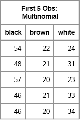
Notice that the sum across each row is 100 because each row is the frequency distribution that results from drawing 100 socks (with replacement). Although there is variation within each column, elements in the first column are usually close to the expected value of 50, elements in the second column are close to 20, and elements in the third column are close to 30. You can examine the distribution of each component of the multivariate distribution by computing the column means and standard deviations, as shown in Figure 8.2:

mean = mean(X);
std = std(X);
corr = corr(X);
print mean[colname=c],
      std[colname=c],
      corr[colname=c rowname=c format=BEST5.];

Figure 8.2 Descriptive Statistics of Components of Multinomial Variables

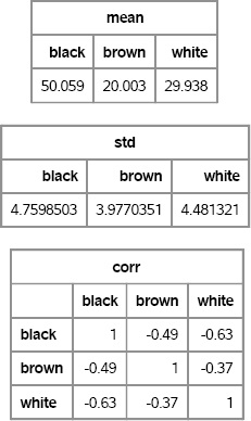
Figure 8.2 shows that the variables are negatively correlated with each other. This makes sense: There are exactly 100 items in each draw, so if you draw more of one color, you will have fewer of the other colors. In fact, the correlation of the component random variables X_i and X_j is .

You can visualize the multinomial distribution by plotting the first two components against each other, as shown in Figure 8.3. (The third component is always 100 minus the sum of the first two components, so you do not need to plot it.) The multinomial distribution is a discrete distribution whose values are counts, so there is considerable overplotting in a scatter plot of the components. One way to resolve the overplotting is to overlay a kernel density estimate. Areas of high density correspond to areas where there are many overlapping points.

/* write multinomial data to SAS data set */
create MN from X[c=c]; append from X; close MN;
quit;

ods graphics on;
proc kde data=MN;
   bivar black brown / plots=ContourScatter;
run;

Figure 8.3 Density Plot of Multinomial Components

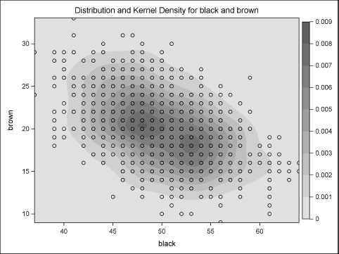
Figure 8.3 shows the negative correlation in the simulated data. It also shows that most of the density is near the population mean (50, 20), although some observations are far from the mean.

Exercise 8.1: A technique that is used to visualize scatter plots that suffer from overplotting is to jitter the values by a small amount. Write a DATA step that adds a uniform random value in [–1/2, 1/2] to each component of the multinomial data. Repeat the call to PROC KDE or use PROC SGPLOT to visualize the jittered distribution.

8.3 Multivariate Normal Distributions

Computationally, the multivariate normal distribution is one of the easiest continuous multivariate distributions to simulate. In SAS software, you can simulate MVN data by using the RANDNORMAL function in SAS/IML software or by using PROC SIMNORMAL, which is in SAS/STAT software. In both cases, you need to provide the mean and covariance matrix of the distribution. If, instead, you have a correlation matrix and a set of variances, then you can use the technique in Section 10.2 to create the corresponding covariance matrix.

The MVN distribution is often a “baseline model in Monte Carlo simulations” (Johnson 1987, p. 55) in the sense that many statistical methods perform well on normal data. You can generate results from normal data and compare them with results from nonnormal data.

In the following sections, MVN data are simulated in two ways:

• The RANDNORMAL function in SAS/IML software. Use this technique when you intend to do additional simulation and analysis in PROC IML. For example, in Chapter 11, “Simulating Data for Basic Regression Models,” the RANDNORMAL function is used as part of simulation to generate data for a mixed model with correlated random effects. In Section 9.2 and Section 9.3, multivariate normal variates are generated as part of a larger algorithm to generate multivariate binary and ordinal data, respectively.
• The SIMNORMAL function in SAS/STAT software. Use this technique when you need to quickly generate data as input for a prewritten macro or procedure.

You might ask whether it is possible to simulate MVN data by using the DATA step. Yes, it is possible, but it is more complicated than using the SAS/IML language because you have to manually implement matrix multiplication in the DATA step. As shown in Fan et al. (2002, Ch. 4), you can use PROC FACTOR to decompose a correlation matrix into a “factor pattern matrix.” You can use this factor pattern matrix to transform uncorrelated random normal variables into multivariate normal variables with the given correlation. Fan et al. (2002) provide a SAS macro to do this. However, calling PROC SIMNORMAL is much easier.

8.3.1 Simulating Multivariate Normal Data in SAS/IML Software

The RANDNORMAL function is available in SAS/IML software; it is not supported by the DATA step. The syntax of the RANDNORMAL function is

X = RandNormal(NumSamples, Mean, Cov);

where NumSamples is the number of observations in the sample, Mean is a 1 × p vector, and Cov is a p × p positive definite matrix. (See Section 10.4 for ways to specify a covariance matrix.) The function returns a matrix, X, where each row is a random observation from the MVN distribution with the specified mean and covariance.

The following statements simulate 1,000 observations from a trivariate normal distribution. Figure 8.4 displays the first few observations of the simulated data, and the sample mean and covariance.

%let N = 1000;                   /* size of each sample */

/* Multivariate normal data */
proc iml;
/* specify the mean and covariance of the population */
Mean = {1, 2, 3}; 
Cov = {3 2 1, 
       2 4 0,
       1 0 5};
call randseed(4321);
X = RandNormal(&N, Mean, Cov);   /* 1000 × 3 matrix */

/* check the sample mean and sample covariance */
SampleMean = mean(X);            /* mean of each column */
SampleCov = cov(X);              /* sample covariance */

/* print results */
c = “x1”:“x3”;
print (X[1:5,])[label=“First 5 Obs: MV Normal”];
print SampleMean[colname=c];
print SampleCov[colname=c rowname=c];

Figure 8.4 Simulated Data with Sample Mean and Covariance Matrix

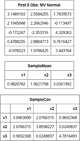
The sample mean is close to the population mean and the sample covariance matrix is close to the population covariance. Just as is true for univariate data, statistics computed on small samples exhibit more variation than statistics on larger samples. Also, the variance of higher-order moments is greater than for lower-order moments.

To visually examine the simulated data, you can write the data to a SAS data set and use the SGSCATTER procedure to create a plot of the univariate and bivariate marginal distributions. Alternatively, you can use the CORR procedure to produce Figure 8.5, as is shown in the following statements. The CORR procedure also produces the sample mean and sample covariance, but these tables are not shown.

/* write SAS/IML matrix to SAS data set for plotting */
create MVN from X[colname=c]; append from X; close MVN; 
quit;

/* create scatter plot matrix of simulated data */ 
ods graphics on;
proc corr data=MVN COV plots(maxpoints=NONE)=matrix(histogram);
    var x:; 
run;

Figure 8.5 Univariate and Bivariate Marginal Distributions for Simulated Multivariate Normal Data

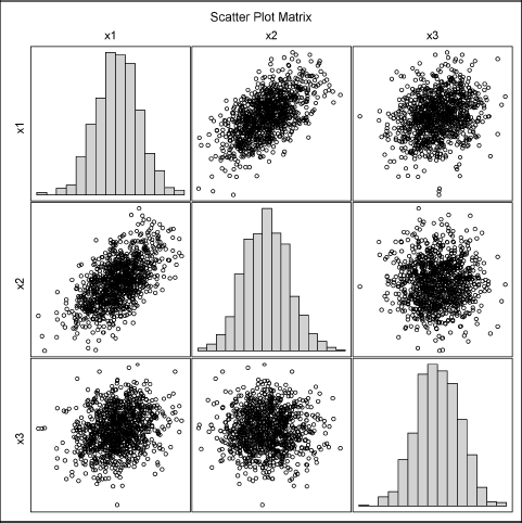
Figure 8.5 shows that the marginal distribution for each variable (displayed as histograms on the diagonal) appears to be normal, as do the pairwise bivariate distributions (displayed as scatter plots). This is characteristic of MVN data: All marginal distributions are normally distributed.

In addition to the graphical checks, there are rigorous goodness-of-fit tests to determine whether data are likely to have come from a multivariate normal distribution. You can search the support.sas.com Web site to find the %MULTNORM macro, which performs tests for multivariate normality. The %MULTNORM macro also computes and plots the squared Mahalanobis distances of the observations to the mean vector. For p-dimensional MVN data, the squared distances are distributed as chi-square with p degrees of freedom. Consequently, a plot of the squared distance versus quantiles of a chi-square distribution will fall along a straight line for data that are multivariate normal.

Exercise 8.2: The numeric variables in the Sashelp.Iris data set are SepalLength, SepalWidth, PetalLength, and PetalWidth. There are three species of flowers in the data. Use PROC CORR to visualize these variables for the “Virginica” species. Do the data appear to be multivariate normal? Repeat the analysis for the “Setosa” species.

8.3.2 Simulating Multivariate Normal Data in SAS/STAT Software

A second way to generate MVN data is to use the SIMNORMAL procedure in SAS/STAT software. As is shown in Section 8.3.1, you must provide the mean and covariance of the distribution in order to simulate the data. For PROC SIMNORMAL, this is accomplished by creating a TYPE=COV data set, as shown in the following example:

/* create a TYPE=COV data set */
data MyCov(type=COV);
input _TYPE_ $ 1-8 _NAME_ $ 9-16 x1 x2 x3;
datalines;
COV      x1     3 2 1
COV      x2     2 4 0
COV      x3     1 0 5
MEAN            1 2 3
run;

The data set specifies the same mean vector and covariance matrix as the example in Section 8.3.1. This data set is used as the input data for the SIMNORMAL procedure. For example, the following call generates 1,000 random observations from the MVN distribution with the specified mean and covariance:

proc simnormal data=MyCov outsim=MVN
      nr = 1000       /* size of sample */
      seed =12345;    /* random number seed */
   var x1-x3; 
run;

The SIMNORMAL procedure does not produce any tables; it only creates the output data set that contains the simulated data. You can run PROC CORR and the %MULTNORM macro to convince yourself that the output of PROC SIMNORMAL is multivariate normal from the specified distribution.

The SIMNORMAL procedure also enables you to perform conditional simulation from an MVN distribution. Given an MVN distribution with p variables, you can specify the values of k < p variables and simulate the remaining p – k, conditioned on the specified values. See Section 8.6 for more information about conditional simulation.

Exercise 8.3: Use PROC CORR and the %MULTNORM macro to analyze the simulated data in the MVN data set.

8.4 Generating Data from Other Multivariate Distributions

SAS/IML software supports several other multivariate distributions:

• The RANDDIRICHLET function generates a random sample from a Dirichlet distribution, which is not used in this book.
• The RANDMVT function generates a random sample from a multivariate Student's t distribution (Kotz and Nadarajah 2004).
• The RANDWISHART function, which is described in Section 10.5, generates a random sample from a Wishart distribution.

Johnson (1987) presents many other (lesser-known) multivariate distributions and describes simulation techniques for generating multivariate data. There are also multivariate distributions mentioned in Gentle (2003).

The multivariate Student's t distribution is useful when you want to simulate data from a multivariate distribution that is similar to the MVN distribution, but has fatter tails. The multivariate t distribution with v degrees of freedom has marginal distributions that are univariate t with v degrees of freedom.

The SAS/IML RANDMVT function simulates data from a multivariate t distribution. The syntax of the RANDMVT function is

X = RandMVT(NumSamples, DF, Mean, S);

where NumSamples is the number of observations in the sample, DF is the degrees of freedom, Mean is a 1 × p vector, and S is a p × p positive definite matrix. Given the matrix S, the population covariance is where v > 2 is the degrees of freedom. For large values of v, the multivariate t distribution is approximately multivariate normal.

The following statements generate a 100 × 3 matrix, where each row is a random observation from a multivariate t distribution with 4 degrees of freedom:

proc iml;
/* specify population mean and covariance */ 
Mean = {1, 2, 3}; 
Cov = {3 2 1,
       2 4 0, 
       1 0 5}; 
call randseed(4321);
X = RandMVT(100, 4, Mean, Cov);   /* 100 draws; 4 degrees of freedom */

Exercise 8.4: Use PROC CORR to compute the sample correlations and to visualize the distribution of the multivariate t data with four degrees of freedom. Can you see evidence that the tails of the t distribution are heavier than for the normal distribution?

8.5 Mixtures of Multivariate Distributions

As was described in Section 7.5 for univariate distributions, you can simulate multivariate data from a mixture of other distributions. This is useful, for example, for simulating clustered data and data for discriminant analysis.

8.5.1 The Multivariate Contaminated Normal Distribution

The multivariate contaminated normal distribution is similar to the univariate version that is presented in Section 7.5.2. Given a mean vector μ and a covariance matrix Σ, you can sample from an MVN(μ, Σ) distribution with probability 1 – p and from an MVN(μ, k²Σ) distribution with probability p, where k > 1 is a constant that represents the size of the contaminated component. This results in a distribution with heavier tails than normality. This is also a convenient way to generate data with outliers.

The following SAS/IML statements call the RANDNORMAL function to generate N₁ observations from MVN(μ, Σ) and N – N₁ observations from MVN(μ, k²Σ), where N₁ is chosen randomly from a binomial distribution with parameter 1 – p:

/* create multivariate contaminated normal distrib */
%let N = 100; 
proc iml;
mu = {0 0 0};       /* vector of means */
Cov = {10 3 -2,
        3 6 1, 
       -2 1 2};
k2 = 100;           /* contamination factor */
p = 0.1;            /* prob of contamination */

/* generate contaminated normal (mixture) distribution */
call randseed(1);
call randgen(N1, “Binomial”, 1-p, &N); /* N1 unallocated ==> scalar */

X = j(&N, ncol(mu));
X[1:N1,] = RandNormal(N1, mu, Cov);           /* uncontaminated */
X[N1+1:&N,] = RandNormal(&N-N1, mu, k2*Cov);   /* contaminated */

Notice that the program only makes two calls to the RANDNORMAL function. This is more efficient than writing a DO loop that iteratively draws a Bernoulli random variable and simulates a single observation from the selected distribution.

You can create a SAS data set and use PROC CORR to visualize the simulated data. Figure 8.7 shows the scatter plot matrix of the three variables.

/* write SAS data set */
create Contam from X[c=(‘x1’:‘x3’)]; append from X; close Contam; 
quit;

proc corr data=Contam cov plots=matrix(histogram);
   var x1-x3; 
run;

Figure 8.6 Analysis of Contaminated Multivariate Normal Data

Figure 8.7 Multivariate Normal Data with 10% Contamination

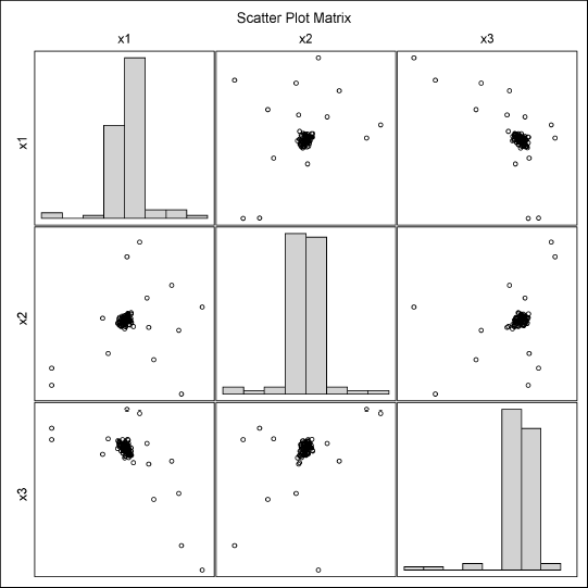
The plots show the high density of observations near the center of each scatter plot. These observations were primarily drawn from the uncontaminated distribution. The remaining observations are from the distribution with the larger variance.

Notice that the covariance estimates that are found by the CORR procedure (see Figure 8.6) are far from the values of the uncontaminated parameters. You can use the MCD subroutine in the SAS/IML language or the ROBUSTREG routine in SAS/STAT software to estimate the covariance parameters in ways that are robust to the presence of outliers.

Exercise 8.5: Use the %MULTNORM macro to test the data in the Contam data set for multivariate normality. Does the chi-square Q-Q plot reveal the presence of two distributions?

8.5.2 Mixtures of Multivariate Normal Distributions

It is easy to extend the contaminated normal example to simulate data from a mixture of k MVN distributions. Suppose that you want to generate N observations from a mixture distribution where each observation has probability π_i of being drawn from MVN(μ_i, Σ_i), i = 1 … k. The following program uses the multinomial distribution (see Section 8.2) to randomly produce N_i, which is the number of observations to be simulated from the i th component distribution:

proc iml;
call randseed(12345);
pi = {0.35 0.5 0.15};   /* mixing probs for k groups */
NumObs = 100;           /* total num obs to sample */
N = RandMultinomial(1, NumObs, pi);
print N;

Figure 8.8 A Draw from the Multinomial Distribution

The following statements continue the program. The mean vectors and covariance matrices are stored as rows of a matrix, and only the lower triangular portion of each covariance matrix is stored. A row is converted to a matrix by calling the SQRVECH function; see Section 10.4.2. For the i th group, you can generate N[i] observations from MVN(μ_i, Σ_i), i = 1 … 3.

varNames={“x1” “x2” “x3”};
mu = {32 16 5,             /* means of Group 1 */
      30 8 4,              /* means of Group 2 */ 
      49 7 5};             /* means of Group 3 */
/* specify lower-triangular within-group covariances */ 
/* c11 c21 c31 c22 c32 c33 */
Cov = {17 7 3 5 1 1,       /* cov of Group 1 */
       90 27 16 9 5 4,     /* cov of Group 2 */
       103 16 11 4 2 2};   /* cov of Group 3 */
/* generate mixture distribution: Sample from
   MVN(mu[i,], Cov[i,]) with probability pi[i] */
p = ncol(pi);              /* number of variables */
X = j(NumObs, p);
Group = j(NumObs, 1);
b = 1;                     /* beginning index */
do i = 1 to p; 
   e = b + N[i] - 1;       /* ending index */
   c = sqrvech(Cov[i,]);   /* cov of group (dense) */ 
   X[b:e, ] = RandNormal(N[i], mu[i,], c);    /* i_th MVN sample */
   Group[b:e] = i; 
   b = e + 1;      /* next group starts at this index */ 
end;

/* save to data set */ 
Y = Group || X;
create F from Y[c=(“Group” || varNames)]; append from Y; close F; 
quit;

proc sgscatter data=F;
   compare y=x2 x=(x1 x3) / group=Group markerattrs=(Size=12); 
run;

Figure 8.9 Grouped Data from MVN Distributions

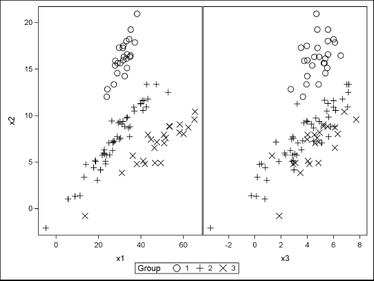
The SGSCATTER procedure is used to visualize the simulated data. The graphs show that there is separation between the groups in the x₁ and x₂ variables because the first two components of the mean vectors are far apart relative to the covariances. However, there is little separation in the x₂ and x₃ variables.

Exercise 8.6: Encapsulate the SAS/IML statements into a function that generates N random observations from a mixture of MVN distributions.

8.6 Conditional Multivariate Normal Distributions

A conditional distribution is the distribution that results when several variables are fixed at some specific value. If f(x₁, x₂,…, x_p) is a probability distribution for p variables, then the conditional probability distribution at x_p = a is f(x₁, x₂,…, a). That is, you substitute the known value. Geometrically, the conditional distribution is obtained by slicing the full distribution with the hyperplane x_p = a. You can also form a conditional distribution by specifying the value of more than one variable. For example, you can specify a k-dimensional conditional distribution by g(x₁, x₂,…, x_k) = f(x₁, x₂,…, k, a_k+1,…, a_p).

For some multivariate distributions, it is difficult to sample from a conditional distribution. Although it is easy to obtain the density function (just substitute the specified values), the resulting density might not be a familiar “named” distribution such as the normal, gamma, or beta distribution.

However, conditional distributions for the MVN distribution are easy to generate because every conditional distribution is also MVN and you can compute the conditional mean and covariance matrix directly (Johnson 1987, p. 50). In particular, let X ~ MVN(μ, Σ), where

The vector X₁ is k × 1, X₂ is (p – k) × 1, Σ₁₁ is k × k, Σ₂₂ is (p – k) × (p – k), and is k × (p – k).

The distribution of X₁, given that X₂ = v, is where

and

You can use the SIMNORMAL procedure to carry out conditional simulation. See the documentation in the SAS/STAT User's Guide for details and an example. In addition, the following SAS/IML program defines a module to compute the conditional mean and covariance matrix, given values for the last k variables, 0 < k < p.

proc iml;
/* Given a p-dimensional MVN distribution and p-k fixed values for 
   the variables x_{k+1},…, x_p, return the conditional mean and 
   covariance for first k variables, conditioned on the last p-k 
   variables. The conditional mean is returned as a column vector. */ 
start CondMVNMeanCov(m, S, _mu, Sigma, _v); 
   mu = colvec(_mu); v = colvec(_v); 
   p = nrow(mu);     k = p - nrow(v);
   mu1 = mu[1:k];
   mu2 = mu[k+1:p];
   Sigma11 = Sigma[1:k, 1:k];
   Sigma12 = Sigma[1:k, k+1:p]; *Sigma21 = T(Sigma12); 
   Sigma22 = Sigma[k+1:p, k+1:p]; 
   m = mu1 + Sigma12*solve(Sigma22, (v - mu2)); 
   S = Sigma11 - Sigma12*solve(Sigma22, Sigma12`); 
finish;

The module returns the conditional mean in the first argument and the conditional covariance in the second argument. To demonstrate how the module works, the following example sets x₃ = 2. The conditional mean and covariance are shown in Figure 8.10.

mu = {1 2 3};   /* 3D MVN example */
Sigma = {3 2 1, 
         2 4 0, 
         1 0 9};
v3 = 2;         /* value of x3 */
run CondMVNMeanCov(m, c, mu, Sigma, v3); 
print m c;

Figure 8.10 Conditional Mean and Covariance

Notice that the second component of the conditional mean is 2, which is the same as for the unconditional mean because X₂ and X₃ are uncorrelated. Similarly, the second column of the conditional covariance is the same ({2 4}) as for the unconditional covariance. However, the first component of the conditional mean is different from the unconditional value because X₁ and X₃ are correlated.

You can use the conditional means and covariances to simulate observations from the conditional distribution: Simply call the RANDNORMAL function with the conditional parameter values, as shown in the following example:

/* Given a p-dimensional MVN distribution and p-k fixed values 
   for the variables x_{k+1}, …, x_p, simulate first k 
   variables conditioned on the last p-k variables. */ 
start CondMVN(N, mu, Sigma, v);
   run CondMVNMeanCov(m, S, mu, Sigma, v);
   return( RandNormal(N, m`, S) );   /* m` is row vector */
finish;

call randseed(1234); 
N = 1000;
z = CondMVN(N, mu, Sigma, v3);   /* simulate 2D conditional distrib */

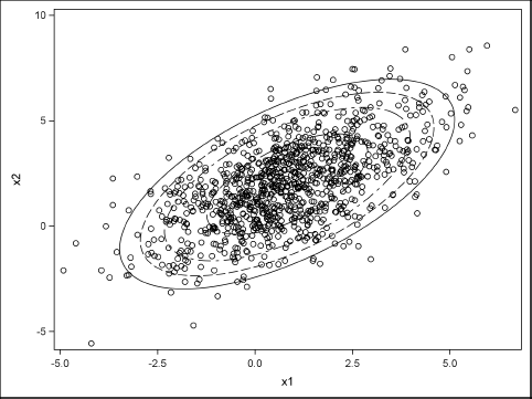
You can write the data to a SAS data set and plot it by using the SGPLOT procedure. The following statements also overlay bivariate normal probability ellipses on the simulated data:

varNames = “x1”:“x2”;
create mvn2 from z[c=varNames]; append from z; close mvn2; 
quit;

proc sgplot data=mvn2 noautolegend; 
   scatter x=x1 y=x2; 
   ellipse x=x1 y=x2 / alpha=0.05; 
   ellipse x=x1 y=x2 / alpha=0.1; 
   ellipse x=x1 y=x2 / alpha=0.2; 
   ellipse x=x1 y=x2 / alpha=0.5; 
run;

Figure 8.11 Simulated Data from Conditional MVN Distribution

Exercise 8.7: Call the CondMVNMeanCov function with the input v = {2, 3}. What is the mean and variance of the resulting conditional distribution? Call the CondMVN function with the same input. Simulate 1,000 observations from the conditional distribution and create a histogram of the simulated data.

8.7 Methods for Generating Data from Multivariate Distributions

Generating data from multivariate distributions with correlated components and specified marginal distributions is hard. There have been many papers written about how to simulate from multivariate distributions that have certain properties. Relatively few general techniques exist for simulating data that have both a target correlation structure and specified marginal distributions. One reason is that if you specify the marginal distributions arbitrarily, then some correlation structures are unobtainable.

The simulation literature contains three general techniques that are used frequently. They are the conditional distribution technique, the transformation technique, and the copula technique, which combines features of the first two techniques. The conditional distribution and transformation techniques are described in Johnson (1987), which is used as the basis for the notation and ideas in this section. The copula technique is described in Section 9.5.

8.7.1 The Conditional Distribution Technique

The goal of a multivariate simulation is to generate observations from a p-dimensional distribution. Each observation is the realization of some random vector X = (X₁, X₂, … , X_p). The conditional distribution technique converts the problem into a sequence of p one-dimensional problems. You generate an observation x = (x₁, x₂, … , x_p) by doing the following:

1. Generate x₁ from the marginal distribution of X₁.
2. For k = 2, … , p, generate X_k from the conditional distribution of X_k, given X₁ = x₁, X₂ = x₂, … , X_k–1 = x_k–1.

One problem with this method is that it might be difficult to compute a random variate from the conditional distributions. You might not be able to express the conditional distributions in an exact form because they can be complicated functions of the previous variates. Another problem is that conditional techniques tend to be much slower than direct techniques. However, an advantage is that the conditional technique is broadly applicable, even in very high dimensions. The conditional distribution technique is the basis for Gibbs sampling, which is available for Bayesian modeling in the MCMC procedure in SAS/STAT software.

As an example, you can use the formulas shown in Section 8.6 to generate data from a conditional MVN distribution by using the CondMVNMeanCov module multiple times. For example, for three-dimensional data, you can generate a single observation by doing the following:

1. Generate x₃ from a univariate normal distribution with mean μ₃ and variance Σ₃₃. Pass this x₃ value into the CondMVNMeanCov module to get a two-dimensional conditional mean, v, and covariance matrix, A.
2. Generate x₂ from a univariate normal distribution with mean v₂ and variance A₂₂. Pass this x₂ value into the CondMVNMeanCov module to get a one-dimensional conditional mean and covariance matrix.
3. Generate x₁ from a univariate normal distribution with the mean and variance found in the previous step.

For the MVN distribution, this technique is not as efficient as the transformation technique that is shown in Section 8.7.2. However, it demonstrates that the conditional distribution technique enables you to sample from a multivariate distribution by sampling one variable at a time.

Exercise 8.8: Write a SAS/IML function that uses the conditional technique to simulate from the three-dimensional MVN distribution that is specified in Section 8.6. Compare the time it takes to simulate 10,000 observations by using the conditional distribution technique with the time it takes to generate the same number of observations by using the RANDNORMAL function.

8.7.2 The Transformation Technique

Often the conditional distributions of a multivariate distribution are difficult to compute. A second technique for generating multivariate samples is to generate p values from independent univariate distributions and transform those values to have the properties of the desired multivariate distribution. This transformation technique is widely used. For example, many of the algorithms in Devroye (1986) use this technique.

Section 7.3 provides univariate examples that use the transformation technique. The beauty of the technique is that many distributions can be generated by using independent uniform or normal distribution as the basis for the (pre-transformed) data. For example, Johnson (1987) mentions that the multivariate Cauchy distribution can also be generated from standard normal distributions and a Gamma(1/2) distribution. Specifically, if Z_i is a standard normal variable, i = 1,…, p, and Y is a Gamma(1/2) variable, then you can generate the multivariate Cauchy distribution from as shown in the following SAS/IML module. Notice that the module is vectorized: All N observations for all p normal variables are generated in a single call, as are all N Gamma(1/2) variates.

proc iml;
/* Sample from a multivariate Cauchy distribution */ 
start RandMVCauchy(N, p);
    z = j(N, p, 0); y = j(N, 1);        /* allocate matrix and vector */
    call randgen(z, “Normal”);
    call randgen(y, “Gamma”, 0.5);   /* alpha=0.5, unit scale */
    return( z / sqrt(2*y) ); 
finish;

/* call the function to generate multivariate Cauchy variates */ 
N=1000; p = 3; 
x = RandMVCauchy(N, p);

The transformation technique generates the data directly; there is no iteration as in the conditional simulation technique.

8.8 The Cholesky Transformation

The RANDNORMAL function that is discussed in Section 8.3.1 uses a technique known as the Cholesky transformation to simulate MVN data from a population with a given covariance structure. This section describes the Cholesky transformation and its geometric properties. This transformation is often used as part of an algorithm to generate correlated multivariate data from a wide range of distributions.

A covariance matrix, Σ, contains the covariances between random variables: Σ_ij = Cov(X_i, X_j). You can transform a set of uncorrelated variables into variables with the given covariances. The transformation that accomplishes this task is called the Cholesky transformation; it is represented by a matrix that is a “square root” of the covariance matrix.

Any covariance matrix, Σ, can be factored uniquely into a product Σ = U^T U, where U is an upper triangular matrix with positive diagonal entries and the superscript denotes matrix transpose. The matrix U is the Cholesky (or “square root”) matrix. Some researchers such as Golub and Van Loan (Golub and Van Loan 1989, p. 143) prefer to work with lower triangular matrices. If you define L = U^T, then Σ = LL^T. Golub and Van Loan provide a proof of the Cholesky decomposition, as well as various ways to compute it. In SAS/IML software, the Cholesky decomposition is computed by using the ROOT function.

The Cholesky matrix transforms uncorrelated variables into variables whose variances and covariances are given by Σ. In particular, if you generate p standard normal variates, the Cholesky transformation maps the variables into variables for the MVN distribution with covariance matrix Σ and centered at the origin (denoted MVN(0, Σ)).

For a simple example, suppose that you want to generate MVN data that are uncorrelated, but have non-unit variance. The covariance matrix for this situation is the diagonal matrix of variances: Σ = diag(σ₁², … , σ_p²). The square root of Σ is the diagonal matrix D that consists of the standard deviations: Σ = D^TD where D = diag(σ₁, … , σ_p).

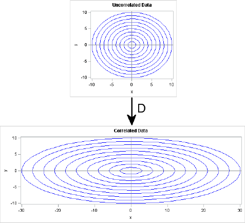
Geometrically, the D matrix scales each coordinate direction independently of the other directions. This is shown in Figure 8.12. The horizontal axis is scaled by a factor of 3, whereas the vertical axis is unchanged (scale factor of 1). The transformation is D = diag(3,1), which corresponds to a covariance matrix of diag(9,1). If you think of the circles in the top image as being probability contours for the multivariate distribution MVN(0, I), then the bottom shows the corresponding probability ellipses for the distribution MVN(0, D).

Figure 8.12 The Geometry of a Diagonal Transformation

In the general case, a covariance matrix contains off-diagonal elements. The geometry of the Cholesky transformation is similar to the pure-scaling case shown previously, but also shears and rotates the top image.

Computing a Cholesky matrix for a general covariance matrix is not as simple as computing a Cholesky matrix for a diagonal covariance matrix. In SAS/IML software, the ROOT function returns a matrix U such that the product U^T U equals the covariance matrix, and U is an upper triangular matrix with positive diagonal entries. The following statements compute a Cholesky matrix in PROC IML:

proc iml; 
Sigma = {9 1,
         1 1}; 
U = root(Sigma);
print U[format=BEST5.];    /* U`*U = Sigma */

Figure 8.13 A Cholesky Matrix

You can use the Cholesky matrix to create correlations among random variables. For example, suppose that X and Y are independent standard normal variables. The matrix U (or its transpose, L = U^T) can be used to create new variables Z and W such that the covariance of Z and W equals Σ. The following SAS/IML statements generate X and Y as rows of the matrix xy. That is, each column is a point (x, y). (Usually the columns of a matrix are used to store variables, but transposing xy makes the linear algebra simpler.) The statements then map each (x, y) pair to a new point, (z, w), and compute the sample covariance of the Z and W variables. As promised, the sample covariance is close to Σ, which is the covariance of the underlying population.

/* generate x, y ~ N(0, 1), corr(x, y)=0 */ 
call randseed(12345); 
xy = j(2, 1000);
call randgen(xy, “Normal”); /* each col is indep N(0,1) */

L = U`;
zw = L * xy;    /* Cholesky transformation induces correlation */
cov = cov(zw`); /* check covariance of transformed variables */
print cov[format=BEST5.];

Figure 8.14 Sample Covariance Matrix

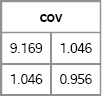
Figure 8.15 shows the geometry of the transformation in terms of the data and in terms of probability ellipses. The top image is a scatter plot of the X and Y variables. Notice that they are uncorrelated and that the probability ellipses are circles. The bottom image is a scatter plot of the Z and W variables. Notice that they are correlated and the probability contours are ellipses that are tilted with respect to the coordinate axes. The bottom image is the transformation under L of the points and circles in the top image.

Figure 8.15 The Geometry of a Cholesky Transformation

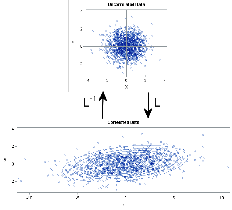
It is also possible to “uncorrelate” correlated variables, and the transformation that uncorrelates variables is the inverse of the Cholesky transformation. Specifically, if you generate data from MVN(0,Σ), you can uncorrelate the data by applying L^–1. In SAS/IML software, you might be tempted to use the INV function to compute an explicit matrix inverse, but this is not efficient (Wicklin 2010, p. 372). Because L is a lower triangular matrix, it is more efficient to use the TRISOLV function, as shown in the following statements:

/* Start with MVN(0, Sigma) data. Apply inverse of L. */ 
zw = T( RandNormal(1000, {0, 0}, Sigma) );
xy = trisolv(4, L, zw);   /* more efficient than solve(L, zw) */

/* Did we succeed in uncorrelating the data? Compute covariance. */
tcov = cov(xy`);
print tcov[format=5.3];

Figure 8.16 Covariance of Transformed Data

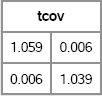
Notice that Figure 8.16 shows that the covariance matrix of the transformed data is close to the identity matrix. The inverse Cholesky transformation has “uncorrelated” the data.

The TRISOLV function, which uses back-substitution to solve the linear system, is extremely fast. Anytime you are trying to solve a linear system that involves a covariance matrix, you should compute the Cholesky factor and use back-substitution to solve the system.

8.9 The Spectral Decomposition

The Cholesky factor is just one way to obtain a “square root” matrix of a correlation matrix. Another option is the spectral decomposition, which is also known as the eigenvalue decomposition. Given a correlation matrix, R, you can factor R as R = UDU' where U is the matrix of eigenvectors and D is a diagonal matrix that contains the eigenvalues. Then the matrix H = D^1/2 U' (called the factor pattern matrix) is a square root matrix of R because H' H = R. Sometimes it is more convenient to work with transposes such as F = H' = UD^1/2.

A factor pattern matrix can be computed by PROC FACTOR or in the SAS/IML language as part of an eigenvalue decomposition of the correlation matrix. For example, the following example is modified from Fan et al. (2002, p. 72):

data A(type=corr); 
_type_=‘CORR’; 
input x1-x3; 
cards;
1.0  .   . 
0.7 1.0  .
0.2 0.4 1.0
;
run;

/* obtain factor pattern matrix from PROC FACTOR */ 
proc factor data=A N=3 eigenvectors;
   ods select FactorPattern; 
run;

/* Perform the same computation in SAS/IML language */ 
proc iml; 
R = {1.0 0.7 0.2, 
     0.7 1.0 0.4, 
     0.2 0.4 1.0};

/* factor pattern matrix via the eigenvalue decomp.
 R = U*diag(D)*U` = H`*H = F*F` */
call eigen(D, U, R);
F = sqrt(D`) # U;   /* F is returned by PROC FACTOR */
Verify = F*F`;
print F[format=8.5] Verify;

Figure 8.17 Factor Pattern Matrix

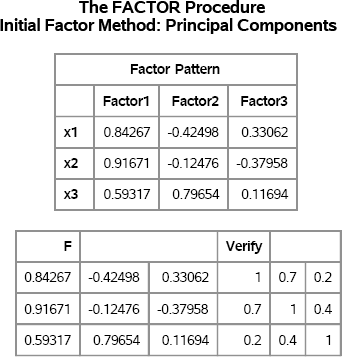
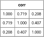
The factor pattern matrix H is a square-root matrix for R. Consequently, H can be used to transform uncorrelated standard normal variates into correlated multivariate normal variates. For example, the following SAS/IML statements simulate from an MVN distribution where the variables are correlated according to the R matrix. Figure 8.18 shows that the columns of x are correlated and the sample correlation is close to R. The spectral decomposition is used in Section 10.8 and Section 16.11.

z = j(1000, 3);
call randgen(z, “Normal”);    /* uncorrelated normal obs: z~MVN(0,I) */

/* Compute x`=F*z` or its transpose x=z*F` */
x = z*F`;                     /* x~MVN(0,R) where R=FF`= corr matrix */
corr = corr(x);               /* sample correlation is close to R */
print corr[format=5.3];

Figure 8.18 Sample Correlation Matrix of Simulated Data

8.10 References

Devroye, L. (1986), Non-uniform Random Variate Generation, New York: Springer-Verlag.
URL http://luc.devroye.org/rnbookindex.html

Fan, X., Felsovályi, A., Sivo, S. A., and Keenan, S. C. (2002), SAS for Monte Carlo Studies: A Guide for Quantitative Researchers, Cary, NC: SAS Institute Inc.

Gentle, J. E. (2003), Random Number Generation and Monte Carlo Methods, 2nd Edition, Berlin: Springer-Verlag.

Golub, G. H. and Van Loan, C. F. (1989), Matrix Computations, 2nd Edition, Baltimore: Johns Hopkins University Press.

Johnson, M. E. (1987), Multivariate Statistical Simulation, New York: John Wiley & Sons.

Kotz, S. and Nadarajah, S. (2004), Multivariate t Distributions and Their Applications, Cambridge: Cambridge University Press.

Wicklin, R. (2010), Statistical Programming with SAS/IML Software, Cary, NC: SAS Institute Inc.