Chapter 10

Building Correlation and Covariance Matrices

Contents

10.1 Overview of Building Correlation and Covariance Matrices

Most of this book is concerned with simulating data. This chapter is different. It describes how to construct correlation and covariance matrices that you can use in the algorithms that are included in other chapters. This chapter addresses three main issues:

• How to construct covariance matrices that have a particular structure.
• How to simulate random matrices that have a particular set of eigenvalues.
• How to find the correlation matrix that is closest to an arbitrary matrix.

Covariance matrices with known structure are important in many applications and are useful for simulating correlated data. Chapter 8, “Simulating Data from Basic Multivariate Distributions,” includes many examples of simulating correlated data. For each example, you must specify a covariance matrix. Furthermore, correlated data are important in mixed models, time-series models, and spatial models.

Simulating random matrices can be useful for testing algorithms. The second part of this chapter introduces the Wishart distribution, which is the distribution of the sample covariance matrix of the multivariate normal distribution. Section 10.6 shows how to simulate correlation matrices that have specified eigenvalues.

The third part of this chapter discusses what to do when your estimate for a correlation matrix is poor. It might happen that an estimate does not satisfy the mathematical properties that are required for a correlation matrix. Section 10.8 describes one way to adjust your estimate.

All of the correlation matrices in this chapter are Pearson correlations. You can use the Iman-Conover algorithm in Section 9.4 to generate data with a given Spearman rank correlation.

This chapter requires more linear algebra than the rest of the book. The topics are not used heavily in subsequent chapters, so you can skip this material if matrices are not your passion. However, readers who are interested in simulating mixed models should read the chapter through Section 10.4.4.

10.2 Converting between Correlation and Covariance Matrices

Both covariance matrices and correlation matrices are used frequently in multivariate statistics. If S is a covariance matrix, then the corresponding correlation matrix is R = D^–1SD^–1, where D is the diagonal matrix that contains the square root of the diagonal element of S. The diagonal elements of S are the variances of the variables, so D contains the standard deviations of the variables. Although you can use this formula to convert a covariance matrix to a correlation matrix, the following SAS/IML function is an equivalent formulation that is computationally more efficient:

proc iml;
/* convert a covariance matrix, S, to a correlation matrix */ 
start Cov2Corr(S);
   D = sqrt(vecdiag(S));
   return( S / D` / D );       /* divide columns, then divide rows */
finish;

Rather than perform matrix inversion and matrix multiplication, the function divides each column of S by the corresponding element of D, and then divides each row in the same way.

In a similar way, you can convert a correlation matrix into a covariance matrix provided that you know the standard deviations of each variable: S = DRD. The following function is computationally equivalent to the matrix multiplication, but uses scalar multiplication of columns and rows, which is more efficient:

/* R = correlation matrix
   sd = (vector of) standard deviations for each variable 
   Return covariance matrix with sd##2 on the diagonal */ 
start Corr2Cov(R, sd);
   std = colvec(sd);       /* convert to a column vector */
   return( std` # R # std ); 
finish;

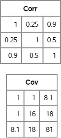
The following statements test these functions. First, define a covariance matrix and convert it to a correlation matrix. Then use the standard deviation of each variable to convert it back to a covariance matrix. Figure 10.1 shows that the process recovers the original covariance matrix.

S = {1.0 1.0 8.1,                /* covariance matrix    */
     1.0 16.0 18.0, 
     8.1 18.0 81.0 }; 
Corr = Cov2Corr(S);              /* convert to correlation matrix */

sd = sqrt(vecdiag(S));           /* sd = {1 4 9}     */
Cov = Corr2Cov(Corr, sd);        /* convert to covariance matrix */
print Corr, Cov;

Figure 10.1 Correlation and Covariance Matrices

In this chapter, some algorithms use a covariance matrix whereas others use a correlation matrix. If necessary, convert the matrix that you have into the form that is required by the algorithm.

10.3 Testing Whether a Matrix Is a Covariance Matrix

When simulating multivariate data, you typically need to provide a covariance (or correlation) matrix to an algorithm that generates the random samples. This is sometimes difficult because not every matrix is a valid covariance matrix. The matrix must be symmetric and positive definite (PD). A positive definite matrix is a matrix that has all positive eigenvalues. A positive semidefinite (PSD) matrix is a matrix that has nonnegative eigenvalues.

Being PSD is equivalent to being a covariance matrix. Every covariance matrix is PSD, and every symmetric PSD matrix is a covariance matrix for some distribution. For brevity, this chapter typically refers to positive definite matrices, although most results and algorithms are also valid for positive semidefinite matrices.

Suppose that you want to test whether a given matrix is a valid covariance matrix. You have to check two properties: that the matrix is symmetric, and that the matrix is positive semidefinite.

10.3.1 Checking Whether a Matrix Is Symmetric

The first step is to check whether the matrix is symmetric. For a small matrix, you can verify symmetry “by eye.” However, for a 100 × 100 matrix, it is better to have the computer check symmetry for you.

Mathematically, a matrix A is symmetric if B = A, where B = (A + A′)/2. However, for finite-precision computations it only makes sense to ask whether max_ij | B_ij – A_ij | is small. The following SAS/IML program checks that the matrix is symmetric to within the scale of the data:

proc iml; 
A = { 2 -1 0, 
     -1 2 -1, 
      0 -1 2 };

/* finite-precision test of whether a matrix is symmetric */ 
start SymCheck(A); 
   B = (A + A`)/2; 
   scale = max(abs(A));
   delta = scale * constant(“SQRTMACEPS”); 
   return( all( abs(B-A)< delta ) ); 
finish;

/* test a matrix for symmetry */ 
IsSym = SymCheck(A); 
print IsSym;

Figure 10.2 Check for Symmetry

Figure 10.2 shows that the SYMCHECK function returns the value 1, which means that the matrix A is symmetric to within numerical precision. The SYMCHECK function uses the CONSTANT function in Base SAS to compute the square root of machine precision (also known as machine epsilon), which is a quantity that is used in numerical analysis to understand the relative error of finite-precision computations.

10.3.2 Checking Whether a Matrix Is Positive Semidefinite

The second step is to check whether a matrix is positive semidefinite. You can use the following SAS/IML functions to test whether a symmetric matrix, A, is PSD:

1. Use the ROOT function to compute a Cholesky decomposition. If the decomposition succeeds, the matrix is PSD.
2. Use the EIGVAL function to compute the eigenvalues of A. If no eigenvalue is negative, A is PSD. If all eigenvalues are positive, A is positive definite.

The ROOT function is faster than the EIGVAL function, so use the ROOT function when you just need a yes-or-no answer, as follows:

G = root(A);

If the matrix is not PSD, the ROOT function will stop with an error: ERROR: Matrix should be positive definite. If the ROOT function does not stop with an error, then the matrix is a valid covariance matrix.

In SAS/IML 12.1 and later, the ROOT function supports an optional second parameter that you can use to suppress the error message. With this syntax, the ROOT function never stops with an ERROR. If A is PSD, then the return value is the Cholesky root of A. Otherwise, the return value is a matrix of missing values. An example follows:

G = root(A, “NoError”);     /* SAS/IML 12.1 and later */
if G=. then print “The matrix is not positive semidefinite”;

Although the EIGVAL function is not as fast as the ROOT function, the EIGVAL function has the advantage that you can inspect the eigenvalues. In particular, the magnitude of the smallest eigenvalue gives information about how close the matrix is to being PSD. A small negative eigenvalue means that the matrix is close to being semidefinite.

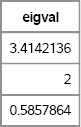
The following statements compute and print the eigenvalues for the example matrix in this section. If any eigenvalue is negative, the matrix is not PSD.

eigval = eigval(A); 
print eigval;
if any(eigval<0) then print “The matrix is not positive semidefinite”;

Figure 10.3 Eigenvalues of a Positive Definite Matrix

10.4 Techniques to Build a Covariance Matrix

Positive definite matrices are special. You cannot write down an arbitrary symmetric matrix and expect it to be PD. This section describes the following techniques for generating a PD covariance or correlation matrix:

• Estimate a covariance matrix from real or simulated data.
• Generate a symmetric matrix that is diagonally dominant.
• Generate a matrix that has a special structure that is known to be PD.

10.4.1 Estimate a Covariance Matrix from Data

If you are trying to simulate data that are similar to a set of real data, it makes sense to use the sample covariance or correlation matrix in the simulation. For example, if you have data that are approximately multivariate normal (MVN), then you can use the estimated covariance matrix in place of the (unknown) population covariance to simulate data.

Two kinds of correlation matrices that arise in practice are the correlation between variables and the correlation between observations.

You can use the CORR procedure to estimate an unstructured empirical correlation of variables. (More sophisticated modelers might use structural equation modeling, which is implemented in the CALIS procedure in SAS/STAT software.) The CORR procedure in Base SAS and the COV function in SAS/IML software can be used to compute covariance matrices for continuous variables. For example, the following statements show two equivalent ways to compute the covariance between numerical variables in the Sashelp.Class data set:

/* Method 1: Base SAS approach */
proc corr data=Sashelp.Class COV NOMISS outp=Pearson; 
     var Age Height Weight; 
     ods select Cov; 
run;

/* Method 2: equivalent SAS/IML computation */ 
proc iml;
use Sashelp.Class;
read all var {“Age” “Height” “Weight”} into X; 
close Sashelp.Class;

Cov = cov(X);

The computations in PROC CORR and PROC IML are equivalent. A covariance matrix that is computed from a data matrix, X, is symmetric positive semidefinite if the following conditions are true:

• No column of X is a linear combination of other columns.
• The number of rows of X exceeds the number of columns.
• If an observation contains a missing value in any variable, then the observation is not used to form the covariance matrix. The NOMISS option in the PROC CORR statement ensures that this condition is satisfied.

In the preceding program, the COV option in the PROC CORR statement is used to generate the covariance matrix. Furthermore, the OUTP= option writes the covariance matrix (and the correlation matrix) to a SAS data set.

In longitudinal studies, observations for the same subject are often correlated. These correlation matrices can be quite large, although they are often assumed to have block form. SAS software supports estimating covariance matrices that have particular structures that arise in repeated measures analyses. The MIXED (or GLIMMIX) procedure can be used for this kind of estimation. See the examples in Section 12.3.

10.4.2 Generating a Symmetric Matrix

Covariance and correlation matrices are symmetric. The first step in generating a random covariance matrix is to know how to generate a symmetric matrix. One way is to generate an arbitrary matrix A and define M = c(A^T + A) for any value of c. However, this method usually changes the distributional properties of the elements. A more efficient approach is to generate the lower triangular portion of a matrix, and then use the SQRVECH function in SAS/IML software to create a full symmetric matrix. (SAS/IML also supports the VECH function, which extracts the lower triangular portion of a square matrix.)

The following SAS/IML program creates a random symmetric matrix where each element is uniformly distributed:

proc iml;
N = 4;                       /* want 4x4 symmetric matrix      */
call randseed(1);
v = j(N*(N+1)/2, 1);         /* allocate lower triangular      */
call randgen(v, “Uniform”);  /* fill with random               */
x = sqrvech(v);              /* create symmetric matrix from v */
print x[format=5.3];

Figure 10.4 A Random Symmetric Matrix

The elements of the matrix x are distributed uniformly; change the argument to the RANDGEN function to simulate elements from other distributions.

10.4.3 Generating a Diagonally Dominant Covariance Matrix

In a simulation study, you might need to generate a random unstructured covariance matrix. For large matrices, if you generate a matrix with unit diagonal for which each off-diagonal element is uniformly and independently generated in [–1, 1], chances are that the matrix is not positive definite. Although every 2 × 2 matrix of this form is a correlation matrix, for 3 × 3 matrices the probability of being PD is 61.7% and for 4 × 4 matrices the probability of being PD drops to 18.3% (Rousseeuw and Molenberghs 1994).

There is a useful fact for creating a PD matrix: A symmetric matrix with positive diagonal entries is PD if it is row diagonally dominant. A matrix A is row diagonally dominant if | A_ii | > Σ_j≠i | A_ij | for each row i . In other words, the magnitude of the diagonal element is greater than the sum of the magnitudes of the off-diagonal elements in the same row.

This means that you can generate an PD matrix by doing the following:

1. Create a random symmetric matrix as shown in Section 10.4.2.
2. For each row, increase the diagonal element until it is larger than the sum of the magnitudes of the other entries.

You can increase the diagonal element of each row independently, but a popular alternative is to find a positive value, λ, such that B = A + λdiag(A) is positive semidefinite. If you define s_i = Σ_j≠i | A_ij | to be the sum of the off-diagonal elements, then B is positive semidefinite provided that λ ≥ max(s_i/d_i) – 1, where d_i is the i th diagonal element. The following SAS/IML module implements this method. The example uses the symmetric 4 × 4 matrix x in Figure 10.4.

/* Add a multiple of diag(A) so that A is diagonally dominant. */ 
start Ridge(A, scale);      /* Input scale >= 1 */
      d = vecdiag(A);
      s = abs(A)[,+] - d;   /* sum(abs of off-diagonal elements) */
      lambda = scale * (max(s/d) - 1); 
      return( A + lambda*diag(d) ); 
finish;

/* assume x is symmetric matrix */
H = Ridge(x, 1.01);         /* scale > 1 ==> H is pos definite */
print H;

Figure 10.5 A Diagonally Dominant Symmetric Matrix

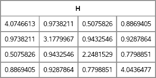
If the scale parameter equals unity, then H is PD. If the parameter is greater than 1, H is positive definite. The matrix H, which is shown in Figure 10.5, is symmetric positive definite, and therefore is a valid covariance matrix. You can confirm that a matrix is PD by using the EIGVAL function to show that the eigenvalues are positive, or by using the ROOT function to compute a Cholesky decomposition.

Exercise 10.1: Write a SAS/IML function that uses the technique in this section to generate N random covariance matrices, where N is a parameter to the function.

Exercise 10.2: Another approach is to define B = A + λ(I). Write a SAS/IML module that takes a matrix A and computes the value of λ so that A + λ(I) is diagonally dominant.

10.4.4 Generating a Covariance Matrix with a Known Structure

There are several well-known covariance structures that are used to model the random effects in mixed models. If you simulate data that are appropriate for a mixed model analysis, it is important to be able to generate covariance matrices with an appropriate structure. Often these structures are used to generate correlated errors from a multivariate normal distribution. See Section 12.3.

This section presents four common covariance structures that are used in mixed modeling and that are supported by the MIXED procedure in SAS: a diagonal structure, compound symmetry, Toeplitz, and first-order autoregressive (AR(1)). Examples of the covariance structures are shown in the following table:

Table 10.1 Covariance Structure Examples

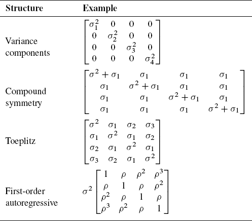
10.4.4.1 A Covariance Matrix with a Diagonal Structure

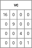
The diagonal covariance matrix is known as the variance components model. It is easy to create such a covariance structure in SAS/IML software, as demonstrated by the following module definition. The matrix shown in Figure 10.6 is a covariance matrix that contains specified variances along the diagonal. As long as the diagonal elements are positive, the resulting matrix is a covariance matrix.

proc iml;
/* variance components: diag({var1, var2,.., varN}), var_i>0 */ 
start VarComp(v);
   return( diag(v) ); 
finish;

vc = VarComp({16,9,4,1}); 
print vc;

Figure 10.6 A Covariance Matrix with Diagonal Structure

10.4.4.2 A Covariance Matrix with Compound Symmetry

The compound symmetry model is the sum of a constant matrix and a diagonal matrix. The compound symmetry structure arises naturally with nested random effects. The following module generates a matrix with compound symmetry. The matrix shown in Figure 10.7 is a compound symmetric matrix. To guarantee that a compound symmetric matrix is PD, choose v > 0 and v₁ > –v/N.

/* compound symmetry, v>0: 
      {v+v1 v1 v1 v1, 
         v1 v+v1 v1 v1, 
         v1 v1 v+v1 v1, 
         v1 v1 v1 v+v1 };
*/
start CompSym(N, v, v1);
   return( j(N, N, v1) + diag( j(N, 1, v) ) ); 
finish;

cs = CompSym(4, 4, 1); 
print cs;

Figure 10.7 A Covariance Matrix with Compound Symmetry Structure

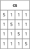
The compound symmetry structure is of the form vI + v₁J, where I is the identity matrix and J is the matrix of all ones. A special case of the compound symmetry structure is the uniform correlation structure, which is a matrix of the form (1 – v₁)I + v₁J. The uniform correlation structure (sometimes called a constant correlation structure) is PD when v₁ > –1/(N – 1).

Exercise 10.3: Write a SAS/IML function that constructs a matrix with uniform correlation structure.

10.4.4.3 A Covariance Matrix with Toeplitz Structure

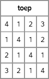
A Toeplitz matrix has a banded structure. The diagonals that are parallel to the main diagonal are constant. The SAS/IML language has a built-in TOEPLITZ function that returns a Toeplitz matrix, as shown in the following example. The matrix shown in Figure 10.8 has a Toeplitz structure. Other than diagonal dominance, there is no simple rule that tells you how to choose the Toeplitz parameters in order to ensure a positive definite matrix.

/* Toeplitz:
      {s##2  s1  s2  s3, 
       s1  s##2  s1  s2, 
       s2  s1  s##2  s1, 
       s3  s2  s1  s##2 }; 
      Let u = {s1 s2 s3};
*/
toep = toeplitz( {4 1 2 3} ); 
print toep;

Figure 10.8 A Covariance Matrix with Toeplitz Structure

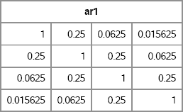
10.4.4.4 A Covariance Matrix with First-Order Autoregressive Structure

A first-order autoregressive (AR(1)) structure is a Toeplitz matrix with additional structure. Whereas an n × n Toeplitz matrix has n parameters, an AR(1) structure has two parameters. The values along each diagonal are related to each other by a multiplicative factor. The following module generates a matrix with AR(1) structure by calling the module in the previous section. The matrix shown in Figure 10.9 has an AR(1) structure. An AR(1) matrix is PD when |ρ| < 1.

/* AR1 is special case of Toeplitz */ 
/* autoregressive(1): 
    s##2 * {1  rho  rho##2  rho##3,
            rho  1  rho  rho##2,
            rho##2  rho  1  rho ,
            rho##3  rho##2  rho  1 };
    Let u = {rho rho##2 rho##3} 
*/
start AR1(N, s, rho);
      u = cuprod(j(1,N-1, rho));       /* cumulative product */
      return( s##2 # toeplitz(1 || u) );
finish;

ar1 = AR1(4, 1, 0.25);
print ar1;

Figure 10.9 A Covariance Matrix with AR(1) Structure

10.5 Generating Matrices from the Wishart Distribution

If you draw N observations from a MVN(0,Σ) distribution and compute the sample covariance matrix, S, then the sample covariance is not exactly equal to the population covariance, Σ. Like all statistics, S has a distribution. The sampling distribution depends on Σ and on the sample size, N.

The Wishart distribution is the sampling distribution of A = (N – 1)S. Equivalently, you can say that A is distributed as a Wishart distribution with N – 1 degrees of freedom, which is written W(Σ, N – 1). Notice that S = (X – )^T (X – )/(N – 1), where X is a sample from MVN(0,Σ) and where is the sample mean. Therefore, A is the scatter matrix (X – )^T (X – ). You can simulate draws from the Wishart distribution by calling the RANDWISHART function in SAS/IML software, as shown in the following program. Two covariance matrices are shown in Figure 10.10.

proc iml;
call randseed(12345);
NumSamples = 1000;                 /* number of Wishart draws       */
N = 50;                            /* MVN sample size               */
Sigma = {9 1, 
               1 1};
/* Simulate matrices. Each row is scatter matrix */ 
A = RandWishart(NumSamples, N-1, Sigma);
B = A / (N-1);                     /* each row is covariance matrix */

S1 = shape(B[1,], 2, 2);           /* first row, reshape into 2 × 2 */
S2 = shape(B[2,], 2, 2);           /* second row, reshape into 2 × 2 */ 
print S1 S2;                       /* two 2 × 2 covariance matrices */

SampleMean = shape(B[:,], 2, 2);   /* mean covariance matrix        */
print SampleMean;

Figure 10.10 Sample Covariance Matrices and Mean Covariance

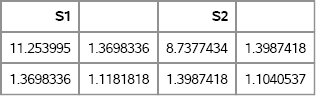
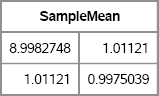
Each row of A is the scatter matrix for a sample of 50 observations drawn from a MVN(0, Σ) distribution. Each row of B is the associated covariance matrix. The SHAPE function is used to convert a row of B into a 2 × 2 matrix. Figure 10.10 shows that the sample variances and covariance are close to the population values, but there is considerable variance in those values due to the small sample, N = 50. If you compute the average of the scatter matrices that are contained in B, you obtain the Monte Carlo estimate of Σ.

Exercise 10.4: Modify the program in this section to write the columns of B to a SAS data set. Use PROC UNIVARIATE to draw histograms of B₁₁, B₁₂, and B₂₂, where B_ij is the (i, j)th element of B. Confirm that the distribution of the estimates are centered around the population parameters. Compare the standard deviations of the diagonal elements of B (the variances) and the off-diagonal element (the covariance).

10.6 Generating Random Correlation Matrices

The “structured” covariance matrices in Section 10.4.4 are useful for generating correlated observations that arise in repeated measures analysis and mixed models. Another useful matrix structure involves eigenvalues. The set of eigenvalues for a matrix is called its spectrum. This section describes how to generate a random correlation matrix with a given spectrum.

The ability to generate a correlation matrix with a specific spectrum is useful in many contexts. For example, in principal component analysis, the k largest eigenvalues of the correlation matrix determine the proportion of the (standardized) variance that is explained by the first k principal components. By specifying the eigenvalues, you can simulate data for which the first k principal components explain a certain percentage of the variance. Another example arises in regression analysis where the ratio of the largest eigenvalue to the other eigenvalues is important in collinearity diagnostics (Belsley, Kuh, and Welsch 1980).

The eigenvalues of an n × n correlation matrix are real, nonnegative, and sum to n because the trace of a matrix is the sum of its eigenvalues. Given those constraints, Davies and Higham (2000) showed how to create a random correlation matrix with a specified spectrum. The algorithm consists of the following steps:

1. Generate a random matrix with the specified eigenvalues. This step requires generating a random orthogonal matrix (Stewart 1980).
2. Apply Givens rotations to convert the random matrix to a correlation matrix without changing the eigenvalues (Bendel and Mickey 1978).

This book's Web site contains a set of SAS/IML functions for generating random correlation matrices. Some of the SAS/IML programs are based on MATLAB functions written by Higham (1991) or GAUSS functions written by Rapuch and Roncalli (2001). You can download and store the functions in a SAS/IML library and use the LOAD statement to read the modules into the active PROC IML session, as follows:

/* Define and store the functions for random correlation matrices */ 
%include “C:<path>RandCorr.sas”;

proc iml;
load module=_all_;      /* load the modules */

The main function is the RANDCORR function, which returns a random correlation matrix with a given set of eigenvalues. The syntax is R = RandCorr(lambda), where lambda is a vector with d elements that specifies the eigenvalues. If the elements of lambda do not sum to d, the vector is scaled appropriately.

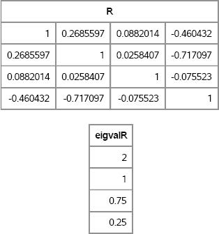
The following statements call the RANDCORR function to create a random correlation matrix with a given set of eigenvalues. The EIGVAL function is called to verify the eigenvalues are correct:

/* test it: generate 4 × 4 matrix with given spectrum */ 
call randseed(4321);
lambda = {2 1 0.75 0.25};   /* notice that sum(lambda) =4 */
R = RandCorr(lambda);       /* R has lambda for eigenvalues */
eigvalR = eigval(R);        /* verify eigenvalues */
print R, eigvalR;

Figure 10.11 Random Correlation Matrix with Specified Eigenvalues

There are many ways to use the random correlation matrix in simulation studies. For example, you can use it to create a TYPE=CORR data set to use as input to a SAS procedure. Or you can use the matrix as an argument to the RANDNORMAL function, as in Section 8.3.1. Or you can use R directly to generate multivariate correlated data, as shown in Section 8.8.

Uncorrelated data have a correlation matrix for which all eigenvalues are close to unity. Highly correlated data have one large eigenvalue and many smaller eigenvalues. There are many possibilities in between.

Exercise 10.5: Simulate 1,000 random 3 × 3 correlation matrices for the vector λ = (1.5, 1, 0.5). Draw histograms for the distribution of the off-diagonal correlations.

10.7 When Is a Correlation Matrix Not a Correlation Matrix?

A problem faced by practicing statisticians, especially in economics and finance, is that sometimes a complete correlation matrix is not known. The reasons vary. Sometimes good estimates exist for correlations between certain pairs variables, but correlations for other pairs are unmeasured or are poor. Any matrix that contains pairwise correlation estimates might not be a true correlation matrix (Rousseeuw and Molenberghs 1994; Walter and Lopez 1999).

10.7.1 An Example from Finance

To give a concrete example, suppose that an analyst predicts that the correlation between certain currencies (such as the dollar, yen, and euro) will have certain values in the coming year:

• The first and second currencies will have correlation ρ₁₂ = 0.3.
• The first and third currencies will have correlation ρ₁₃ = 0.9.
• The second and third currencies will have correlation ρ₂₃ = 0.9.

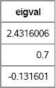
These estimates seem reasonable. Unfortunately, the resulting matrix of correlations is not positive definite and therefore does not represent a valid correlation matrix, as demonstrated by the following program. As shown in Figure 10.12, the matrix has a negative eigenvalue and consequently is not positive definite.

proc iml; 
C = {1.0 0.3 0.9, 
     0.3 1.0 0.9, 
     0.9 0.9 1.0}; 
eigval = eigval(C); 
print eigval;

Figure 10.12 Eigenvalues of an Invalid Correlation Matrix

Mathematically, the problem is that correlations between variables are not independent. They are coupled together by the requirement that a true correlation matrix is positive semidefinite. If R is a correlation matrix, then the correlations must satisfy the condition det(R) ≥ 0. For a 3 × 3 matrix, this implies that the correlation coefficients satisfy

The set of (ρ₁₂, ρ₁₃, ρ₂₃) triplets that satisfy the inequality forms a convex subset of the unit cube (Rousseeuw and Molenberghs 1994). If you substitute ρ₁₂ = 0.3 and ρ₁₃ = ρ₂₃ = 0.9, you will discover that the inequality is not satisfied.

10.7.2 What Causes the Problem and What Can You Do?

Sometimes an estimated sample covariance or correlation matrix is not positive definite. In SAS software, this can occur when the data contain missing values. By default, the CORR procedure computes pairwise correlations, which means that correlations between variables are based on pairs of variables, not on the entire multivariate data. To override the default behavior, use the NOMISS option. The NOMISS option instructs PROC CORR to exclude observations for which any variable is missing, which is a process known as listwise deletion. This option ensures that the resulting covariance matrix is positive semidefinite.

However, if you use listwise deletion and your data contain many missing values, the covariance matrix might be a poor estimate of the population covariance. For example, if 60% of the values for one variable are missing, the covariance computation will be based on a small fraction of the total number of observations in the data.

For a similar reason, indefinite matrices also arise when estimating the polychoric correlations between ordinal variables, regardless of the presence of missing values. SAS distributes a %POLYCHOR macro that constructs a polychoric correlation matrix. (Search the support.sas.com Web site for Sample 25010 to obtain this macro.) The macro documentation states, “The PLCORR option in the FREQ procedure is used iteratively to compute the polychoric correlation for each pair of variables…. The individual correlation coefficients are then assembled” into a matrix. Because the polychoric correlation is computed pairwise, the matrix might be indefinite. (Beginning with SAS 9.3, you can use PROC CORR to compute polychoric correlations; specify the POLYCHORIC option in the PROC CORR statement.)

The following options can be used to convert a matrix that is not positive definite into a matrix that is positive definite:

• One option, which is discussed in Section 10.4.3, is to increase the diagonal values of the covariance estimate by using a so-called ridge factor (Schafer 1997, p. 155). This results in a matrix that is diagonally dominant and therefore PD.
• A second option is to use various algorithms that are collectively known as shrinkage methods (Ledoit and Wolf 2004; Schäfer and Strimmer 2005). The idea is to choose a target matrix, T , which is known to be PD. (The target matrix usually has structure, such as a diagonal or compound symmetric matrix.) The sample covariance matrix, S is then “shrunk” towards the target matrix by using the linear transformation λT + (1 – λ)S. This approach is not presented in this book.
• A third option is to compute the pairwise covariance matrix and, if it is not PD, find the nearest PD matrix to it (Higham 1988, 2002). This approach is popular among some researchers in finance and econometrics. This approach is presented in Section 10.8.

There are disadvantages to each method. Ridge factors and shrinkage are ad-hoc approaches that can result in a covariance matrix that is far from the data-based estimate. The Higham approach does not preserve the covariance structure of a matrix.

The next section presents an algorithm by Nick Higham (Higham 1988, 2002) that finds the closest correlation matrix (in some norm) to a given estimate. The original estimate does not, itself, need to be a valid correlation matrix.

10.8 The Nearest Correlation Matrix

The previous section demonstrated that not every symmetric matrix with unit diagonal is a correlation matrix. If you have an estimated correlation matrix that is not positive semidefinite, then you can try to project it onto the set of true correlation matrices.

Higham's method for finding the nearest correlation matrix consists of a series of alternating projections onto two sets: the set S of symmetric positive semidefinite matrices (which is actually an algebraic variety) and the set U of symmetric matrices with unit diagonals. The intersection of these two sets is the set of correlation matrices, and it is somewhat remarkable that Higham showed (using results of J. Boyle and R. Dykstra) that the alternating projections converge onto the intersection.

To project a matrix X onto the set of positive semidefinite matrices, use the spectral decomposition (see Section 8.9) to decompose the matrix as X = QDQ' where Q is the matrix of eigenvectors and D is a diagonal matrix that contains the eigenvalues. Replace any negative eigenvalues with zeros and then “reassemble” the matrix, as shown in the following SAS/IML function:

proc iml;
/* Project symmetric X onto S={positive semidefinite matrices}.
   Replace any negative eigenvalues of X with zero */ 
start ProjS(X);
   call eigen(D, Q, X);      /* notice that X = Q*D*Q` */
   V = choose(D>0, D, 0);
   W = Q#sqrt(V` );          /* form Q*diag(V)*Q` */
   return( W*W` );           /* W*WV = Q*diag(V)*Q` */
finish;

The projection of a matrix onto the set of matrices with unit diagonal is even easier: merely replace each of the diagonal elements with 1:

/* project square X onto U={matrices with unit diagonal}.
   Return X with the diagonal elements replaced by ones. */ 
start ProjU(X); 
   n = nrow(X);
   Y = X;
   Y[do(1, n*n, n+1)] = 1;      /* set diagonal elements to 1 */
   return ( Y ); 
finish;

The main algorithm consists of calling the PROJS and PROJU functions in a loop. The simplest implementation would just call these functions 100 times and hope for the best. The following implementation keeps track of the process and stops the algorithm when the matrix has converged (within some tolerance) to a correlation matrix:

/* the matrix infinity norm is the max abs value of the row sums */ 
start MatInfNorm(A);
      return( max(abs(A[,+])) ); 
finish;

/* Given a symmetric matrix, A, project A onto the space of PSD 
    matrices. The function uses the algorithm of Higham (2002) to 
    return the matrix X that is closest to A in the Frobenius norm. */ 
start NearestCorr(A);
    maxiter = 100; tol = 1e-8;    /* initialize parameters */
    iter = 1; maxd =1;            /* initial values */
    Yold = A; Xold = A; dS = 0;

    do while( (iter <= maxiter) & (maxd > tol) );
       R = Yold - dS;             /* dS is Dykstra's correction */
       X = ProjS(R);              /* project onto S={PSD} */ 
       dS = X - R;
       Y = ProjU(X);              /* project onto U={Unit diag} */

       /* How much has X changed? (Eqn 4.1) */ 
       dx = MatInfNorm(X-Xold) / MatInfNorm(X); 
       dy = MatInfNorm(Y-Yold) / MatInfNorm(Y); 
       dxy = MatInfNorm(Y - X) / MatInfNorm(Y); 
       maxd = max(dx, dy, dxy); 
       iter = iter + 1;
       Xold = X; Yold = Y;         /* update matrices */
    end;
    return( X );                  /* X is positive semidefinite */
finish;

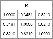
You can test the algorithm on the matrix of pairwise currency correlations. As shown in Figure 10.13, the correlation matrix has off-diagonal entries that are close to the candidate matrix, C. By slightly modifying the candidate matrix, you can obtain a true correlation matrix that can be used to simulate data with the given correlations.

/* finance example */ 
C = {1.0 0.3 0.9, 
     0.3 1.0 0.9, 
     0.9 0.9 1.0}; 
R = NearestCorr(C); 
print R[format=7.4];

Figure 10.13 Nearest Correlation Matrix

The computational cost of Higham's algorithm is dominated by the eigenvalue decomposition. For symmetric matrices, the SAS/IML EIGEN routine is an O(n³) operation, where n is the number of rows in the matrix. For small to medium-sized symmetric matrices (for example, less than 1,000 rows) the EIGEN routine in SAS/IML computes the eigenvalues in a second or two. For larger matrices (for example, 2,000 rows), the eigenvalue decomposition might take 30 seconds or more.

For large matrices (for example, more than 100 rows and columns), you might discover that the numerical computation of the eigenvalues is subject to numerical rounding errors. In other words, if you compute the numerical eigenvalues of a matrix, A, there might be some very small negative eigenvalues, such as –1 × 10^–14. If this interferes with your statistical method and SAS still complains that the matrix is not positive definite, then you can increase the eigenvalues by adding a small multiple of the identity, such as B = ∊I + A, where ∊ is a small positive value chosen so that all eigenvalues of B are positive. Of course, B is not a correlation matrix, because it does not have ones on the diagonal, so you need to convert it to a correlation matrix. It turns out that this combined operation is equivalent to dividing the off-diagonal elements by 1 + ∊, as follows:

/* for large matrices, might need to correct for rounding errors */
eps = 1e-10;
B = ProjU( A/(1+eps) );      /* divide off-diag elements by 1+eps */

Higham's algorithm is very useful. It is guaranteed to converge, although the rate of convergence is linear. A subsequent paper by Borsdorf and Higham (2010) uses a Newton method to achieve quadratic convergence.

Exercise 10.6: Use the method in Section 10.4.2 to generate a random symmetric matrix of size n. Run Higham's algorithm and time how long it takes for n = 50, 100, 150, … 300. Plot the time versus the matrix size.

10.9 References

Belsley, D. A., Kuh, E., and Welsch, R. E. (1980), Regression Diagnostics: Identifying Influential Data and Sources of Collinearity, New York: John Wiley & Sons.

Bendel, R. B. and Mickey, M. R. (1978), “Population Correlation Matrices for Sampling Experiments,” Communications in Statistics—Simulation and Computation, 7, 163-182.

Borsdorf, R. and Higham, N. J. (2010), “A Preconditioned Newton Algorithm for the Nearest Correlation Matrix,” IMA Journal of Numerical Analysis, 30, 94-107.

Davies, P. I. and Higham, N. J. (2000), “Numerically Stable Generation of Correlation Matrices and Their Factors,” BIT, 40, 640-651.

Higham, N. J. (1988), “Computing a Nearest Symmetric Positive Semidefinite Matrix,” Linear Algebra and Its Applications, 103, 103-118.

Higham, N. J. (1991), “Algorithm 694: A Collection of Test Matrices in MATLAB,” ACM Transactions on Mathematical Software, 17, 289-305.
URL http://www.netlib.org/toms/694

Higham, N. J. (2002), “Computing the Nearest Correlation Matrix—a Problem from Finance,” IMA Journal of Numerical Analysis, 22, 329-343.

Ledoit, O. and Wolf, M. (2004), “Honey, I Shrunk the Sample Covariance Matrix,” Journal of Portfolio Management, 30, 110-119.
URL http://ssrn.com/abstract=433840

Rapuch, G. and Roncalli, T. (2001), “GAUSS Procedures for Computing the Nearest Correlation Matrix and Simulating Correlation Matrices,” Groupe de Recherche Opérationelle, Crédit Lyonnais.
URL http://thierry-roncalli.com/download/gauss-corr.pdf

Rousseeuw, P. J. and Molenberghs, G. (1994), “The Shape of Correlation Matrices,” American Statistician, 48, 276-279.
URL http://www.jstor.org/stable/2684832

Schäfer, J. and Strimmer, K. (2005), “A Shrinkage Approach to Large-Scale Covariance Matrix Estimation and Implications for Functional Genomics,” Statistical Applications in Genetics and Molecular Biology, 4.
URL http://uni-leipzig.de/~strimmer/lab/publications/journals/shrinkcov2005.pdf

Schafer, J. L. (1997), Analysis of Incomplete Multivariate Data, New York: Chapman & Hall.

Stewart, G. W. (1980), “The Efficient Generation of Random Orthogonal Matrices with an Application to Condition Estimators,” SIAM Journal on Numerical Analysis, 17, 403-409.
URL http://www.jstor.org/stable/2156882

Walter, C. and Lopez, J. A. (1999), “The Shape of Things in a Currency Trio,” Federal Reserve Bank of San Francisco Working Paper Series, Paper 1999-04.
URL http://www.frbsf.org/econrsrch/workingp/wpjl99-04a.pdf