Chapter 11
Simulating Data for Basic Regression Models
Contents
11.1 Overview of Simulating Data from Basic Regression Models
11.2 Components of Regression Models
11.2.1 Generating the Explanatory Variables
11.2.2 Choosing the Variance of the Random Error Term
11.3 Simple Linear Regression Models
11.3.1 A Linear Model with a Single Continuous Variable
11.3.2 A Linear Model Based on Real Data
11.3.3 A Linear Model with a Single Classification Variable
11.3.4 A Linear Model with Classification and Continuous Variables
11.4 The Power of a Regression Test
11.5 Linear Models with Interaction and Polynomial Effects
11.6 Outliers and Robust Regression Models
11.1 Overview of Simulating Data from Basic Regression Models
This chapter describes how to simulate data for use in regression modeling. Previous chapters have described how to simulate many kinds of continuous and discrete random variables, and how to achieve correlations between those variables. All of the previous techniques can be used to generate explanatory variables in a regression model. This chapter describes several ways to construct response variables that are related to the explanatory variables through a regression model.
In the simplest case, the response variable is constructed as a linear combination of the explanatory variables, plus random errors. Statistical inference requires making assumptions about the random errors, such as that they are independently and normally distributed. By using the techniques in this chapter, you can explore what happens when the error terms do not satisfy these assumptions.
You can also use the techniques in this chapter for the following tasks:
- comparing the robustness and efficiency of regression techniques
- computing power curves
- studying the effect of missingness or unbalanced designs
- testing and validating an algorithm
- creating examples that demonstrate
This chapter simulates data from the following regression models:
- linear models with classification and continuous effects
- linear models with interaction effects
- regression models with outliers and high-leverage points
Chapter 12, “Simulating Data for Advanced Regression Models,” describes how to simulate data from more advanced regression models.
11.2 Components of Regression Models
A regression model has three parts: the explanatory variables, a random error term, and a model for the response variable.
When you simulate a regression model, you first have to model the characteristics of the explanatory variables. For example, for a robustness study you might want to simulate explanatory variables that have extreme values. For a different study, you might want to generate variables that are highly correlated with each other.
The error term is the source of random variation in the model. When the variance of the error term is small, the response is nearly a deterministic function of the explanatory variables and the parameter estimates have small uncertainty. Use a large variance to investigate how well an algorithm can fit noisy data.
For fixed effect models, the errors are usually assumed to have mean zero, constant variance, and be uncorrelated. If you further assume that the errors are normally distributed and independent, you can obtain confidence intervals for the regression parameters. You can use simulation to compute the coverage probability of the confidence intervals when the error distribution is nonnormal. Furthermore, it is both interesting and instructive to use simulation to create heteroscedastic errors and investigate how sensitive a regression algorithm is to that assumption.
The regression model itself describes how the response variable is related to the explanatory variables and the error term. The simplest model is a response that is a linear combination of the explanatory variables and the error. More complicated models add interaction effects between variables. Even more complicated models incorporate a link function (such as a logit transformation) that relates the mean response to the explanatory variables.
11.2.1 Generating the Explanatory Variables
When simulating regression data, some scenarios require that the explanatory variables are fixed, whereas for other scenarios you can randomly generate the explanatory variables.
If you are trying to simulate data from an observational study, you might choose to model the explanatory variables. For example, suppose someone published a study that predicts the weight of a person based on their height. The published study might include a table that shows the mean and standard deviation of heights. You could assume normality and simulate data from summary statistics in the published table.
An alternative choice is to use the actual data from the original study if those data are available.
If you are trying to simulate data from a designed experiment, it makes sense to use values in the experiment that match the values in the design. For example, suppose an experiment studied the effect of nitrogen fertilizer on crop yield. If the experiment used the values 0, 25, 50, and 100 kilograms per acre, your simulation should use the same values.
11.2.2 Choosing the Variance of the Random Error Term
In a linear regression model, the response variable is assumed to be linearly related to the explanatory variable and a random normal process with mean zero and constant variance. Mathematically, the simple one-variable regression model is
Yi = β0 + β1Xi + ∊i
for the observations i = 1, 2,…,n. The error term is assumed to be normally distributed with mean zero, but what value should you use for its standard deviation?
For a simple linear regression, the root mean square error (RMSE) is an estimate of the standard deviation of the error term. If this value is known or estimated, the following statement generates the error term:
error = rand(“Normal”, 0, RMSE); /* RMSE = std dev of error term */
If the original study includes categorical covariates (for example, gender of patients or treatment levels), the variance of the error term should be the same within each category although it can differ between categories.
For mixed models, the error term is usually a draw from a multivariate normal distribution with a specified covariance structure, as shown in Section 12.3.
11.3 Simple Linear Regression Models
The simplest regression model is a linear model with a single explanatory variable and with errors that are independently and normally distributed with mean zero and a constant variance. Unless otherwise specified, you can assume throughout this chapter that the errors are independent and identically distributed.
If the explanatory variable is a classification variable, the model can be analyzed by using the ANOVA procedure or GLM procedure. If the explanatory variable is continuous, the model can be analyzed by using the REG procedure or GLM procedure.
11.3.1 A Linear Model with a Single Continuous Variable
Suppose that you want to investigate the statistical properties of OLS regression. The following DATA step generates data according to the model
Yi = 1 – 2Xi + ∊i
where ∊i ~ N(0,0.5).
The following DATA step simulates a sample of size 50, and then performs a regression analysis to validate that the simulated data are correct. The results are shown in Figure 11.1.
%let N = 50;                                  /* size of each sample     */
data Reg1(keep=x y);
call streaminit(1);
do i = 1 to &N;
   x = rand(“Uniform”);                       /* explanatory variable     */
   eps = rand(“Normal”, 0, 0.5);              /* error term               */
   y = 1 - 2*x + eps;                         /* parameters are 1 and -2  */
   output;
end;
run;

proc reg data=Reg1;
   model y = x;
   ods exclude NObs;
quit;
Figure 11.1 Regression Analysis of Simulated Data Using the REG Procedure
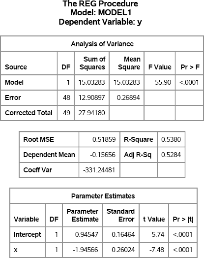
Figure 11.1 indicates that the simulated response, y, was generated according to the regression model. The RMSE is close to 0.5, which is the standard deviation of the random error term, and the parameter estimates are close to the population values of 1 and –2.
Notice that the x variable is randomly generated for this simulation. You could also have used uniformly spaced points (x=i) or normally distributed values, depending on the scenario that you are simulating.
How you generate the x variable depends on what you are trying to do:
- If you intend for x to be a fixed effect, the values of x should be generated (or read from a data set) one time at the beginning of the simulation. For each sample, the model for the response is computed by using the same values of x.
- If you think of x as a random effect, then the values of x should be simulated for each sample in the simulation.
If you are just generating some “quick and dirty” data to use to test some algorithm, then it might not matter which option you choose.
The next sections assume that you want to simulate a fixed effect. Consequently, you should generate values for the explanatory variable one time and retain those values during the simulation.
11.3.1.1 Using Arrays to Hold Explanatory Variables
One way to simulate a fixed effect is to use an array of length N. For each simulated sample, the same values of x are used to compute y.
/* Simulate multiple samples from a regression model */
/* Technique 1: Put explanatory variables into arrays */
%let N = 50;                           /* size of each sample      */
%let NumSamples = 100;                 /* number of samples        */
data RegSim1(keep= SampleID x y);
array xx{&N} _temporary_;              /* do not output the array  */
call streaminit(1);
do i = 1 to &N;                        /* create x values one time */
   xx{i} = rand(“Uniform”);
end;

do SampleID = 1 to &NumSamples;
   do i = 1 to &N;
      x = xx{i};                 /* use same values for each sample */
      y = 1 - 2*x + rand(“Normal”, 0, 0.5);  /* params are 1 and -2 */
      output;
   end;
end;
run;
This technique is also useful for simulating time series (see Chapter 13) because you can easily formulate models that use lagged values of the x variable. A minor drawback of this technique is that you need an array to store each explanatory variable. If you are generating a large number of variables, you might find it convenient to use a two-dimensional DATA step array.
11.3.1.2 Changing the Order of Loops
An alternative way to simulate a fixed effect is to reverse the usual order of the DO loops. The following example has an outer loop over observations and an inner loop for each sample:
/* Technique 2: Put simulation loop inside loop over observations */
data RegSim2(keep= SampleID i x y);
call streaminit(1);

do i = 1 to &N;
   x = rand(“Uniform”);          /* use this value NumSamples times */
   eta = 1 - 2*x;                /* parameters are 1 and -2         */
   do SampleID = 1 to &NumSamples;
      y = eta + rand(“Normal”, 0, 0.5);
      output;
   end;
end;
run;

proc sort data=RegSim2;
   by SampleID i;
run;
For this method, you must sort by the SampleID variable prior to running a BY-group analysis. Sorting by the observation number (the i variable) is not always necessary, but it is helpful to know that each simulated sample contains the observations in the same order. For time series data, sorting by both variables is required.
No matter which method you use to simulate the data, you can use the techniques that are described in Chapter 5, “Using Simulation to Evaluate Statistical Techniques,” to analyze the data. The following analysis examines the distributions of the parameter estimates:
proc reg data=RegSim2 outest=OutEst NOPRINT;
   by SampleID;
   model y = x;
quit;

ods graphics on;
proc corr data=OutEst noprob plots=scatter(alpha=.05 .1 .25 .50);
   label x=“Estimated Coefficient of x”
         Intercept=“Estimated Intercept”;
   var Intercept x;
   ods exclude VarInformation;
run;
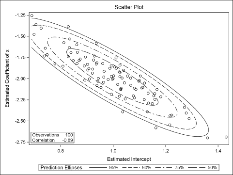
Figure 11.2 summarizes the approximate sampling distribution (ASD) of each parameter estimate. The output also shows that the estimates are strongly correlated with each other. The sample means for the parameter estimates (the Monte Carlo estimates) are extremely close to (1, –2), which are the population parameters. The Pearson correlation for the parameter estimates is about –0.89. These two facts are shown graphically in Figure 11.3, which shows a scatter plot of the parameter estimates along with probability contours for a bivariate normal distribution.
Figure 11.2 Approximate Sampling Distribution of Parameter Estimates
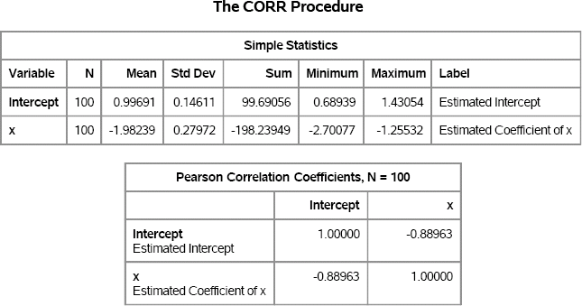
Figure 11.3 ASD of Parameter Estimates, N = 100
Exercise 11.1: Compare the computational efficiency of the “array method” (Section 11.3.1.1) and the “reverse loops and sort method.” Use 10,000 samples. Which technique is faster? Why?
Exercise 11.2: The OutEst data set also contains estimates for the RMSE for each simulated set of data. Use PROC UNIVARIATE to analyze the _RMSE_ variable. What is the Monte Carlo estimate for the RMSE? What is a 90% confidence interval? Test whether the ASD is normally distributed.
11.3.2 A Linear Model Based on Real Data
The previous section generated random values for the explanatory variable. This section describes ways to incorporate a model of real data into a simulation.
The “Getting Started” section for the SAS documentation on the REG procedure in the SAS/STAT User's Guide describes a regression analysis of weight as a function of height for 19 students. The following SAS statements reproduce two tables in the analysis:
ods graphics off;
proc reg data=Sashelp.Class;
   model Weight = Height;
   ods select FitStatistics ParameterEstimates;
quit;
Figure 11.4 Fit Statistics and Parameter Estimates for a Linear Model
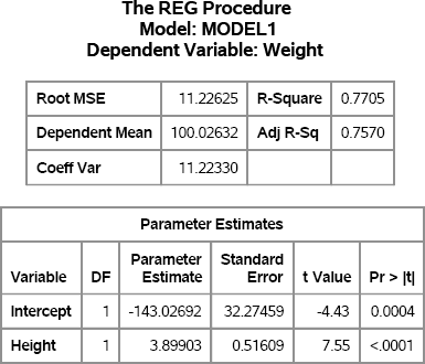
If you assume that the response variable, Weight, can be predicted by a linear function of Height, then the regression model that best fits the data is approximately
Weight = –143 + 3.9 × Height
The RMSE for the model is 11.23, so that value can be used for the standard deviation of an error term: ∊ ~ N(0, 11.23). The following sections describe several ways to simulate these data.
11.3.2.1 Using the Sample Data
The first approach uses the exact student heights for the simulation, but uses the regression model to simulate new responses (weights). You can imagine the simulated sample to be a matched cohort: You find 19 “new students” in the population that have exactly the same heights as the original students, and you “measure” their weights. The following DATA step reads in the original heights and simulates the weights:
data StudentData(keep= Height Weight);
call streaminit(1);
set Sashelp.Class;           /* implicit loop over observations     */
b0 = -143; b1 = 3.9;         /* parameter estimates from regression */
rmse =11.23;                 /* estimate of scale of error term     */
Weight = b0 + b1*Height + rand(“Normal”, 0, rmse);
run;
Notice that the linear expression b0 + b1*Height computes the predicted values of the regression. Consequently, an alternative but equivalent approach is to output the predicted values from PROC REG when you run the analysis. You can then generate new responses by adding a random term to the predicted value. An advantage to this approach is that you do not need to specify the regression coefficients explicitly.
Exercise 11.3: Use the P= option in the OUTPUT statement of the REG procedure to output the predicted values. Simulate new responses by adding a random error to each predicted value.
11.3.2.2 Simulations That Use the Sample Data
To generate multiple samples from the student data, add a DO loop to the programs in the previous section. The following DATA step reads the original Sashelp.Class data and simulates NumSamples values of the Weight variable for each observation in the data set. The Weight variable is simulated by using the regression model for the observed data.
/* duplicate data by using sequential access followed by a sort     */
%let NumSamples = 100;              /* number of samples            */
data StudentSim(drop= b0 b1 rmse);
b0 = -143; b1 = 3.9; rmse =11.23;   /* parameter estimates          */
call streaminit(1);
set Sashelp.Class;                  /* implicit loop over obs       */
i = _N_;
eta = b0 + b1*Height;               /* linear predictor for student */
do SampleID = 1 to &NumSamples;
   Weight = eta + rand(“Normal”, 0, rmse);
   output;
end;
run;

proc sort data=StudentSim;
   by SampleID i;
run;
You can avoid the inverted loops and the subsequent sorting if you use the POINT= option in the SET statement to randomly access observations. If you use this approach, then be sure to use the STOP statement after both loops have completed in order to prevent an infinite loop. The DATA step does not detect an end-of-file condition when you use random access, so you must explicitly stop the processing of data.
/* Alternative: simulate weights by using random access and no sort */
data StudentSim2(drop= b0 b1 rmse);
b0 = -143; b1 = 3.9; rmse = 11.23;  /* parameter estimates          */
call streaminit(1);
do SampleID = 1 to &NumSamples;
   do i = 1 to NObs;                /* NObs defined at compile time */
      set Sashelp.Class point=i nobs=NObs          /* random access */
      eta = b0 + b1*Height; /* linear predictor for student         */
      Weight = eta + rand(“Normal”, 0, rmse);
      output;
   end;
end;
STOP;     /* IMPORTANT: Use STOP with POINT= option in the SET stmt */
run;
Exercise 11.4: Call PROC REG on the StudentSim data, and use SampleID as a BY-group variable in order to generate the ASD of the regression coefficients.
Exercise 11.5: The second DATA step in this section reads the Sashelp.Class multiple times. Use the technique in Section 11.3.1.1 to read the Height variable into an array and access the array when building the linear model. Use a macro variable to hold the number of observations in the data set.
Exercise 11.6: The Sashelp.Cars data set has 428 observations. Generate 10,000 copies of the data by using each of the two techniques in this section. Compare the performance of the two methods. Which is faster?
11.3.2.3 Simulating Data from Regression Models in SAS/IML Software
You can use the SAS/IML language to simulate data from regression models. Because the SAS/IML language supports matrix and vector computations, the model is represented by the matrix equation Y = Xβ + ∊ where X is an N × p design matrix, β is a p-dimensional vector of regression parameters, and ∊ is an N-dimensional random vector such that each element is independently chosen from N(0, σ).
In order to include an intercept term in the model, the first column of X is a column of 1s. The model Yi = β0 + β1Xi + ∊i, for i = 1,…, N can be rewritten in vector notation as Yi = [1 Xi]β + ∊i, where β = (β0 β1)′.
The following SAS/IML program defines β = (–143 3.9)′ and forms the linear predictor:
proc iml;
call randseed(1);
beta = {-143, 3.9}; rmse = 11.23;

use Sashelp.Class NOBS N;               /* N = sample size         */
read all var {Height} into X1;          /* read data               */
close Sashelp.Class;

X = j(N,1,1) || X1;                     /* add intercept column    */
eta = X*beta;                           /* linear predictor        */
There are several ways to simulate the response variable. If you are going to analyze the simulated data in the SAS/IML language, then you can just loop over the number of simulations, as follows:
eps = j(N, 1);                           /* allocate N × 1 vector   */
do i = 1 to &NumSamples;
   call randgen(eps, “Normal”, 0, rmse); /* fill with random normal */
   Weight = eta + eps;                   /* one simulated response  */
   /* conduct further analysis */
end;
On the other hand, if you intend to write the data to a SAS data set for analysis by one of the regression procedures, you might want to generate all of the simulated data in “long” format, as follows:
eps = j(N * &NumSamples, 1);             /* allocate long vector    */
call randgen(eps, “Normal”, 0, rmse);    /* fill with random normal */
Wt = repeat(eta, &NumSamples) + eps;     /* simulate all responses  */
ID = repeat( T(1:&NumSamples), 1, N );   /* 1,1,1,…,2,2,2,…         */
Ht = repeat( X1, &NumSamples );
create SimReg var {ID Ht Wt};  append;  close SimReg; /* write data */
Exercise 11.7: Use PROC REG and a BY statement to analyze the simulated data. Compute the ASD for the parameter estimates.
11.3.2.4 Modeling the Data
Suppose that you do not have access to the original data, but that you are told that Figure 11.4 is the result of a regression on 19 students with mean height of 62.3 inches and standard deviation of 5.13 inches. If you assume that the heights are normally distributed, the following example creates simulated data with 19 observations. The heights and weights are not the same as for the original study, but are for a new set of 19 simulated students.
/* Original data not available. Simulate from summary statistics.   */
data StudentModel(keep= Height Weight);
call streaminit(1);
b0 = -143; b1 = 3.9;         /* parameter estimates from regression */
rmse =11.23;                 /* estimate of scale of error term     */
do i = 1 to 19;
   Height = rand(“Normal”, 62.3, 5.13);  /* Height is random normal */
   Weight = b0 + b1*Height + rand(“Normal”, 0, rmse);
   output;
end;
run;
The parameter estimates from the regression analysis are used to simulate a new data set with similar characteristics. The distribution of heights is modeled by a normal distribution.
This example shows a common technique in simulation: using parameter estimates as parameters. This approach is not perfect—for example, the Monte Carlo estimates are centered on the estimates instead of on the parameters—but because the parameter values are unknown, this is often the best that you can achieve.
An advantage to this approach is that you can use it to generate samples that are a different size than the original data sample. For example, you can change the upper bound for the DO loop from 19 to 50 to simulate heights and weights in a class that contains 50 students.
Exercise 11.8: Use the modeling approach to generate 1,000 samples of student heights and weights. For each sample, generate 19 “new” students with heights that are normally distributed. Analyze the distribution of the parameter estimates.
11.3.3 A Linear Model with a Single Classification Variable
The SAS documentation on the ANOVA procedure in the SAS/STAT User's Guide shows a “Getting Started” example of a one-way analysis of variance for a balanced design. In the example, the response variable depends on a classification variable that has six levels. There are five observations for each level. The assumed model is
Yij = μ + αi + ∊ij
where i = 1,…, 6 enumerates the treatment levels, ∊ij ~ N(0, σj), and j = 1,…, 5 enumerates the observations in each treatment group.
Assume that the overall mean is 20 and that the effect of the six treatment levels are 9, –6, –6, 4, 0, and 0. Assume that the corresponding standard deviations are 6, 2, 4, 4, 1, and 2. (These values are loosely based on an experiment that is described in the PROC ANOVA documentation.) The following DATA step simulates data from this balanced design:
data AnovaData(keep=Treatment Y);
call streaminit(1);
grandmean = 20;
array effect{6} _temporary_ (9 –6 –6 4 0 0);
array std{6}    _temporary_ (6  2  4 4 1 2);
do i = 1 to dim(effect);       /* number of treatment levels        */
   Treatment = i;
   do j = 1 to 5;              /* number of obs per treatment level */
      Y = grandmean + effect{i} + rand(“Normal”, 0, std{i});
      output;
   end;
end;
run;
The AnovaData data set contains simulated data from the regression model. You can call PROC ANOVA to analyze the simulated data, as follows. Figure 11.5 shows the results.
proc ANOVA data=AnovaData;
   class Treatment;
   model Y = Treatment;
   ods exclude ClassLevels NObs;
run;
Figure 11.5 ANOVA Analysis of Simulated Data
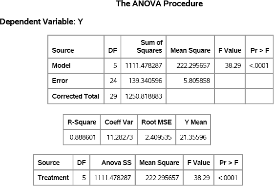
Each statistic in Figure 11.5 has a sampling distribution. Recall from Chapter 5 that you can simulate a sampling distribution by adding an additional DO loop to the DATA statement, such as
do SampleID = 1 to &NumSamples; /* simulation loop */
   …
end;
and by using a BY SampleID statement in the call to PROC ANOVA.
You can also simulate the regression data in SAS/IML software. Whereas the typical DATA step technique is to generate two columns of data (Treatment and Y), the preferred technique in the SAS/IML language is to construct a 6 × 5 matrix where each row represents a sample for a treatment level, as shown in the following program:
proc iml;
call randseed(1);
grandmean = 20;
effect = {9 -6 -6 4 0 0};
std    = {6  2  4 4 1 2};
N = 5;

/* each row of Y is a treatment */
Y = j(ncol(effect),N,.);  /* allocate matrix; fill with missing values */
ei = j(1,N);

do i = 1 to ncol(effect);
   call randgen(ei, “Normal”, 0, std[i]);
   Y[i,] = grandmean + effect[i] + ei;
end;
Exercise 11.9: Choose a statistic in the FitStatistics table in Figure 11.5, such as the R-square statistic, the coefficient of variation, or the RMSE. Use PROC ANOVA and the techniques from Chapter 5 to investigate the ASD for these statistics.
Exercise 11.10: In an unbalanced design, the number of observations is not constant among treatment groups. Suppose that the experiment uses sample sizes of 5, 10, 10, 12, 6, and 8 for the treatment groups.
- Write a DATA set that simulates data with these properties.
- Modify the SAS/IML program to simulate these data. One approach is to construct a 6 × K matrix, where K is the maximum sample size in the treatment groups, and use missing values to represent elements that are not part of the design.
11.3.4 A Linear Model with Classification and Continuous Variables
Sometimes you need a quick and easy way to simulate data from a regression model with many classification variables, many continuous variables, and a response variable. Suppose that you want to generate a predetermined number of continuous and classification variables, and you want each classification variable to have L levels. The following DATA step simulates (uncorrelated) data with these properties:
%let nCont = 4;              /* number of contin vars               */
%let nClas = 2;              /* number of class vars                */
%let nLevels = 3;            /* number of levels for each class var */
%let N = 100;
/* Simulate GLM data with continuous and class variables */
data GLMData(drop=i j);
array x{&nCont} x1-x&nCont;
array c{&nClas} c1-c&nClas;
call streaminit(1);

/* simulate the model */
do i = 1 to &N;
   do j = 1 to &nCont;               /* continuous vars for i_th obs */
      x{j} = rand(“Uniform”);        /* uncorrelated uniform         */
   end;
   do j = 1 to &nClas;               /* class vars for i_th obs      */
      c{j} = ceil(&nLevels*rand(“Uniform”));     /* discrete uniform */
   end;
   /* specify regression coefficients and magnitude of error term */
   y = 2*x{1} - 3*x{&nCont} + c{1} + rand(“Normal”);
   output;
end;
run;
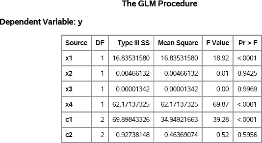
In this model, all continuous variables are uniformly distributed. Furthermore, the discrete levels of the classification variables are also uniformly distributed. The response variable in the example does not depend on all of the explanatory variables. It depends only on the first and last continuous variables and on the first classification variable. Consequently, if you analyze the simulated model, then there should be only three regression coefficients that are significant. The following statements use PROC GLM to analyze the data. The Type III sums of squares are shown in Figure 11.6. The three variables that were used to construct the response variable have p-values that are less than 0.0001.
proc glm data=GLMData;
   class c1-c&nClas;
   model y = x1-x&nCont c1-c&nClas / SS3;
   ods select ModelANOVA;
quit;
Figure 11.6 GLM Analysis of Simulated Data
Exercise 11.11: In the simulated data, each classification variable contains three levels. Modify the DATA step to simulate three classification variables for which the number of levels are 2, 3, and 4, respectively.
11.4 The Power of a Regression Test
This section presents a case study that shows how to use simulation to investigate the power of a statistical test.
When examining regression models, it is common to ask whether the coefficient of an explanatory effect is significantly different from zero. The TEST statement in the REG procedure can be used to test whether a regression coefficient is zero, given the data.
To demonstrate the TEST statement, the following statements simulate a single sample of data for a regression model for which the coefficient of the z variable is exactly zero. The results are shown in Figure 11.7.
data Reg1(drop=i);
call streaminit(1);
do i = 1 to &N;
   x = rand(“Normal”);
   z = rand(“Normal”);
   y = 1 + 1*x + 0*z + rand(“Normal”);      /* eps ~ N(0,1) */
   output;
end;
run;

proc reg data=Reg1;
   model y = x z;
   z0: test z=0;
   ods select TestANOVA;
quit;
Figure 11.7 Test whether a Regression Parameter Is Zero
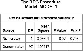
The TestANOVA table, which is shown in Figure 11.7, shows the result of an F test for the null hypothesis that the coefficient of the z variable is zero. The p-value for the F test is large, which indicates that there is little evidence to reject the null hypothesis. This result is expected, because the data were simulated so that the null hypothesis is true.
You can conduct a simulation that examines the power of the TEST statement to detect small (but nonzero) values of the regression coefficient. The F test assumes that the error term of the regression model is normally distributed and is homoscedastic. But how does the F test behave if these assumptions are violated?
A simulation that is presented in Greene (2000, Ch. 15) examines this question. Greene examines three different error distributions for the error term in the regression model:
- The error term is normally distributed. This is the usual assumption that, if true, implies that the statistic in the TestANOVA table follows an F distribution.
- The error term follows a t distribution with 5 degrees of freedom. This distribution is similar to a normal distribution, but has fatter tails.
- The error term is heteroscedastic. Greene (2000) uses a normal distribution in which the standard deviation is exp(0.2x), which depends on the values of the x variable. Greene (2000, p.617)comments that “the statistic is entirely wrong if the disturbances are heteroscedastic.”
The design of Greene's simulation is to draw 50 uncorrelated observations of two variables, x and z, from N(0,1). For each observation, compute the true model as ηi = 1 + xi, + γzi, and compute yi = ηi + ∊i for each of the three kinds of error distributions. Repeat this simulation for a sequence of γ values in the range [0, 1]. The following DATA step simulates data according to this scheme:
%let N = 50;
%let NumSamples = 1000;                    /* number of samples    */
data RegSim(drop= i eta sx);
call streaminit(1);
do i = 1 to &N;
   x = rand(“Normal”); z = rand(“Normal”);
   sx = exp(x/5);                          /* StdDev for model 3   */
   do gamma = 0 to 1 by 0.1;
      eta = 1 + 1*x + gamma*z;             /* linear predictor     */
      do SampleID = 1 to &NumSamples;
         /* Model 1: e ~ N(0,1)         */
         /* Model 2: e ~ t(5)           */
         /* Model 3: e ~ N(0, exp(x/5)) */
         Type = 1   y = eta + rand(“Normal”);         output;
         Type = 2   y = eta + rand(“T”, 5);           output;
         Type = 3   y = eta + rand(“Normal”, 0, sx);  output;
      end;
   end;                                    /* end gamma loop        */
end;                                       /* end observation loop  */
run;

proc sort data=RegSim out=Sim;
   by Type gamma SampleID;
run;
As described in Section 11.3.1.2, the order of the DO loops in this simulation requires that you sort the data prior to running the regression analysis.
The following PROC REG statement analyzes each set of simulated data for each kind of error distribution (Type), for each value of the regression coefficient (gamma), and for each of 1,000 samples (SampleID):
/* Turn off output when calling PROC for simulation */
%ODSOff
proc reg data=Sim;
   by Type gamma SampleID;
   model y = x z;
   test z=0;
   ods output TestANOVA=TestAnova;
quit;
%ODSOn
The following statements count the number of times that the null hypothesis (γ = 0) was rejected for each kind of error distribution for each value of γ:
/* 3. Construct an indicator variable for observations that reject H0 */
data Results;
   set TestANOVA(where=(Source=“Numerator”));
   Reject = (ProbF <= 0.05);                  /* indicator variable */
run;

/* count number of times H0 was rejected */
proc freq data=Results noprint;
   by Type gamma;
   tables Reject / nocum out=Signif(where=(reject=1));
run;

data Signif;
   set Signif;
   proportion = percent / 100;      /* convert percent to proportion */
run;
You can plot the proportion of times that the null hypothesis is rejected. For γ > 0, the test commits a Type II error if it fails to reject the null hypothesis. The results are shown in Figure 11.8:
proc format;
   value ErrType 1=“e ~ N(0,1)” 2=“e ~ t(5)” 3=“e ~ Hetero”;
run;

title “Power of F Test for gamma=0”;
title2 “N = &N”;
proc sgplot data=Signif;
   format Type ErrType.;
   series x=gamma y=proportion / group=Type;
   yaxis min=0 max=1 label=“Power (1 - P[Type II Error])” grid;
   xaxis label=“Gamma” grid;
   keylegend / across=1 location=inside position=topleft;
run;
Figure 11.8 Power Curves for Testing whether a Coefficient Is Zero
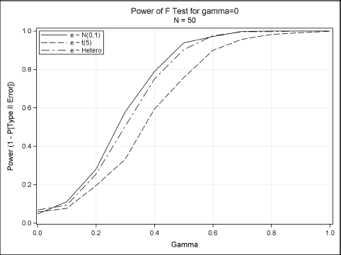
Figure 11.8 shows how the power curve for the F test varies for the three error distributions. Greene concludes that “it appears that the presence of heteroscedasticity [does not] degrade the power of the statistic. But the different distributional assumption does.”
Exercise 11.12: Use DATA step arrays, as described in Section 11.3.1.1, to rewrite the DATA step so that no sort is required.
Exercise 11.13: Set γ = 0 in the regression model. When the error term follows an N(0,1) distribution, the F statistic in the TestANOVA table follows an F2,N–2 distribution. Examine the sampling distribution for the other choices of the error distribution. Does the F statistic appear to be sensitive to the shape of the error distribution?
11.5 Linear Models with Interaction and Polynomial Effects
Previous sections have simulated data from regression models with main effects. This section shows how to simulate data with interaction and polynomial effects.
11.5.1 Polynomial Effects
It is easy to simulate data that contain a polynomial effect. For example, for the regression model
Yi = 1 – 2Xi + 3Xi2 + ∊i
you can use the following DATA step syntax:
y = 1 - 2*x + 3*x*x + eps; /* include quadratic effect */
For multivariate polynomials, you can create interactions between two continuous variables simply by multiplying the variables together. In the SAS/IML language, use the elementwise multiplication operator (#) to multiply the elements of two vectors.
Exercise 11.14: Simulate 1,000 observations from the two-variable regression model Yi = 1 – 2Xi + 3Zi + Xi2 – XiZi + ∊i, where ∊ ~ N(0,1). Run the GLM procedure to verify that the simulated data are from the specified model.
11.5.2 Design Matrices
Many interesting models include interactions between variables, and it is not always easy to use the DATA step to specify the interactions. An alternative approach is to use SAS/STAT procedures to create a design matrix for the effects. A design matrix is a unified way to incorporate classification variables, continuous variables, and interactions. You can then read the design matrix into PROC IML and simulate the data by using the matrix model Y = Xβ + ∊. Here X is an N × p design matrix, β is a p-dimensional vector of regression parameters, and ∊ is an N-dimensional random vector with zero mean.
There are various parameterizations that you can use to create dummy variables from classification variables. The most common parameterization is the GLM parameterization (also called a singular parameterization), which you can generate by using the GLMMOD procedure. The LOGISTIC procedure supports alternate parameterizations. You can create design matrices for models that include continuous variables, but the examples in this section only include classification variables and their interactions.
11.5.2.1 Design Matrices with GLM Parameterization
Suppose that you want to simulate data for a study that has two classification variables. The Drug variable contains three levels and the Disease variable contains two levels. Furthermore, you want the mean response to depend on the explanatory variables according to Table 11.1.
Table 11.1 Mean Response for Joint Levels
| Disease | ||
| Drug | 1 | 2 |
| 1 | 10 | 0 |
| 2 | 15 | -5 |
| 3 | 20 | -10 |
The following DATA step creates a balanced design matrix with five repeated measurements for each joint level of Drug and Disease. The value of the response variable (y) is arbitrary and unimportant, because the sole purpose of this DATA step is to generate a design matrix for the explanatory variables.
data Interactions;
y = 0;                                  /* the value of y does not matter */
do drug = 1 to 3;
   do disease = 1 to 2;
      do subject = 1 to 5;
         output;
      end;
   end;
end;
run;
You can use the GLMMOD procedure to generate a design matrix from the Interactions data set. The GLMMOD procedure enables you to specify the effects (including interaction terms), and it generates a design matrix that corresponds to the model. For example, the following statements generate a design matrix for a model for which the response variable depends on Drug, Disease, and their interaction:
proc glmmod data=Interactions noprint
            outparm=Parm outdesign=Design(drop=y);          /* DROP y */
   class drug disease;
   model y = drug | disease;
run;
The GLMMOD procedure creates two data sets. The Parm data set maps the 12 columns of the design matrix to the corresponding variable names and levels. The Design data set contains the design matrix. Notice that the DROP= data set option is used to prevent the y variable from appearing in the Design data. The columns of the Design data set are named Col1–Col12.
You can construct a parameter vector of regression coefficients and use matrix multiplication in PROC IML to form the linear model and to add a random error term, as shown in the following statements:
proc iml;
call randseed(1);
use Design;
read all var _NUM_ into X;
close Design;

/* Intcpt |--Drug--|Disease|-----Interactions-----| */
beta = {0, 0, 0, 0,  0, 0,  10, 0, 15, -5, 20, -10};
eps = j(nrow(X),1);                        /* allocate error vector */
call randgen(eps, “Normal”);
y = X*beta + eps;

create Y var{y};   append;   close Y;      /* write to data set */
In this example, the design matrix is rank 6, which means that there are six linearly independent columns. Consequently, there are many equivalent ways to specify the linear model that relates the design matrix to y. The approach used in the program makes it clear that Table 11.1 describes the expected value of the response for each joint level of the Drug and Disease variables.
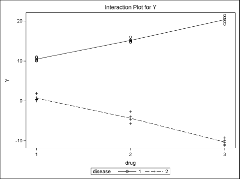
To check that the simulated responses are correct, run the GLM procedure and graph the observed and predicted values for each level of the classification variables, as shown in the following statements:
data D;
   merge Y Interactions(drop=y);
run;

ods graphics on;
proc glm data=D;
   class drug disease;
   model y = drug | disease / solution p;
run;
Figure 11.9 shows that the predicted values for Disease=1 are approximately 10, 15, and 20. The predicted values for Disease=2 are approximately 0, –5, and –10. This shows close agreement with Table 11.1.
Because the design matrix is singular, the parameter estimates found by PROC GLM might not be the same as the parameter values that were used to construct the data. However, the predicted values (which are not shown) are independent of the parameterization.
Figure 11.9 Graph of Observed and Predicted Values
11.5.2.2 Design Matrices for Alternative Parameterizations
The GLMMOD procedure creates a singular design matrix, which means that the parameter estimates are not unique. Several SAS procedures support nonsingular parameterizations for classification effects. Two popular alternative parameterizations are the “effect” and “reference” parameterizations. You can generate design matrices for these and other parameterizations by using the LOGISTIC procedure.
The PROC LOGISTIC statement supports the OUTDESIGN= and OUTDESIGNONLY options. You can use these options to generate a design matrix without actually fitting a logistic model. Because no model is fit, you can set the values of the response variable to be a constant value, such as 0. Notice that the Interactions data set (which was created in Section 11.5.2.1) has a constant value for Y. Consequently, the following PROC LOGISTIC statement generates a design matrix by using the reference parameterization. The reference parameterization is specified by the PARAM=REFERENCE option in the CLASS statement.
proc logistic data=Interactions
              outdesignonly outdesign=DesignRef(drop=y);
   class drug disease / param=reference;
   model y = drug | disease;
run;
The PROC LOGISTIC statements write the design matrix to the DesignRef data set. The design matrix has only six columns, whereas the design matrix that is created by PROC GLMMOD has 12 columns. For details about nonsingular parameterizations and how to specify them, see the section “Parameterization of Model Effects” in the chapter “Shared Concepts and Topics” in the SAS/STAT User's Guide.
11.6 Outliers and Robust Regression Models
A common simulation task is to assess the robustness of statistical methods in the presence of outliers. In a regression model, the word outlier means an outlier for the response variable. This is an observation for which the observed response is much different than would be predicted by a robust fit of the data.
Observations can also have highly unusual values for the explanatory variables. These observations are called high-leverage points because they can unduly influence parameter estimates for an ordinary least squares fit.
This section describes how to simulate regression data with outliers and high-leverage points.
11.6.1 Simulating Outliers
This section describes how to generate extreme values (outliers) for a response variable. For simplicity, suppose that you want to simulate data for a univariate regression model that is given by
Yi = 1 – 2Xi + ∊i
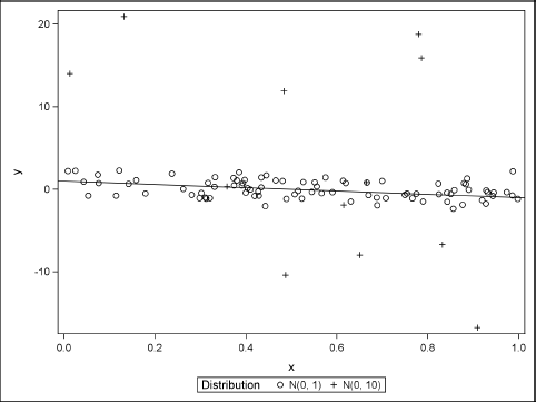
where ∊i follows a contaminated normal distribution as described in Section 7.5.2. (In general, you can choose any long-tailed distribution for ∊.) For concreteness, assume that ∊i follows an N(0, 1) distribution 90% of the time and an N(0, 10) distribution 10% of the time. The following DATA step simulates one sample:
%let N = 100;                           /* size of each sample       */
data RegOutliers(keep=x y Contaminated);
array xx{&N} _temporary_;
p = 0.1;                                /* prob of contamination     */
call streaminit(1);
/* simulate fixed effects */
do i = 1 to &N;
   xx{i} = rand(“Uniform”);
end;
/* simulate regression model */
do i = 1 to &N;
   x = xx{i};
   Contaminated = rand(“Bernoulli”, p);
   if Contaminated then eps = rand(“Normal”, 0, 10);
   else                 eps = rand(“Normal”, 0, 1);
   y = 1 - 2*x + eps;                   /* parameters are 1 and -2 */
   output;
end;
run;
You can use PROC SGPLOT to plot the data and the model. Figure 11.10 shows that most of the simulated data fall close to the line y = 1 – 2x. The line is displayed by using the LINEPARM statement. Nine points are outliers.
proc format;
   value Contam 0=“N(0, 1)” 1=“N(0, 10)”;
run;

proc sgplot data=RegOutliers(rename=(Contaminated=Distribution));
   format Distribution Contam.;
   scatter x=x y=y / group=Distribution;
   lineparm x=0 y=1 slope=-2;      /* requires SAS 9.3 */
run;
Figure 11.10 Graph of Simulated Data with 10% Contaminated Errors
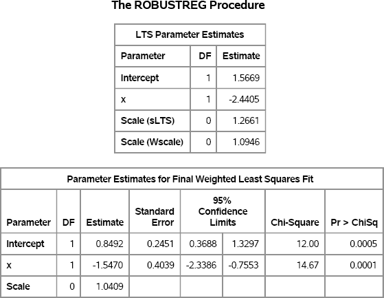
If you exclude the points for which Contaminated=0, then the parameter estimates are close to the parameter values. Of course, in practice you do not know which observations are contaminated. However, you can use the ROBUSTREG procedure to produce a robust regression estimate of the parameters. The following statements use the least trimmed squares (LTS) method to identify outliers. The FWLS option displays the final weighted least squares (FWLS) estimates (shown in Figure 11.11), which are the OLS estimates after the outliers are set to have zero weight.
proc robustreg data=RegOutliers method=lts FWLS;
   model y = x;
   ods select LTSEstimates ParameterEstimatesF;
run;
For these simulated data, both the LTS estimates and the FWLS estimates are somewhat close to the parameter values. The two estimates are usually similar, but are computed in different ways. The LTS estimates are based on a subset of the data (by default, about 75%). The LTS estimates are used to determine which observations are outliers. The FWLS estimates are ordinary least squares estimates that exclude the outliers.
Figure 11.11 Robust Parameter Estimates
By using the technique in this section, you can simulate data that contain outliers for the response variable, and compare the parameter estimates that are computed by least-squares and robust regression algorithms.
Exercise 11.15: Use PROC REG to run a regression analysis on the RegOutliers data. Include the CLB option in the MODEL statement to compute 95% confidence intervals for the parameters. Do the confidence intervals include the parameters for this example?
11.6.2 Simulating High-Leverage Points
Extreme values in the space of the explanatory variables are called high-leverage points. To simulate data that contain high-leverage points and outliers, do the following:
- Generate a matrix of observations, X, from a multivariate contaminated normal distribution, as described in Section 8.5.1.
- Generate error terms from a univariate contaminated normal distribution.
- Form the regression model as Y = Xβ + ∊.
This algorithm is implemented in the following SAS/IML program. The explanatory variables are simulated from a multivariate normal distribution with 15% contamination. The error term is univariate normal with 25% contamination. In the simulation, the intercept term is assigned separately; the X matrix does not include a column of ones for the intercept. It is often more efficient not to waste space and computations on that scalar quantity.
/* simulate outliers and high-leverage points for regression data   */
%let N = 100;
proc iml;
call randseed(1);
mu = {0 0 0};                        /* means                       */
Cov = {10 3 -2, 3 6 1, -2 1 2};      /* covariance for X            */
kX = 25;                             /* contamination factor for  X */
pX = 0.15;                           /* prob of contamination for X */
kY = 10;                             /* contamination factor for  Y */
pY = 0.25;                           /* prob of contamination for Y */

/* simulate contaminated normal (mixture) distribution */
call randgen(N1, “Binomial”, 1-pX, &N); /* N1=num of uncontaminated */
X = j(&N, ncol(mu));
X[1:N1,] = RandNormal(N1, mu, Cov);        /* draw N1 from uncontam */
X[N1+1:&N,] = RandNormal(&N-N1, mu, kX*Cov); /* N-N1 from contam    */

/* simulate error term according to contaminated normal */
outlier = j(&N, 1);
call randgen(outlier, “Bernoulli”, pY);    /* choose outliers       */
eps = j(&N, 1);
call randgen(eps, “Normal”, 0, 1);         /* uncontaminated N(0,1) */
outlierIdx = loc(outlier);
if ncol(outlierIdx)>0 then                 /* if outliers…          */
   eps[outlierIdx] = kY * eps[outlierIdx]; /* set eps ~ N(0, kY)     */

/* generate Y according to regression model */
beta = {2, 1, -1};               /* params, not including intercept */
Y = 1 + X*beta + eps;
The vector Y is the response vector for the regression model. In order to estimate the parameters in the model, you need to use a robust regression algorithm that detects high-leverage points. The following statements write the data to a SAS data set and call the ROBUSTREG procedure with the LTS algorithm to analyze the data. The LEVERAGE option in the MODEL statement requests the computation of leverage diagnostics. Both outliers and high-leverage points are written to the Out data set by the LEVERAGE= option in the OUTPUT statement.
/* write SAS data set */
varNames = (‘x1’:‘x3’) || {“Y” “Outlier”};
output = X || Y || outlier;
create Robust from output[c=varNames]; append from output; close;
quit;

proc robustreg data=Robust method=LTS plots=RDPlot;
   model Y = x1-x3 / leverage;
   output out=Out outlier=RROutlier leverage=RRLeverage;
   ods select LTSEstimates DiagSummary RDPlot;
run;
Figure 11.12 Robust Parameter Estimates for Contaminated Data
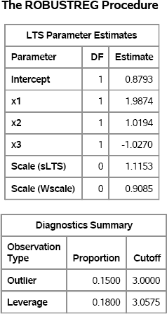
The parameter estimates are close to the parameter values. The “Diagnostics Summary” table reports how many outliers and high-leverage points were detected. For these simulated data, 15 (15% of the 100 observations) were classified as outliers and 18 points have high-leverage.
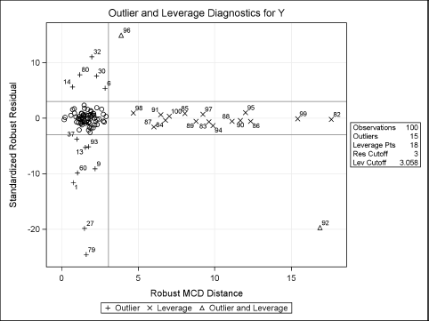
The classification of the observations is shown graphically in Figure 11.13. Points that are plotted outside of the horizontal lines at ±3 are classified as outliers. Points that are to the right of the vertical line at 3.0575 are classified as high-leverage points. Outliers and high-leverage points are marked by their observation numbers. The high-leverage points correspond to observations near the end of the data set. (Recall that the first N1 observations were drawn from an uncontaminated distribution.)
The indicator variables RROutlier and RRLeverage in the output data set identify which observations were classified as outliers and leverage points, respectively. You can compare these indicator variables with the simulated data.
Exercise 11.16: Use PROC FREQ to create a crosstabulation table that shows the relationship between the Outlier and RROutlier variables in the Out data set. The Outlier variable indicates how the observation was generated. Explain why there are observations with Outlier=1 that are not classified as outliers by the ROBUSTREG procedure.
Figure 11.13 Outliers and High-Leverage Points
11.7 References
Greene, W. H. (2000), Econometric Analysis, 4th Edition, Upper Saddle River, NJ: Prentice-Hall.