Chapter 9

Advanced Simulation of Multivariate Data

Contents

9.1 Overview of Advanced Multivariate Simulation

The previous chapter describes how to simulate data from commonly encountered multivariate distributions. This chapter describes how to simulate correlated data for more specialized distributions.

An interesting problem in multivariate simulation is the following. Suppose that you want to specify the marginal distribution of each of p variables and you also want to specify the correlations between variables. For example, you might want the first random variable to follow a gamma distribution, the second variable to be exponential, and the third to be normally distributed. Furthermore, you want to specify the correlations between the variables, such as ρ₁₂ = 0.1, ρ₁₃ = –0.2, and ρ₂₃ = 0.3.

In general, this is a difficult problem. To further complicate matters, there are some combinations of marginal distributions and correlations that cannot be mathematically satisfied. That is, when the marginal distributions hold, some correlations are impossible. However, if the specified correlations are feasible, then the copula technique might enable you to sample from a multivariate distribution with the given conditions. Copula techniques are heavily used in the fields of finance and econometrics.

Although it is common practice to separately model the marginal distribution and the correlation structure, you should think carefully about whether your model makes mathematical sense. As Schabenberger and Gotway (2005) write: “It may be tempting to combine models for mean and covariance structure that maybe should not be considered in the same breath. The resulting model may be vacuous.” In other words, a joint distribution function with the specified marginal distributions and covariance structure might not exist. Schabenberger and Gotway opine that it is “sloppy” to ask whether you can simulate behavior for which “no mechanism comes to mind that could generate this behavior.” Those who proceed in spite of these cautions might seek justification in George Box's famous quote, “All models are wrong, but some are useful.”

This chapter begins with a detailed description of how to simulate from two discrete distributions: the multivariate binary and multivariate ordinal distributions. You do not need to learn all of the details in order to use the SAS programs that simulate from these distributions. However, the literature is full of similar constructions, and the author hopes that a careful step-by-step description will help you understand how to simulate data from multivariate distributions that are not included in this book.

9.2 Generating Multivariate Binary Variates

Emrich and Piedmonte (1991) describe a straightforward algorithm for generating d binary variables, X₁, X₂, … , X_d, such that

• The probability of success, p_i, is specified for each Bernoulli variable, X_i, i = 1, … , d. The corresponding probabilities of failure are q_i = 1 – p_i.
• The Pearson correlation, corr(X_j, X_k) = δ_jk, is specified for each j = 1, … , d and k = i + 1, … , d. For convenience, let Δ be the specified correlation matrix.

As noted by Emrich and Piedmonte (1991), the correlation corr(X_j, X_k) for two binary variables is constrained by the expected values of X_j and X_k. Specifically, given p_j and p_k, the feasible correlation is in the range [L, U], where , .

The Emrich-Piedmonte algorithm consists of the following steps:

1. (Optional) Check the specified parameters to ensure that it is feasible to solve the problem.
2. For each j and k, solve the equation for ρ_jk, where Φ is the cumulative distribution function for the standard bivariate normal distribution and where z(.) is the quantile function for the univariate standard normal distribution. That is, given the desired correlation matrix, Δ, find an “intermediate” correlation matrix, R, with off-diagonal elements equal to ρ_jk.
3. Generate multivariate normal variates: (X₁, … , X_k) with mean 0 and correlation matrix R.
4. Generate binary variates: B_j = 1 when X_j < z(p_j); otherwise, B_j = 0.

The algorithm requires solving an equation in Step 2 that involves the bivariate normal cumulative distribution. You have to solve the equation d(d – 1)/2 times, which is computationally expensive, but you can use the solution to generate arbitrarily many binary variates. The algorithm has the advantage that it can handle arbitrary correlation structures. Other researchers (see Oman (2009) and references therein) have proposed faster algorithms to generate multivariate binary variables when the correlation structure is a particular special form, such as AR(1) correlation.

Because the equation in Step 2 is solved pairwise for each ρ_jk, the matrix R might not be positive definite.

9.2.1 Checking for Feasible Parameters

Step 1 of the algorithm is to check that the pairwise correlations and the marginal probabilities are consistent with each other. Given a pair of marginal probabilities, p_i and p_j, not every pairwise correlation in [–1, 1] can be achieved. The following SAS/IML function verifies that the correlations for the Emrich-Piedmonte algorithm are feasible:

proc iml;
/* Let X1, X2, … ,Xd be binary variables, let
    p = (p1, p2, … ,pd) the their expected values and let 
    Delta be the d × d matrix of correlations.
    This function returns 1 if p and Delta are feasible for binary 
    variables. The function also computes lower and upper bounds on the 
    correlations, and returns them in LBound and UBound, respectively */ 
start CheckMVBinaryParams(LBound, UBound, _p, Delta);
    p = rowvec(_p);    q = 1 – p;       /* make p a row vector */
    d = ncol(p);                        /* number of variables */

    /* 1. check range of Delta; make surep and Delta are feasible */
    PP = p`*p;    PQ = p`*q;
    QP = q`*p;    QQ = q`*q;
    A = -sqrt(PP/QQ); B = -sqrt(QQ/PP);  /* matrices */
    LBound = choose(A>B,A,B);            /* elementwise max(A or B) */
    LBound[loc(I(d))] = 1;               /* set diagonal to 1 */
    A = sqrt(PQ/QP); B= sqrt(QP/PQ);
    UBound = choose(A<B,A,B);            /* min(A or B) */
    UBound[loc(I(d))] = 1;               /* set diagonal to 1 */

    /* return 1 <==> specified means and correlations are feasible */
    return( all(Delta >= LBound) & all(Delta <= UBound) ); 
finish;

The implementation uses matrix arithmetic instead of DO loops to compute the bounds. The matrix PP contains products of the form p_j p_k, the matrix QQ contains products of the form q_j q_k, and so forth. The matrices A and B contain the square root of ratios of products, which are used to construct the upper and lower bounds for the elements of the correlation matrix.

9.2.2 Solving for the Intermediate Correlations

In SAS software, the PROBBNRM function computes the cumulative bivariate normal distribution. For an ordered pair (x, y), the PROBBNRM function returns the probability that an observation (X, Y) is less than or equal to (x, y), where X and Y are standard normal random variables with correlation ρ. You can use the QUANTILE function to compute the quantile of the normal distribution. Consequently, the following module evaluates the function in Step 2 of the algorithm. The parameters p_j, p_k, and δ_jk are passed in as global variables, where p_j is the probability of success for the j th binary variable, p_k is the probability of success for the k th binary variable, and δ_jk is the target correlation between the binary variables.

/* Objective: Find correlation, rho, that is zero of this function. 
   Global variables:
   pj = prob of success for binary var Xj 
   pk = prob of success for binary var Xk 
   djk = target correlation between Xj and Xk   */ 
start MVBFunc(rho) global(pj, pk, djk);
   Phi = probbnrm(quantile(“Normal”, pj), quantile(“Normal”, pk), rho);
   qj = 1-pj; qk = 1-pk;
   return( Phi - pj*pk - djk*sqrt(pj*qj*pk*qk) ); 
finish;

9.2.3 Simulating Multivariate Binary Variates

By using the modules that are defined in the preceding sections, you can write a function that generates multivariate binary variates with a given set of expected values and a specified correlation structure. If you are running SAS/IML 12.1 or later, then you can use the FROOT function to find the intermediate correlations. Prior to SAS/IML 12.1, you can use the Bisection module, which is included in Appendix A.

start RandMVBinary(N, p, Delta) global(pj, pk, djk);
    /* 1. Check parameters. Compute lower/upper bounds for all (j, k) */ 
    if ^CheckMVBinaryParams(LBound, UBound, p, Delta) then do;
      print “The specified correlation is invalid.” LBound Delta UBound;
      STOP;
    end;

    q = 1 - p;
    d = ncol(Delta);     /* number of variables */

    /* 2. Construct intermediate correlation matrix by solving the
        bivariate CDF (PROBBNRM) equation for each pair of vars */
    R = I(d); 
    do j = 1 to d-1; 
      do k = j+1 to d;
         pj=p[j]; pk=p[k]; djk = Delta[j, k];   /* set global vars */
         *R[j, k] = bisection(LBound[j, k], UBound[j, k]); /* pre-12.1 */ 
         R[j,k] = froot(“MVBFunc”, LBound[j, k]||UBound[j, k]);/* 12.1 */ 
         R[k, j] = R[j, k]; 
      end; 
    end;

    /* 3: Generate MV normal with mean 0 and covariance R */ 
    X = RandNormal(N, j(1, d, 0), R);
    /* 4: Obtain binary variable from normal quantile */ 
    do j = 1 to d;
       X[,j] = (X[,j] <= quantile(“Normal”, p[j])); /* convert to 0/1 */
    end;
    return (X);
finish;

The RANDMVBINARY function implements the Emrich-Piedmonte algorithm. Given a vector of probabilities, p, and a desired correlation matrix Delta, the RANDMVBINARY function returns an N × d matrix that contains zeros and ones. Each column of the returned matrix is a binary variate, and the sample mean and correlation of the simulated data should be close to the specified parameters, as shown in the following example:

call randseed(1234);
p = {0.25 0.75 0.5};         /* expected values of the X[j] */
Delta = { 1 -0.1 -0.25, 
         -0.1 1 0.25, 
         -0.25 0.25 1 };     /* correlations between the X[j] */
X = RandMVBinary(1000, p, Delta); 
/* compare sample estimates to parameters */ 
mean = mean(X); 
corr = corr(X);
print p, mean, Delta, corr[format=best6.];

Figure 9.1 Parameters and Sample Estimates from Simulated Binary Data

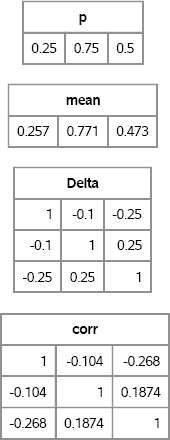
The matrix X contains 1,000 random draws from the multivariate binary distribution with the specified expected values and correlations. Figure 9.1 shows that the mean of each column is close to the expected value of the distribution. The sample correlation between columns is close to the specified correlations between variables.

9.3 Generating Multivariate Ordinal Variates

Simulating binary correlated variables is a particular case of the more general problem of simulating multivariate correlated ordinal variables. This section describes the algorithm of Kaiser, Träger, and Leisch (2011), which builds on the work of Demirtas (2006).

In particular, this section simulates data from a multivariate distribution with d > 2 ordinal variables, X₁, X₂, … , X_d. Assume that the j th variable has N_j values, 1, 2, … , N_j. Each random variable is defined by its probability mass function (PMF): P(X_j = i) = P_ij for i = 1, 2, … , N_j.

9.3.1 Overview of the Mean Mapping Method

The paper by Kaiser, Träger, and Leisch (2011) contains two algorithms. The algorithm presented here is called the “mean mapping method.” The algorithm generalizes the Emrich-Piedmonte method that is described in Section 9.2. The algorithm is as follows:

1. (Optional) Given marginal PMFs for the ordinal variables and a target correlation matrix, Δ, that describes their pairwise correlations, check that it is feasible to solve the problem. The feasibility of the problem is not checked in this book.
2. For each pair of ordinal variables, X_i and X_j, solve a complicated equation that involves the cumulative distribution function for the standard bivariate normal distribution. The solution to the equation gives a pairwise correlation, ρ_ij. Let R be the matrix with R_ij = ρ_ij.
3. Generate multivariate normal variables (Y₁, Y₂, … , Y_k) ~ MVN(O, R).
4. Use quantiles of the univariate standard normal distribution to convert Y_j to X_j.

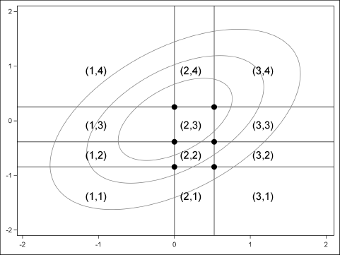
The general idea of the algorithm is shown in Figure 9.2. You generate multivariate normal data according to some correlation matrix, R. You can then use the probability of each marginal category to discretize the data. In the figure, normal bivariate points with coordinates in the lower left corner are assigned the value 1 for the first ordinal variable and the value 1 for the second variable. Points in the upper left corner are assigned 1 for the first ordinal variable and 4 for the second variable. Points near the origin are assigned to 1 or 2 for the first variable and 3 for the second, and so on.

Because of the discretization process, the correlation between the ordinal variables will usually be different from the correlation of the multivariate normal distribution from which the variables were generated. The purpose of Step 2 is to find the matrix R that gives rise to the desired correlation matrix, C.

Exercise 9.1: Let Z be an ordinal random variable with outcomes 1-4 and probability vector {0.2, 0.15, 0.25, 0.4}. Use the “Table” distribution (see Section 2.4.5) to simulate 10,000 observations from this distribution. Compute the sample mean and variance of the data.

Figure 9.2 Generate Correlated Ordinal Values from Bivariate Normal Data

9.3.2 Simulating Multivariate Ordinal Variates

This book's Web site contains a set of SAS/IML functions for simulating multivariate ordinal data. You can download and store the functions in a SAS/IML library, and use the LOAD statement to read the modules into the active PROC IML session, as follows:

/* Define and store the functions for random ordinal variables */ 
%include “C:<path>RandMVOrd.sas”;

proc iml;
load module=_all_;        /* load the modules */

To represent a multivariate ordinal distribution, you need to specify the marginal PMFs and the desired correlations between variables. One way to represent the PMFs is to store them as columns of a matrix, P. If you have d ordinal variables and the j th variable has N_j values, then P is an m × d matrix, where m = max_j N_j. You can use missing values to “pad” the matrix for variables that have a small number of values. This is the representation used by the modules in this section.

Let P be a SAS/IML matrix that specifies the PMFs for d ordinal variables. The following functions are used in this book:

• The ORDMEAN function, which returns the expected values for a set of ordinal random variables. The syntax is mean = OrdMean(P).
• The ORDVAR function, which returns the variance for a set of ordinal random variables. The syntax is var = OrdVar(P).
• The RANDMVORDINAL function, which generates N observations from a multivariate distribution of correlated ordinal variables. The syntax is X = RandMVOrd(N, P, Corr), where Corr is the d × d correlation matrix.

For example, the following matrix contains the PMFs of three ordinal variables. The first variable has two values and the PMF {0.25,0.75}; the last variable has four values and the PMF {0.20,0.15,0.25,0.40}. The ORDMEAN and ORDVAR functions are used to display the expected values and the variances of the three random variables:

    /* P1  P2   P3 */
P = {0.25 0.50 0.20 , 
     0.75 0.20 0.15 ,
      .   0.30 0.25 , 
      .    .   0.40 };

/* expected values and variance for each ordinal variable */ 
Expected = OrdMean(P) // OrdVar(P); 
varNames = “X1”:“X3”;
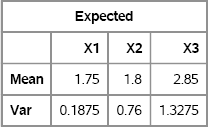
print Expected[r={“Mean” “Var”} c=varNames];

Figure 9.3 Expected Values and Variances for Ordinal Variables

The main function–and the only one that you need to call explicitly to simulate ordinal data—is the RANDMVORDINAL function, which implements the mean mapping method. The following statements define a correlation matrix and generate 1,000 observations from a multivarate correlated ordinal distribution. The first few observations are shown in Figure 9.4.

/* test the RandMVOrd function */
Delta ={1.0 0.4 0.3, 
        0.4 1.0 0.4, 
        0.3 0.4 1.0 };

call randseed(54321);
X = RandMV0rdinal(1000, P, Delta);
first = X[1:5,];
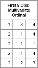
print first[label=“First 5 Obs: Multivariate Ordinal”];

Figure 9.4 A Few Simulated Observations

The X matrix is 1000 × 3 for this example. You can check the sample mean and sample variance, and compare them to the expected values that are shown in Figure 9.3:

mv = mean(X) // var(X); 
corr = corr(X); 
varNames = “X1”: “X3”;
print mv[r={“Mean” “Var”} c=varNames], corr;

Figure 9.5 Sample Mean and Correlation for Ordinal Data

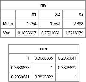
The sample means and variances are close to the population values. The sample correlations are close to the specified correlation matrix.

Exercise 9.2: Write the X matrix to a data set, and use PROC FREQ to compute the sample percentages of each category for the ordinal variables. Compare the sample percentages to the PMF for each variable.

Exercise 9.3: Use the TIME function to time how long it takes to generate a million observations for three correlated ordinal variables. The algorithm presented here is orders of magnitude faster than the algorithm in Kaiser, Träger, and Leisch (2011).

9.4 Reordering Multivariate Data: The Iman-Conover Method

The Iman-Conover method (Iman and Conover 1982) is a clever technique that combines p univariate distributions into a multivariate distribution for which the marginal distributions are exactly the same as the original univariate distributions. Furthermore, pairs of variables in the multivariate distribution have a rank correlation that is close to a specified target value. A rank correlation is a nonparametric measure of association that is computed by using the ranks of the data values rather than using the values themselves. The CORR procedure can compute the Spearman rank-order correlation.

The Iman-Conover method enables you to specify any data (simulated or real) for the marginal distributions. The only other input needed is the target rank correlation matrix.

Iman and Conover carefully describe each step of the construction and give an example for constructing six correlated variables. Their paper is very readable and so this book does not repeat their arguments. The main idea is as follows. Suppose M is a simulated N × p data matrix. Compute the ranks of the elements in each column of M. By definition, any matrix that has columns with the same ranks as M also has the same rank correlation as M. Therefore, given any N × p matrix Y, sort each column so that the column has the same ranks as the corresponding column in M. The rearranged version of Y has the specified rank correlation, but you have not changed the marginal distribution of the Y data because all you did was rearrange the columns.

The Iman-Conover article shows how to generate a matrix M that has (approximately) a given rank correlation. (This is the main contribution of the article.) There is nothing random in the Iman-Conover method. That is, given a rank correlation, the algorithm constructs the same matrix M every time. Therefore, the randomness in a simulation comes from simulating the marginal distributions of Y. The Iman-Conover algorithm simply rearranges the elements of columns of your data matrix.

The following SAS/IML program defines a function that reorders the elements in each column of a data matrix, Y, so that it has approximately the rank correlation given by the matrix C:

/* Use Iman-Conover method to generate MV data with known marginals
   and known rank correlation. */
proc iml;
start ImanConoverTransform(Y, C); 
    X = Y;
    N = nrow(X); 
    R = J(N, ncol(X));
    /* compute scores of each column */ 
    do i = 1 to ncol(X);
       h = quantile(“Normal”, rank(X[,i])/(N+1) );
       R[,i] = h;
    end;
    /* these matrices are transposes of those in Iman & Conover */ 
    Q = root(corr(R)); 
    P = root(C);
    S = solve(Q,P);       /* same as S = inv(Q) * P; */
    M = R*S;       /* M has rank correlation close to target C */


    /* reorder columns of X to have same ranks as M.
       In Iman-Conover (1982), the matrix is called R_B. */ 
    do i = 1 to ncol(M); 
       rank = rank(M[,i]);
       y = X[,i];
       call sort(y); 
       X[,i] = y[rank]; 
    end;
    return( X ); 
 finish;

To test the algorithm, simulate data vectors from various distributions and pack the vectors into columns of a matrix, A, as follows:

/* Step 1: Specify marginal distributions */ 
call randseed(1);
N = 100;
A = j(N,4); y = j(N,1);
distrib = {“Normal” “Lognormal” “Expo” “Uniform”}; 
do i = 1 to ncol(distrib);
   call randgen(y, distrib[i]); 
   A[,i] = y; 
end;

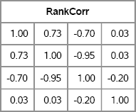
This example generates data from one normal distribution and three nonnormal distributions. To obtain a specified target rank correlation without changing the marginal distributions, call the Iman-Conover algorithm. Figure 9.6 shows that the rank correlation of X is close to the specified rank correlation matrix, C.

/* Step 2: specify target rank correlation */ 
C = { 1.00 0.75 -0.70 0, 
      0.75 1.00 -0.95 0, 
     -0.70 -0.95 1.00 -0.2, 
      0     0   -0.2   1.0};

X = ImanConoverTransform(A, C); 
RankCorr = corr(X, “Spearman”); 
print RankCorr[format=5.2];

Figure 9.6 Rank Correlation for Simulated Data with Specified Marginals

You can visualize the simulated data to show that the marginal distributions are normally, lognormally, exponentially, and uniformly distributed, respectively. Figure 9.7 shows that the marginal distributions appear to have the specified distributions, and the pairwise correlations also appear to be as specified.

/* write to SAS data set */
create MVData from X[c=(“x1”:“x4”)]; append from X; close MVData; 
quit;

proc corr data=MVData Pearson Spearman noprob plots=matrix(hist);
   var x1-x4; 
run;

Exercise 9.4: Use PROC UNIVARIATE to fit the lognormal and exponential distributions to the x2 and x3 variables, respectively.

Figure 9.7 Univariate and Bivariate Distributions of Simulated Data

9.5 Generating Data from Copulas

Each of the previous sections describes how to combine marginal distributions (binary, ordinal, or arbitrary) to obtain a joint distribution with a specified correlation. The word “copula” means to link or join, and that is exactly what a mathematical copula does: It creates a multivariate distribution by joining univariate marginal distributions.

Copulas are mathematically sophisticated, and the copula literature is not always easy to read. However, the good news is that you can use copulas to simulate data without needing to understand all the details of their construction. This section begins with a motivating example, and then discusses some of the theory behind copulas. Section 9.5.3 describes how to use the COPULA procedure in SAS/ETS software to simulate data.

9.5.1 A Motivating Example

Suppose that you want to simulate data from a bivariate distribution that has the following properties:

• The correlation between the variables is 0.6.
• The marginal distribution of the first variable is Gamma(4) with unit scale.
• The marginal distribution of the second variable is standard exponential.

How might you accomplish this? One approach would be to try to transform a set of bivariate normal variables. It is easy to simulate multivariate normal data with a desired correlation, so perhaps you can transform the normal variates to match the desired marginal distributions. There is no reason to think that the transformed variates will have the same correlation as the normal variates, but ignore that problem for now.

Start by simulating multivariate normal data, as shown in the following SAS/IML statements:

proc iml;
call randseed(12345); 
Sigma = {1.0 0.6, 
         0.6 1.0}; 
Z = RandNormal(1e4, {0,0}, Sigma);

The matrix Z contains 10,000 observations drawn from a bivariate normal distribution with correlation coefficient ρ = 0.6. (With 10,000 observations, the density of Z closely matches the density of the MVN distribution.) To transform the columns, you can use the following basic probability fact:

Fact 1: If F is the cumulative distribution function of a continuous random variable, X, then the random variable U = F(X) is distributed as U(0,1). The random variable U is called the grade of X.

This fact is very useful. It means that you can transform the normal variates into uniform variates by applying Φ, which is the cumulative distribution function for the univariate normal distribution. In SAS, the CDF function applies the cumulative distribution function, as follows:

U = cdf(“Normal”, Z);     /* columns of U are U(0,1) variates */

The columns of U are samples from a standard uniform distribution. However, they are not independent. They have correlation because they are a transformation of correlated variables.

Uniform variates are useful because they are easy to transform into any distribution: Just apply Fact 1 again. To make it easier to apply, rewrite Fact 1 in terms of the inverse CDF:

Fact 2: If U is a uniform random variable on [0, 1] and F is the cumulative distribution function of a continuous random variable, then the random variable X = F^–1(U) is distributed as F.

This formulation implies that you can obtain gamma variates from the first column of U by applying the inverse gamma CDF. Similarly, you can obtain exponential variates from the second column of U by applying the inverse exponential CDF. In SAS, the QUANTILE function applies the inverse CDF, as follows:

gamma = quantile(“Gamma”, U[,1], 4);   /* gamma ~ Gamma(alpha=4) */
expo = quantile(“Expo”, U[,2]);        /* expo ~ Exp(1) */
X = gamma || expo;

At this point, you have generated correlated bivariate observations. The first column of X contains gamma variates and the second column contains exponential variates. However, it is not clear whether the variates have the desired correlation of ρ = 06. The following statements compute the correlation coefficients for the original normal variates and for the transformed variates:

/* if Z~MVN(0,Sigma), corr(X) is often close to Sigma, 
   where X=(X1,X2,…,Xm) and X_i = F_i^{-1}(Phi(Z_i)) */ 
rhoZ = corr(Z)[1,2];           /* extract corr coefficient */
rhoX = corr(X)[1,2]; 
print rhoZ rhoX;

Figure 9.8 Sample Correlation Coefficients for Normal and Transformed Variates, ρ = 0.6

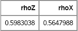
As expected, the sample correlation of the normal variates is very close to the target value of 0.6. The correlation of the transformed variates is not as close, and a two-sided 95% confidence interval for the correlation coefficient does not include 0.6 (see Exercise 9.5).

However, perhaps this approach can be modified. Suppose that you run a computer experiment to study the relationship between the correlation of the normal variates and the correlation of the transformed variates. Suppose that the experiment reveals that the sample correlation for the transformed variables is a monotone function of ρ. This implies that there is some value ρ* such that if normal variates are drawn from a bivariate normal distribution with correlation ρ*, then the transformed variables will have the desired target correlation of 0.6. The following statements carry out this experiment. The results are shown in Figure 9.9.

/* even though corr(X) ^= Sigma, you can often choose a target
   correlation, such as 0.6, and then choose Sigma so that corr(X) 
   has the target correlation. */ 
Z0=Z; U0=U; X0=X;     /* save original data */
Sigma = I(2);
rho = T( do(0.62, 0.68, 0.01) ); 
rhoTarget = j(nrow(rho), 1); 
do i = 1 to nrow(rho);
    Sigma[1,2]=rho[i]; Sigma[2,1]=Sigma[1,2];
    Z = RandNormal(1e4, {0,0}, Sigma);     /* Z ~ MVN(0,Sigma) */ 
    U = cdf(“Normal”, Z);                  /* U_i ~ U(0,1)     */ 
    gamma = quantile(“Gamma”, U[,1], 4);   /* X_1 ~ Gamma(4)   */ 
    expo = quantile(“Expo”, U[,2]);        /* X_2 ~ Expo(1)    */ 
    X = gamma||expo;
    rhoTarget[i] = corr(X)[1,2];           /* corr(X) = ?      */ 
end;
print rho rhoTarget[format=6.4];

Figure 9.9 Sample Correlation Coefficients for Normal and Transformed Variates, 0.6 ≤ ρ ≤ 0.7

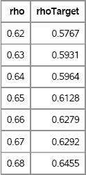
Given a target correlation ρ₀ = 0.6 for the transformed variables, Figure 9.9 shows that it is possible to choose a so-called intermediate correlation, ρ* ≈ 0.64, for the normal variates so that the desired correlation is achieved. The value of the intermediate correlation depends on the target value and on the specific forms of the marginal distributions.

Finding the intermediate value often requires finding the root of an equation that involves the CDF and inverse CDF. In fact, Step 2 in Section 9.2 is an example of using such an equation to generate correlated multivariate binary data.

This example generalizes to multivariate data. A copula is an abstraction of these ideas, but the example contains all of the main ideas of copulas. If you read the multivariate simulation literature, then you will see variations of this approach over and over again.

As many authors have remarked and as is shown in Section 9.4, if you use rank correlation (for example, Spearman's correlation), then the problem of finding an intermediate correlation vanishes. Because rank correlations are invariant under monotonic transformations of the data, the rank correlations of Z, U, and X are equal, as shown in Figure 9.10:

RankCorrZ = corr(Z0, “Spearman”)[1,2]; 
RankCorrU = corr(U0, “Spearman”)[1,2]; 
RankCorrX = corr(X0, “Spearman”)[1,2]; 
print RankCorrZ RankCorrU RankCorrX;

Figure 9.10 Rank Correlations, ρ = 0.6

Although the uniform variates seem to be an intermediate step, they are important because they can be used to visualize the joint dependence between the marginal distributions. In fact, it is instructive to visualize the dependencies between each of the three sets of variables: the normal variates (Z), the uniform variates (U), and the transformed variates (X). The following statements write these variables to a SAS data set for further analysis:

Q = Z||U||X;
labels = {Z1 Z2 U1 U2 X1 X2}; 
create CorrData from Q[c=labels]; 
append from Q; 
close CorrData;

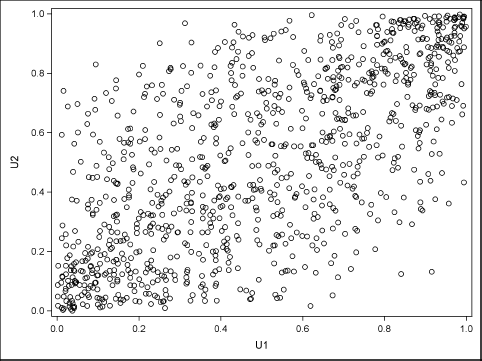
You can use PROC CORR or PROC SGPLOT to create a scatter plot of the correlated uniform variates. The following statement creates the scatter plot, which is shown in Figure 9.11. The plot shows the copula of the joint distribution:

proc sgplot data=CorrData(obs=1000);
   scatter x=U1 y=U2; 
run;

Figure 9.11 Plot of Uniform Variates Showing the Dependence Structure

Exercise 9.5: The FISHER option in the PROC CORR statement computes a confidence interval for the correlation and can test the hypothesis that it has a specified value. Verify that the 95% two-sided confidence interval for the correlation coefficient contains 0.6 and that the null hypothesis (ρ = 0.6) is not rejected. Repeat the analysis for the X1 and X2 variables.

Exercise 9.6: Create a scatter plot and histograms of the X1 and X2 variables in the CorrData data set.

9.5.2 The Copula Theory

The example in the previous section is an example of a “normal copula” (Nelsen 1999). Two gentle introductions to an otherwise formidable subject are Meucci (2011) and Channouf and L'Ecuyer (2009). In certain engineering fields, the normal copula is known as the NORTA method, where NORTA means “NORmal To Anything” (Cario and Nelson 1997). This exposition follows Channouf and L'Ecuyer (2009). Although this section is written for the relatively simple case of a normal copula and continuous marginals, many of the ideas also apply to general classes of copulas and to distributions with discrete marginals.

As described in the previous section, the goal is to simulate from a joint multivariate distribution with a specified correlation and a specified set of marginal distributions. Sklar's theorem (Schmidt 2007) says that every joint distribution can be written as a function (called the copula) of the marginal distributions. The word “copula” means to link or join, and that is exactly what a mathematical copula does: It joins the marginal distributions in such a way as to form a joint distribution with a given correlation structure.

For completeness, here is the formal definition. Let X = (X₁, X₂, … , X_m) be a random vector with marginal cumulative distribution functions F_X1, F_X2, … , F_Xm. Sklar's theorem says that the joint distribution function, F_X, can be written as a function of the marginal distributions:

F_X(x) = C(F_X1(x₁), … , F_Xm(x_m))

where x = (x₁, … , x_m) and C : [0,1]^m → [0,1] is a joint distribution function of the random variables U_i = F_xi(X_i).

Notice two points. First, if the X_i are independent, then the copula function is simply the product function C(u₁ , … , u_m) = ∏_iu_i, and the corresponding density function for the copula is the constant function, 1. Second, Figure 9.11 is a graph that helps to visualize the copula function. The copula function for the example is approximated by the empirical cumulative distribution that is shown in the scatter plot.

The beauty of the copula approach is that the copula separates the problem of modeling the marginals from the problem of fitting the correlations between the variables. These two steps can be carried out independently. The copula also makes it easy to simulate data from the model: Generate correlated uniform variates according to the copula (as in Figure 9.11), and then generate the random variates for each coordinate by applying the appropriate inverse distribution function: The generation of the random uniform variates depends on the choice of the copula, but for a normal copula you can use the technique in Section 9.5.1.

9.5.3 Fitting and Simulating Data from a Copula Model

In SAS software, you can use the MODEL procedure or the COPULA procedure in SAS/ETS software to fit a copula to data and to simulate from the copula (Erdman and Sinko 2008; Chvosta, Erdman, and Little 2011). This section uses the COPULA procedure to fit a normal copula model and to simulate data with similar characteristics. For more complicated examples, see the cited papers and the documentation for the COPULA procedure in the SAS/ETS User's Guide.

Rank (Spearman) correlations, rather than Pearson correlations, are used by PROC COPULA and by many who use copulas. In copula theory, there are three primary kinds of dependence structures (Schmidt 2007): Pearson correlation, rank correlation, and tail dependence. The classical Pearson correlation is a suitable measure of dependence only for the so-called “elliptical distributions,” which includes normal copulas, Student t copulas, and their mixtures. Outside of this class of distributions, Pearson correlations are unwieldy to work with because of the following shortcomings (Schmidt 2007, p. 14):

• Pearson correlations are not invariant under general monotonic transformation.
• As was shown for multivariate binary variables in Section 9.2, for specified marginal distributions there might be Pearson correlations that are unattainable.

In contrast, rank correlations do not suffer from these shortcomings.

The copula process proceeds in four steps:

1. Model the marginal distributions.
2. Choose a copula from among those supported by PROC COPULA. Fit the copula to the data to estimate the copula parameters. For this example, a normal copula is used, so the parameters are the six pairwise correlation coefficients that make up the upper-triangular correlation matrix of the data.
3. Simulate from the copula. For the normal copula, this consists of generating multivariate normal data with the given rank correlations. These simulated data are transformed to uniformity by applying the normal CDF to each component.
4. Transform the uniform marginals into the marginal distributions by applying the inverse CDF for each component.

For this example, use the MVData data set that is described in Section 9.4. Assume that Step 1 is complete and that the following models describe each marginal distribution:

• The X1 variable is modeled by a standard normal distribution.
• The X2 variable is modeled by a standard lognormal distribution.
• The X3 variable is modeled by a standard exponential distribution.
• The X4 variable is modeled by a uniform distribution on [0,1].

Steps 2 and 3 are accomplished by using the COPULA procedure. Step 2 is accomplished with the FIT statement and Step 3 is accomplished with the SIMULATE statement, as shown in the following call to PROC COPULA:

/* Step 2: fit normal copula
   Step 3: simulate data, transformed to uniformity */ 
proc copula data=MVData; 
   var x1-x4; 
   fit normal;
   simulate / seed=1234 ndraws=100
               marginals=empirical outuniform=UnifData;
run;

The UnifData data set contains the transformed simulated data. You can apply the final transformation by using the QUANTILE function for each component to recover the modeled form of the marginals:

/* Step 4: use inverse CDF to invert uniform marginals */ 
data Sim; 
set UnifData;
lognormal = quantile(“Normal”, x1); 
lognormal = quantile(“LogNormal”, x2); 
expo = quantile(“Exponential”, x3); 
uniform = x4; 
run;

You can use PROC CORR to compute the rank correlations of the original and simulated data. You can also create a matrix of scatter plots that display the pairwise dependencies between the original and the simulated data.

/* Compare original distribution of data to simulated data */ 
proc corr data=MVData Spearman noprob plots=matrix(hist); 
   title “Original Data”; 
   var x1-x4; 
run;

proc corr data=Sim Spearman noprob plots=matrix(hist); 
   title “Simulated Data”; 
   var normal lognormal expo uniform; 
run;

Figure 9.12 Original Data

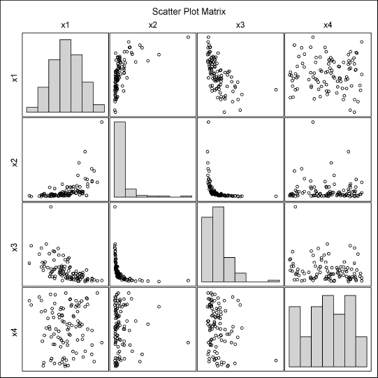
Figure 9.13 Data Simulated from a Copula

The Spearman rank correlation matrices are not shown, but the Spearman correlations of the variables in the Sim data set are close to those in the MVData data set. The scatter plot matrices are shown in Figure 9.12 and Figure 9.13. They look very similar. Unfortunately, PROC COPULA does not provide any goodness-of-fit statistics or an indication of whether the copula model is a good model for the data.

You can simulate many samples from the COPULA function by using a single call. For example, to simulate 100 samples of size 20, use the %SYSEVALF macro to generate the product of these numbers:

%let N = 20;
%let NumSamples=100;
proc copula data=MVData;

     …
     simulate / ndraws=%sysevalf(&N*&NumSamples) outuniform=UnifData;
     …

You can then use a separate DATA step to assign values for the usual SampleID variable, as follows:

data UnifData; 
set UnifData;
SampleID = 1 + floor((_N_-1) / &N); 
run;

Exercise 9.7: Use the FISHER option in the PROC CORR statement to compute 95% confidence intervals for the Spearman correlation of the variables in the Sim data set. Show that these confidence intervals contain the parameter values in Section 9.4 that generated the data.

9.6 References

Cario, M. C. and Nelson, B. L. (1997), Modeling and Generating Random Vectors with Arbitrary Marginal Distributions and Correlation Matrix, Technical report, Northwestern University.

Channouf, N. and L'Ecuyer, P. (2009), “Fitting a Normal Copula for a Multivariate Distribution with Both Discrete and Continuous Marginals,” in M. D. Rossetti, R. R. Hill, B. Johansson, A. Dunkin, and R. G. Ingalls, eds., Proceedings of the 2009 Winter Simulation Conference, 352-358, Piscataway, NJ: Institute of Electrical and Electronics Engineers.

Chvosta, J., Erdman, D., and Little, M. (2011), “Modeling Financial Risk Factor Correlation with the COPULA Procedure,” in Proceedings of the SAS Global Forum 2011 Conference, Cary, NC: SAS Institute Inc.
URL http://support.sas.com/resources/papers/proceedings11/340-2011.pdf

Demirtas, H. (2006), “A Method for Multivariate Ordinal Data Generation Given Marginal Distributions and Correlations,” Journal of Statistical Computation and Simulation, 76, 1017-1025.

Emrich, L. J. and Piedmonte, M. R. (1991), “A Method for Generating High-Dimensional Multivariate Binary Variables,” American Statistician, 45, 302-304.

Erdman, D. and Sinko, A. (2008), “Using Copulas to Model Dependency Structures in Econometrics,” in Proceedings of the SAS Global Forum 2008 Conference, Cary, NC: SAS Institute Inc.
URL http://support.sas.com/resources/papers/sgf2008/copulas.pdf

Iman, R. L. and Conover, W. J. (1982), “A Distribution-Free Approach to Inducing Rank Correlation among Input Variables,” Communications in Statistics—Simulation and Computation, 11, 311-334.

Kaiser, S., Träger, D., and Leisch, F. (2011), Generating Correlated Ordinal Random Values, Technical report, University of Munich, Department of Statistics.
URL http://epub.ub.uni-muenchen.de/12157/

Meucci, A. (2011), “A Short, Comprehensive, Practical Guide to Copulas,” Social Science Research Network Working Paper Series.
URL http://ssrn.com/abstract=1847864

Nelsen, R. B. (1999), An Introduction to Copulas, New York: Springer-Verlag.

Oman, S. D. (2009), “Easily Simulated Multivariate Binary Distributions with Given Positive and Negative Correlations,” Computational Statistics and Data Analysis, 53, 999-1005.

Schabenberger, O. and Gotway, C. A. (2005), Statistical Methods for Spatial Data Analysis, Boca Raton, FL: Chapman & Hall/CRC.

Schmidt, T. (2007), “Coping with Copulas,” in J. Rank, ed., Copulas: From Theory to Application in Finance, 3-34, London: Risk Books.