CHAPTER 13
Volume Controls
Volume Controls
A volume control is the most essential knob on a preamplifier –in fact, the unhappily named “passive preamplifiers” usually consist of nothing else but a volume control and an input selector switch. Volume controls in one guise or another are also freely distributed on the control surfaces of mixing consoles, examples being the auxiliary sends and the faders.
A volume control for a hi-fi preamplifier needs to cover at least a 50 dB range, with a reasonable approach to a logarithmic (i.e. linear-in dB) law, and have a channel balance better than ±1 dB over this range if noticeable stereo image shift is to be avoided when the volume is altered.
The simplest volume control is a potentiometer. These components, which are invariably called “pots” in practice, come with various control laws, such as linear, logarithmic, anti-logarithmic, and so on. The control law is still sometimes called the “taper” which is a historical reference to when the resistance element was actually physically tapered, so the rate of change of resistance from track-end to wiper could be different at different angular settings. Pots are no longer made this way, but the term has stuck around. An “audio-taper” pot usually refers to a logarithmic type intended as a volume control.
All simple volume controls have the highest output impedance at the wiper at the –6 dB setting. For a linear pot, this is when the control is rotated halfway towards the maximum, at the 12 o’clock position. For a log pot, it will be at a higher setting, around 3 o’clock. The maximum impedance is significant because it usually sets the worst-case noise performance of the following amplification stage. The resistance value of a volume control should be as low as possible, given the loading/distortion characteristics of the stage driving it. This is sometimes called “low-impedance design”. Lower resistances mean:
- Less Johnson noise from the pot track resistance
- Less noise from the current-noise component of the following stage
- Less likelihood of capacitive crosstalk from neighbouring circuitry
- Less likelihood of hum and noise pickup.
Volume Control Laws
What constitutes the optimal volume control law? This is not easy to define. One obvious answer is a strictly logarithmic or linear-in-dB law, but this is in fact somewhat less than ideal, as an excessive amount of the pot rotation is used for very high and very low volume settings that are rarely used. It is therefore desirable to have a law that is flatter in its central section but falls off with increasing rapidity towards the low-volume end –see the fader law later in this chapter. Sometimes the law steepens at the high-volume end as well, but this is somewhat less common.
A linear pot is a simple thing –the output is proportional to the angular control setting, and this is usually pretty accurate, depending on the integrity of the mechanical construction. Since the track is uniform resistance, its actual resistance makes no difference to the proportionality of the output unless it is significantly loaded by an external resistance. Unfortunately, a linear volume control law is quite unsatisfactory. The volume is only reduced from maximum by 6 dB at the halfway rotation point, but the steepness of the slope accelerates as it is turned further down. This can be seen as Trace 1 in Figure 13.3. Linear pots are usually given the code letter “B”. See Table 13.1 for more code letters.
Log pots are not, and do not attempt to be, precision attenuators with a fixed number of dB attenuation for each 10 degrees of shaft rotation. The track is not uniform but is made up of two or three linear slopes that roughly approximate a logarithmic law, produced by superimposing two or three sections of track made with different resistivity material. If two slopes are used, the overlap is towards the bottom end of the control setting, typically at 20% of full rotation; see Figure 13.1. The two materials of different resistivity have to match for the desired law to be obtained, and close matching is difficult to achieve, so log controls are rather less satisfactory in terms of accuracy; much more on that later. Looking at the log pot trace in Figure 13.1, we can see that the volume at half-rotation is now 20%, or 14 dB down, which is not really a great improvement on the 6 dB down we get with a linear pot. Log pots are usually given the code letter “A”.
Anti-logarithmic pots are the same only constructed backwards, so that the slope change is at the top end of the control setting; these are typically used as gain controls for amplifying stages rather than as volume controls. These pots are usually given the code letter “C”.
There is a more extreme version of the anti-logarithmic law in which the slope change occurs at 10% of rotation instead of 20%. These are useful where you want to control the gain of an amplifying stage over a wide range and still have something like a linear-in-dB control law. Typically they are used to set the gain of microphone input amplifiers, which can have a gain range of 50 dB or more. These pots are given the code “RD”, which stands for Reverse-D-law; I don’t think I have ever come across a non-reverse D-law. Some typical laws are shown in Figure 13.1.
| ALPS Code letter | Pot characteristic |
|---|---|
| A | Logarithmic |
| B | Linear |
| C | Anti–logarithmic |
| RD | Reverse–log |
Please note that the code letters are not adhered to quite as consistently across the world as one might hope. The codes given in Table 13.1 are those used by ALPS, one of the major pot makers, but other people use quite different allocations; for example Radiohm, another major manufacturer, calls linear pots A and log pots B, but they agree that anti-log pots should be called C. Radiohm has several other laws called F, T, S, and X; for example, S is a symmetrical law apparently intended for use in balance controls. It clearly pays to check very carefully what system the manufacturer uses when you’re ordering parts.
The closeness of approach to an ideal logarithmic law is not really the most important characteristic of a volume control; spreading out the most-used middle region is more useful. Of greater importance is the matching between the two halves of a stereo volume control. It is common for the channel balance of log pots to deteriorate quite markedly at low volume settings, causing the stereo image to shift as the volume is altered. You may take it from me that customers really do complain about this, and so a good deal of ingenuity has been applied in attempts to extract good performance from indifferent components.
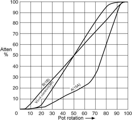
Figure 13.1 The control laws of typical linear and log pots.
An important point in the design of volume controls is that their offness – the amount of signal that gets through when the control is at its minimum – is not very critical. This is in glaring contrast to a level control such as an auxiliary send on a mixer channel (see Chapter 22), where the maximum possible offness is very important indeed. A standard log pot will usually have an offness in the order of -90 dB with respect to fully up, and this is quite enough to render even a powerful hi-fi system effectively silent.
Loaded Linear Pots
Since ordinary log pots are not very accurate, many other ways of getting a log law have been tried. Trace 1 in Figure 13.3 (for a linear pot with no loading) makes it clear that the use of an unmodified linear law for volume control really is not viable; the attenuation is all cramped up at the bottom end. A good approximation to a logarithmic law can be made by loading the wiper of a linear pot with a fixed resistor R1 to ground, as shown in Figure 13.2.

Figure 13.2 Resistive loading of a linear pot to approximate a logarithmic law.
Adding a loading resistor much improves the law, but the drawback is that this technique really only works for a limited range of attenuation –in fact, it only works well if you are looking for a control that varies from around 0 to -20 dB. It is therefore suitable for power amp level controls and aux master gain controls (see Chapter 22 for details of the latter) but is unlikely to be useful for a preamplifier gain control, which needs a much wider logarithmic range. Figure 13.3 shows how the law varies as the value of the loading resistor is changed, and it is pretty clear that whatever its value, the slope of the control law around the middle range is only suitable for emulating the ideal log law labelled “20”. The value of the loading resistor for each trace number is given in Table 13.2.
| Trace number | Loading resistor R1 value |
|---|---|
| 1 | None |
| 2 | 4k7 |
| 3 | 2k2 |
| 4 | 1 kΩ |

Figure 13.3 Resistive loading of a linear pot: the control laws plotted.
Figure 13.3 shows that with the optimal loading value (Trace 2) the error in emulating a 0 to -20 dB log range is very small, lying within ±0.5 dB over the range 0 to -16 dB; below this, the error grows rapidly. This error for Trace 2 only is shown in Figure 13.4.

Figure 13.4 Loading of a linear pot: the deviation from an ideal 20 dB log law of Trace 2 in Figure 13.3.
Obtaining an accurate law naturally relies on having the right ratio between the pot track resistance and the loading resistor. The resistance of pot tracks is not controlled as closely as fixed resistors, their tolerance usually being specified as ±20%, so this presents a significant balance-shift problem. The only solution would seem to be making the loading resistor trimmable, and this approach has been used in a master volume control by at least one console manufacturer.
Figure 13.5 shows the effect on the control law of a ±20% pot track tolerance, with a loading resistor of 4k7 that is assumed to be accurate (Trace 2 in Figure 13.3). With the pot track 20% low in value, the loading resistor has less effect, and we get the dotted line above the solid (nominal) line. If it is 20% high, the loading resistor has more effect, giving the lower dotted line. The error around the middle of control rotation is about ±0.7 dB, which is enough to give perceptible balance errors in a stereo volume control. If you are unlucky enough to have the two tracks 20% out in opposite directions, the error will be 1.4 dB.
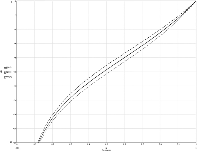
Figure 13.5 The effect of a ±20% pot track tolerance, with 4k7 resistive loading.
Another snag to this approach is that when the control is fully up, the loading resistor is placed directly across the input to the volume control, reducing its impedance drastically and possibly causing unhappy loading effects on the stage upstream. However, the main problem is that you are stuck with a 0 to -20 dB range, inadequate for a volume control on a preamplifier.
The following stage must have a high enough impedance to not significantly affect the volume control law; this obviously also applies to plain logarithmic pots and to all the passive controls described here.
Dual-Action Volume Controls
In the previous section on loaded linear pots, we have seen that the control law is only acceptably logarithmic over a limited range –too limited for effective use as a volume control in a preamplifier or as a fader or send control in a mixer. One way to fix this is the cascading of pots, so that their attenuation laws sum in dB. This approach does of course require the use of a four-gang pot for stereo, which may be objectionable because of increased cost, possible problems in sourcing, and a worsened volume-control feel. Nonetheless, the technique can be useful, so we will give it a quick look.

Figure 13.6 Dual-action volume controls: a) shows two linear pots cascaded, and b) is a linear pot cascaded with a loaded-linear pot.
It is assumed there is no interaction between the two pots, so the second pot does not directly load the wiper of the first. This implies a buffer stage between them, as shown in Figure 13.6. There is no need for this to be a unity-gain stage, and in fact, several stages can be interposed between the two pots. This gives what is usually called a distributed gain control, which can be configured to give a better noise/headroom compromise than a single volume control.

Figure 13.7 shows a linear law (Trace 1) and the square-law (Trace 2) made by cascading two linear pots. 20 dB and 30 dB ideal log lines are shown for comparison, and it is pretty clear that while the square law is much more usable than the linear law, it is still a long way from perfect. It does, however, have the useful property that, assuming the wiper is very lightly loaded by the next stage, the gain is dependant only upon control rotation and not the ratio between fixed 1% resistors and a ±20% pot track resistance. Figure 13.8 shows the deviation of the square-law from the 30 dB line; the error peaks at just over + 3 dB before it plunges negative.
A much better attempt at a log law can be made by cascading an unloaded linear pot with a loaded linear pot; the resulting law is shown in Figure 13.9. Trace 1 is the law of the linear pot alone, and Trace 2 is the law of a loaded linear 10 kΩ pot with a 2.0 kΩ loading resistor R1 from wiper to ground, alone. The combination of the two is Trace 3, and it can be seen that this gives a very good fit to a 40 dB ideal log line and good control over a range of at least 35 dB.
Figure 13.10 shows the deviation of the combined law from the 40 dB line; the law error now peaks at just over ±1 dB. Unfortunately, adding the loading resistor means that once more, the gain is dependent on the ratio between a fixed resistor and the pot track resistance.

Figure 13.8 Dual-action volume control: the deviation of the square law from the ideal 30 dB log line.

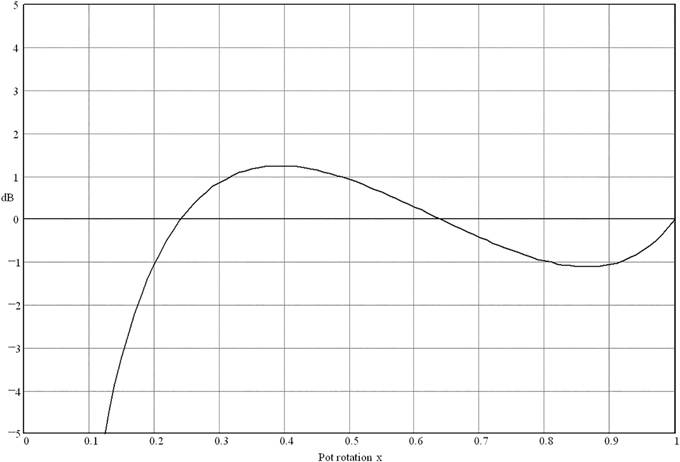
Figure 13.10 Dual-action volume control with improved law: deviation of the control law from the ideal 40 dB log line. Much better than Figure 13.8.
Passive volume controls of various types can of course also be cascaded with an active volume control stage, and this can be a good way to obtain a desired control law. This is dealt with later in this chapter.
Tapped Volume Controls
The control law of a linear pot can be radically altered if it has a centre tap (see Chapter 22 for the use of tapped pots for LCR panning). This can be connected to a potential divider that has a low impedance compared with the pot track resistance and the attenuation at the tap point altered independently of other parameters. Figure 13.11 shows both unloaded and loaded versions of the arrangement.
The unloaded version shown in Figure 13.11a is arranged so that the attenuation at the tap is close to -20 dB. This gives the law shown in Figure 13.12; it approximates to a 33 dB log line, but there is an abrupt change of slope as the pot wiper crosses the tapping point.
Note that the track resistance has to be a good deal higher than that of the fixed resistors so that they control the level at the tap. This means that with the values shown, the source impedance at the wiper can be as high as 12.5 kΩ when it is halfway between the tap and one end, and this may degrade the noise performance, particularly if the following stage has significant current noise. A normal 10 kΩ pot, of whatever law, has a maximum output impedance of only 2.5 kΩ. To match this figure, the values shown would have to be scaled down by a factor of 5, so that R1 = 2k, R2 = 200 Ω, and the track resistance is a more normal 10 kΩ. This scaling is quite practical, the load on the previous stage now being 1.62 kΩ.

Figure 13.11 Tapped volume control: a) unloaded; b) loaded; c) with active control of tap voltage.

Figure 13.12 The law of an unloaded tapped volume control with -20 dB at the tap.
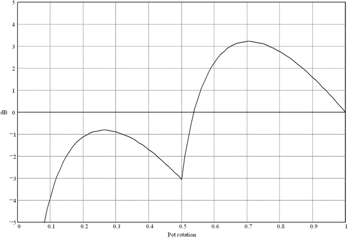
Figure 13.13 The deviation of the unloaded tapped volume control law from an ideal 33 dB log line.
The error is shown in Figure 13.13. This version of a tapped linear volume control covers a range of about 30 dB and almost keeps the errors within ±3 dB; but that abrupt change of slope at the tap point is somewhat less than ideal.
A much better approach to a log law is possible if a loading resistor is added to the wiper, as with the loaded linear pot already examined. See Figure 13.11b for the circuit arrangement and Figure 13.14 for the control law. If the resistors are correctly chosen, using the ratios given in Figure 13.11b, the law can be arranged to have no change of slope at the tapping, and the deviation from a 40 dB ideal line will be less than 1 dB over the range from 0 to -38 dB. The exact values of the resistors are given rather than the nearest preferred values. It is clear that this is a very effective way of giving an accurate law over a wide range, and it is widely used in making high-quality slide faders using multiple taps and a conductive plastic track. Note that the accuracy still depends on good control of the track resistance value compared with the fixed resistors.
If the value of the resistors connected to the tap is such that the loading effect on the previous stage becomes excessive, one possible solution is shown in Figure 13.11c, where the R1 and R2 are kept reasonably high in value, and a unity-gain opamp buffer now holds the tap point in a vise-like grip due to its low output impedance. The disadvantage is that the noise of the opamp, and of R1 in parallel with R2, is fed directly through at full level when the wiper is near the tap. Often this will be at a lower level than the noise from the rest of the circuitry, but it is a point to watch. Note that because of the low-impedance drive from the opamp, the values of the fixed resistors will need to be altered from those of Figure 13.11b to get the best control law.
If the best possible noise performance is required, then it is better to increase the drive capability of the previous stage and keep the resistors connected to the tap low in value; if this is done by paralleling opamps, then the noise performance will be improved rather than degraded.
Slide Faders
So far as the design of the adjacent circuitry is concerned, a fader can normally be regarded as simply a slide-operated logarithmic potentiometer. Inexpensive faders are usually made using the same two-slope carbon-film construction as are rotary log volume controls, but the more expensive and sophisticated types use a conductive-plastic track with multiple taps connected to a resistor ladder, as described in the previous section. This allows much better control over the fader law.
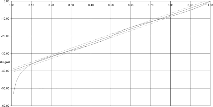
High-quality faders typically have a conductive-plastic track, contacted by multiple gold-plate metal fingers to reduce noise during movement. A typical law for a 104 mm travel fader is shown in Figure 13.15. Note that a fader does not attempt to implement a linear-in-dB log scale; the attenuation is spread out over the top part of the travel and much compressed at the bottom. This puts the greatest ease of control in the range of most frequent use; there is very little point in giving a fader precise control over signals at -60 dB.

Figure 13.16a shows the straightforward construction used in smaller and less expensive mixers. There is some end resistance Ref at the bottom of the resistive track which compromises the offness, and it is further compromised by the voltage-drop down the resistance Rg of the ground wire that connects the fader to the channel PCB. To fix this, a so-called infinity-off feature is incorporated into the more sophisticated faders.
Figure 13.16b shows an infinity-off fader. When the slider is pulled down to the bottom of its travel, it leaves the resistive track and lands on an end-section with a separate connection back to the channel module ground. No signal passes down this ground wire, and so there is no voltage-drop along its length. This arrangement gives extremely good maximum attenuation, orders of magnitude better than the simple fader, though of course “infinity” is always a tricky thing to claim.
Faders are sometimes fitted with fader-start switches; these are microswitches which are actuated when the slider moves from the “off” position. Traditionally, these started tape cartridge machines; now they may be used to trigger digital replay.

Active Volume Controls
Active volume controls have many advantages. As explained in the section on preamplifier architectures. the use of an active volume control removes the dilemma concerning how much gain to put in front of the volume control and how much to put after it. An active gain control must fulfil the following requirements:
- The gain must be smoothly variable from a maximum, usually well above unity, down to effectively zero, which in the case of a volume control means at least -70 dB. This at once rules out series-feedback amplifier configurations, as these cannot give a gain of less than 1 unless combined with a following passive control. Since the use of shunt feedback implies a phase inversion, this can cause problems with the preservation of absolute polarity.
- The control law relating shaft rotation and gain should be a reasonable approximation to a logarithmic law. It does not need to be strictly linear-in-decibels over its whole range; this would give too much space to the high-attenuation end, say around -60 dB, and it is better to spread out the middle range of -20 to -50 dB, where the control will normally be used. These figures are naturally approximate, as they depend on the gain of the power amplifier, speaker sensitivity, and so on. A major benefit of active gain controls is that they give much more flexible opportunities for modifying the law of a linear pot than does the simple addition of a loading resistor, which was examined and found somewhat wanting earlier in this chapter.
- The opportunity to improve channel balance over the mediocre performance given by the average log pot should be firmly grasped. Most active gain controls use linear pots and arrange the circuitry so that these give a quasi-logarithmic law. This approach can be configured to remove channel imbalances due to the uncertainties of dual-slope log pots.
- The noise gain of each amplifier involved should be as low as possible.
- As for passive volume controls, the circuit resistance values should be as low as practicable to minimise Johnson noise and capacitive crosstalk.

Figure 13.17 shows a collection of possible active volume configurations, together with their gain equations. Each amplifier block represents an inverting stage with a large gain -A, i.e. enough to give plenty of negative feedback at all gain settings. It can be regarded as an opamp with its non-inverting input grounded. Figure 13.17a simply uses the series resistance of a log pot to set the gain. While you get the noise/headroom benefits of an active volume control, the retention of a log pot with its two slopes and resulting extra tolerances means that the channel balance is no better than that of an ordinary passive volume control using a log pot. It may in fact be worse, for the passive volume control is truly a potentiometer, and if it is lightly loaded, differences in track resistance due to process variations should at least partially cancel, and one can at least rely on the gain being exactly 0 dB at full volume. Here, however, the pot is actually acting as a variable resistance, so variations in its track resistance compared with the fixed R1 will cause imbalance; the left and right gain will not even be the same with the control fully up. Given that pot track resistances are usually subject to a ±20% tolerance, it would be possible for the left and right channel gains to be 4 dB different at full volume. This configuration is not recommended.
Figure 13.17b improves on Figure 13.17a by using a linear pot and attempting to make it quasi-logarithmic by putting the pot into both the input and feedback arms around the amplifier. It is assumed that a maximum gain of 20 dB is required; it is unlikely that a preamplifier design will require more than that. The result is the law shown in Figure 13.18, which can be seen to approximate fairly closely to a linear-in decibels line with a range of -24 to +20 = 44 dB. This is a result of the essentially square-law operation of the circuit, in which the numerator of the gain equation increases as the denominator decreases. This is in contrast to the loaded linear pot case described earlier, which approximates to a 20 dB line.

Figure 13.18 The control law of the active volume control in Figure 13.17b.
The deviation of the control law from the 44 dB line is plotted in Figure 13.19, where it can be seen that between control rotations of 0.1 and 1 and a gain range of almost 40 dB, the maximum error is ±2.5 dB. This sort of deviation from an ideal law is not very noticeable in practice. A more serious issue is the way the gain heads rapidly south at rotations less than 0.1, with the result that volume drops rapidly towards the bottom of the travel, making it more difficult to set low volumes to be where you want them. Variations in track resistance tend to cancel out for middle volume settings, but at full volume, the gain is once more proportional to the track resistance and therefore subject to large tolerances.

Figure 13.19 The deviation of the control law in Figure 13.18 from an ideal 44 dB logarithmic line.
The configuration in Figure 13.17c also puts the pot into an input arm and a feedback arm, but in this case in separate amplifiers: the feedback arm of A1 and the input arm of A2. It requires two amplifier stages, but as a result, the output signal is in the correct phase. When configured with R = 10 kΩ, R1 = 10 kΩ, R3 = 1 kΩ, and R4 =10 kΩ, it gives exactly the same law as Figure 13.17b, with the same maximum error of ±2.5 dB. It therefore may be seen as pointless extra complication, but in fact the extra resistors involved give a greater degree of design freedom.
In some cases, a linear-in decibels line with a range of 44 dB, which is given by the active gain stages already looked at, is considered too rapid; less steep laws can be obtained from a modified version of Figure 13.17c, by adding another resistor R2 to give the arrangement in Figure 13.17d. This configuration was used in the famous Cambridge Audio P50 integrated amplifier, introduced in 1970. When R2 is very high, the law approximates to that of Figure 13.17c, see Trace 1 in Figure 13.20. With R2 reduced to 4 kΩ, the law is modified to Trace 2 in Figure 13.20; the law is shifted up, but in fact the slope is not much altered and is not a good approximation to the ideal 30 dB log line, labelled “30”. When R2 is reduced to 1 kΩ, the law is as Trace 3 in Figure 13.20 and is a reasonable fit to the ideal 20 dB log line, labelled “20”. Unfortunately, varying R2 can do nothing to help the way that all the laws fall off a cliff below a control rotation of 0.1, and in addition, the problem remains that the gain is determined by the ratio between fixed resistors, for which a tolerance of 1% is normal, and the pot track resistance, with its ±20% tolerance. For this reason, none of the active gain controls considered so far are going to help with channel balance problems.

Figure 13.20 The control law of the active volume control in Figure 13.17d.
The Baxandall Active Volume Control
The active volume control configuration in Figure 13.17e is due to Peter Baxandall. Like so many of the innovations conceived by that great man, it authoritatively solves the problem it addresses. [1] Figure 13.21 shows the law obtained with a maximum gain of +20 dB; the best-fit ideal log line is now 43 dB. There is still a rapid fall-off at low control settings.
You will note that there are no resistor or track resistance values in the gain equation in Figure 13.17e; the gain is only a function of the pot rotation and the maximum gain set up by R1, R2. As a result, quite ordinary dual linear pots can give very good channel matching. When I tried a number of RadioOhm 20 mm diameter linear pots, the balance was almost always within 0.3 dB over a 46 dB gain range, with occasional excursions to an error of 0.6 dB.
However, the one problem that the Baxandall configuration cannot solve is channel imbalance due to mechanical deviation between the wiper positions. I have only once found that the Baxandall configuration did not greatly improve channel balance; in that case, the linear pots I tried, which came from the same Chinese source as the log pots that were provoking customer irritation, had such poor mechanical alignment that the balance improvement obtained was small and not worth the extra circuitry. Be aware that there are some dual pots out there that have appreciable backlash between the two sections, and clearly the Baxandall approach cannot help with that.
Note that all the active gain configurations require a low-impedance drive if they are to give the designed gain range; don’t try feeding them from, say, the wiper of a balance control pot. The Baxandall configuration inherently gives a phase inversion that can be highly inconvenient if you are concerned to preserve absolute phase, but this can be undone by an inverting tone-control stage. Such as the Baxandall type…
An important point is that while at a first glance the Baxandall configuration looks like a conventional shunt feedback control, its action is modified by the limited gain set by R1 and R2. This means that the input impedance of the stage falls as the volume setting is increased but does not drop to zero. With the values shown in Figure 13.23, input impedance falls steadily from a maximum of 10 kΩ at zero gain, to a minimum of 1.27 kΩ at maximum gain. If the preceding stage is based on a 5532, it will have no trouble driving this. Another consequence of the gain of the A2 stage is that the signals handled by the buffer A1 are never very large. This means that R1, and consequently R2, can be kept low in value to reduce noise without placing an excessive load on the buffer.
All the active volume controls examined here, including the otherwise superior Baxandall configuration, give a gain law that falls very rapidly in the bottom tenth of control rotation. It is not easy to see that there is any cure for this.
The Baxandall Volume Control Law
While the Baxandall configuration has several advantages, it is not perfect. One disadvantage is that the gain/rotation law is determined solely by the maximum gain, and it is not possible to bend it about by adding resistors without losing the freedom from pot-value dependence.

Figure 13.21 The control law of the +20 dB Baxandall active volume control in Figure 13.17e.
Figure 13.22 shows the control laws for different maximum gains. Pot rotation is described here as Marks from Mk 0 to Mk 10 for full rotation. No provision is made for rock bands seeking controls going up to Mk 11. [2] Changing the maximum gain has a much smaller effect on the gain at the middle setting (Mk 5).
Very often, a maximum gain of +10 dB is required in preamplifier design, giving us -4 dB with the volume control central. In this case the control law is rather flat, with only 14 dB change of gain in the top half of control rotation. The +10 dB law approximates closely to a linear-in-decibels line with a range of -18 to +10 = 28 dB. This has a shallower slope than the 43 dB log line shown in Figure 13.21 and is not ideal for a volume control law. Things can be much improved by combining it with a linear law; more on this later.
A Practical Baxandall Active Volume Stage
I have designed several preamplifiers using a Baxandall active volume control. [3], [4], [5], [6] The practical circuitry I employed for [4] is shown in Figure 13.23; this includes DC-blocking arrangements to deal with the significant bias currents of the 5532 opamp. The maximum gain is set to +17 dB by the ratio of R1, R2 to amplify a 150 mV line input to 1 V with a small safety margin.

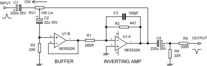
Figure 13.23 A practical Baxandall active volume control with DC blocking, as used in the Precision Preamplifier ’96.
| Setting | Noise out |
|---|---|
| Zero gain | –114.5 dBu |
| Unity gain | –107.4 dBu |
| Full volume | –90.2 dBu |
This active volume-control stage gives the usual advantages of lower noise at gain settings below maximum and excellent channel balance that depends solely on the mechanical alignment of the dual linear pot; all mismatches of its electrical characteristics are cancelled out. Note that in both the preamplifier designs referenced here, all the pots were identical at 10 kΩ linear, apart from the question of centre-detents, which are desirable only on the balance, and treble and bass boost/cut controls.
The values given here are as used in the Precision Preamplifier ’96. [4] Compared with [3], noise has been reduced slightly by an impedance reduction on the gain-definition network R1, R2. The limit on this is the ability of buffer U1:B to drive R1, which has a virtual earth at its other end. C3 ensures HF stability if there are excess phase shifts due to stray capacitance. C1 prevents any DC voltages from circuitry upstream from reaching the volume-control stage. The input bias current of U1:B will produce a small voltage drop across R3, and C2 prevents this from reaching the control pot. Since two terminals of the pot are DC blocked, it is now permissible to connect the third terminal directly to the output of U1:A, as no current can flow through the control. The offset voltage at the output of U1:B will be amplified by U1:A but should still be much too small to have any significant effect on available voltage swing, and it is prevented from leaving this stage by DC-blocking capacitor C4. R4 is a drain resistor to prevent voltage building up on the output due to leakage through C4, and R5 ensures stability by isolating the stage from load capacitance downstream, such as might be caused by the use of screened cable. Note that R4 is connected before R5 to prevent any loss of gain. The loss is of course very small in one stage, but it can build up irritatingly in a large system if this precaution is not observed. Table 13.3 gives the noise performance.
The figure at full volume may look a bit mediocre but results from the use of +17 dB of gain; at normal volume settings the noise output is well below -100 dBu.
Low-Noise Baxandall Active Volume Stages
One of the themes of this book is the use of multiple opamps to reduce noise, exploiting the fact that noise from uncorrelated sources partially cancels. The Baxandall volume stage lends itself very well to this technique, which is demonstrated in Figure 13.24. The first version at a) improves on the basic design in Figure 13.23 by using two inverting amplifiers instead of one and reducing the value of the pot from 10 kΩ to 5 kΩ. Bear in mind that the latter change reduces the input impedance proportionally, and it can fall to low values (1.2 kΩ in this case) with the volume control at maximum. The outputs of the two inverting amplifiers are averaged by the 10 Ω resistors R4 and R7, and the noise from them partially cancels. The noise from the unity-gain buffer U1:A is not reduced because it is reproduced identically by the two inverting amplifiers. C1 and R1 prevent the input bias current of the buffer from flowing through the pot wiper and causing rustling noises. This volume control stage was used in the variable-frequency-tone-control preamplifier published in Jan Didden’s Linear Audio, Volume 5. [5]

Note that in Figure 13.24a there is a spare opamp section floating in space. If this is not required elsewhere in the signal path, pressing it into use as another inverting amplifier will usually give more noise reduction than doubling up the buffer.
Figure 13.24b shows a more sophisticated design for still lower noise, using four inverting amplifiers and four separate buffers. There is nothing to be gained by averaging the buffer outputs before applying the signal to the inverting amplifiers, as the partial cancellation of buffer noise is carried out later by the 10 Ω resistors R103, etc., just as for the inverting amplifier noise. Four inverting amplifiers have enough drive capability to make it feasible to reduce the volume pot right down to 1 kΩ for lower noise without any distortion problems. DC-blocking components were not deemed to be required at the buffer inputs, because the bias currents are flowing through low resistances. This stage was used in my Elektor Preamplifier 2012 design [6], and as for all the stages in this preamplifier, a really serious attempt was made to make the noise as low as was reasonably practical. There are no great technical difficulties in using an even lower pot value, such as 500 Ω, but there are sourcing problems with dual gang pots of less than 1 kΩ.
The measured noise performance for a single-inverting amplifier stage (Figure 13.23 with maximum gain reduced to +10 dB) and the stages in Figure 13.24 is summarised in Table 13.4. While the reduction in noise on adding amplifiers is not perhaps very dramatic, it is as bulletproof as any electronic procedure can be.
Readings corrected by subtracting -119.2 dBu testgear noise. Bandwidth 22 Hz–22 kHz, rms sensing, unweighted.
| Volume setting (Mark) | Single-amp control (+10 dB max)) | Dual-amp control (Fig. 13.24a) | Quad-amp control (Fig. 13.24b) |
|---|---|---|---|
| 10 | –107.3 dBu | –109.0 dBu | –112.1 dBu |
| 9 | –109.4 dBu | –110.3 dBu | –114.1 dBu |
| 8 | –111.1 dBu | –112.4 dBu | –115.7 dBu |
| 7 | –112.7 dBu | –113.7 dBu | –117.1 dBu |
| 6 | –113.8 dBu | –114.7 dBu | –118.1 dBu |
| 5 | –115.0 dBu | –116.9 dBu | –119.4 dBu |
| 4 | –116.1 dBu | –115.7 dBu | –120.8 dBu |
| 3 | –117.1 dBu | –118.1 dBu | –122.1 dBu |
| 2 | –117.9 dBu | –118.4 dBu | –123.0 dBu |
| 1 | –118.8 dBu | –119.8 dBu | –124.2 dBu |
| 0 | –119.8 dBu | –121.4 dBu | –126.1 dBu |
The Baxandall Volume Control: Loading Effects
With circuits like the Baxandall volume stage that are not wholly obvious in their operation, it pays to keep a wary eye on all the loading conditions. We will take the dual-amplifier volume control stage Figure 13.24a as an example. There are three loading conditions to consider:
First, the input impedance of the stage. This varies from the whole pot track resistance at Mk 0 to a fraction of this at Mk10, that fraction being determined by the maximum gain of the stage. It falls proportionally with control rotation as the volume setting is increased. Figure 13.25 shows how the minimum input impedance becomes a smaller proportion of the track resistance as the maximum gain increases. With a maximum gain of +10 dB, the minimum input impedance is 0.23 times the track resistance, which for a 5 kΩ pot gives 1.2 kΩ. If the preceding stage is based on a 5532 or an LM4562, it will have no trouble at all in driving this load.

Second, the loading on the buffer stage U1:A. A consequence of the gain of the two inverting amplifiers U1:B, U2:A stage is that the signals handled by the unity-gain buffer U1:A are never very large; less than 3 Vrms if output clipping is avoided. This means that R2, R3 and R5, R6 can all be kept low in value to reduce noise without placing an excessive load on unity-gain buffer U1:A, which would cause increased distortion at high levels.
Third, the loading on the inverting stages U1:B, U2:A. At Mk 10, the loading is a substantial fraction of the value of the pot, but it gets heavier as volume is reduced, as demonstrated in the rightmost column of Table 13.5. We note thankfully that the loading stays at a reasonable level over the mid volume settings. Only when we get down to a setting of Mk 1 does the load get down to a slightly worrying 383 Ω; however, at this setting, the attenuation is -21.6 dB, so even a maximum input of 10 Vrms would only give an output of 830 mV. We also have two opamps in parallel to drive the load, so the opamp output currents are actually quite small. Note that the loading considered here is only that of the pot on the inverting stages. The inverting opamps also have to drive their own feedback resistors R3 and R6, which are effectively grounded at the other end, and this should be taken into account when working out the total loading. U1:B, U2:A also have to drive whatever load is connected to the volume control stage output; it is likely to be the final stage in the preamplifier and may be connected directly to the outside world.
| Control position (Mk) | Gain dB | Noise output dBu | Input impedance Ω | Opamp load Ω |
|---|---|---|---|---|
| 10 | +10.37 | –109.0 | 1162 | 3900 |
| 9 | +6.98 | –110.3 | 1547 | 3456 |
| 8 | +4.03 | –111.4 | 1929 | 3069 |
| 7 | +1.29 | –112.7 | 2687 | |
| 6 | –1.38 | –113.7 | 2305 | |
| 5 | –4.11 | –114.9 | 3083 | 1918 |
| 4 | –7.07 | –115.7 | 1534 | |
| 3 | –10.48 | –117.1 | 1151 | |
| 2 | –14.83 | –118.4 | 767 | |
| 1 | –21.61 | –119.8 | 383 | |
| 0 | –infinity | –121.4 | 5000 |
Table 13.5 shows the gain, impedances, and the noise output at the various control settings. Corrected for AP noise at -119.2 dBu. Measurement bandwidth 22 Hz–22 kHz, rms sensing, unweighted.
I haven’t bothered to fill in all the entries for input impedance, as it simply changes proportionally with control setting as seen in Figure 13.25, ranging from the minimum of 1162 Ω to 5 kΩ, the resistance of the pot track.
Going back to the loading on the inverting opamps at low volume, we have 383 Ω at Mk 1, which is 766 Ω per opamp and no cause for alarm. However, I have heard doubts expressed about a possible rise in distortion at very low volume settings below this, because the inverting amplifiers U1:B, U2:A then see even lower load impedances. The impedances may be low, but the current to be absorbed by the inverting stages is actually very limited, because almost the whole of the pot track is in series with the input at low settings. To prove there is not a problem here, I set the volume to Mk 1 and pumped 20 Vrms in, getting 1.6 Vrms out. The THD residual was indistinguishable from the GenMon output of the AP SYS-2702. In use, the input cannot exceed about 10 Vrms, as it comes from an opamp upstream.
To push things further, I set the volume to Mk 0.2(i.e. only 2% off the end stop) and pushed in 20 Vrms to get only 300 mVrms out. The THD+N residual was 0.0007%, composed entirely of noise with no trace of distortion. I then replaced the 4562s in the U1:B, U2:A positions with Texas 5532s (often considered the worst make for distortion), and the results were just the same, except the noise level was a bit higher giving a THD+N of 0.0008%. There is not a problem here.
An Improved Baxandall Active Volume Stage With Lower Noise
It may have occurred to you that the Baxandall volume control is difficult to improve upon, its only obvious disadvantage being the rather flat control law. However, consider Figure 13.23 and Figure 13.24a; in both cases, a unity-gain buffer is used so the relatively low impedance of the inverting stages does not load the pot wiper. As I have written elsewhere, a unity-gain buffer that does nothing but buffer always strikes me as rather underemployed, but I did not take the thought further.
On the 14th of June in 2018, I received an email from Jake Thomas, who did take the thought further. He pointed out that all of the buffer noise was amplified by the full gain of the inverting stage. It is not a lot, as the voltage-follower is the most benign configuration for noise; the noisegain is unity, and there are no resistors to generate Johnson noise or have opamp current noise flowing through them. However, it is amplified by the full gain of the inverter. The inverter stage in itself is relatively noisy, as its voltage noise is amplified by a noise gain of the signal gain +1. To see how this works, look at Row 1 of Table 13.6; current noise and Johnson noise are not included in the calculation, as they are very low at the impedance levels used here. The use of 5532/2 opamps is assumed, and a single inverter opamp is used. Noise is calculated at maximum gain for simplicity.
In Row 1, the voltage noise of the unity-gain buffer stage is calculated from the voltage noise density to be 0.74 μVrms in the usual 22 KHz 25 °C conditions. The noise from the inverter stage alone is the same voltage multiplied by the noise gain; at the maximum gain of +10 dB (3.3 times), this noise gain is 3.3 + 1 = 4.3 times. This works out to 3.19 μVrms. Taking this noise and adding it in rms-fashion to the buffer noise multiplied by the inverter signal gain gives a total noise output of 4.02 μVrms, equal to -105.72 dBu. This fits in with measured results.
| Buffer | Buffer | Inverter | Inverter | Inverter | Total | Total | ||||
|---|---|---|---|---|---|---|---|---|---|---|
| Buffer Vn | noise gain | noise o/p | gain | noise gain | noise o/p | noise o/p | noise o/p | Advantage | Max gain | |
| Row | μV | x | μV | x | x | μV | μV | dBu | dB | dB |
| 1 | 0.74 | 1 | 0.74 | 3.3 | 4.3 | 3.19 | 4.02 | –105.70 | 0 | 10.37 |
| 2 | 0.74 | 1.6 | 1.19 | 2 | 3 | 2.22 | 3.25 | –107.54 | 1.57 | 10.10 |
| 3 | 0.74 | 3.2 | 2.37 | 1 | 2 | 1.48 | 2.80 | –108.85 | 2.88 | 10.10 |
The insight of Jake Thomas was that there was no reason that the buffer had to be unity gain; if it was given some voltage gain, this would increase the signal level applied to the inverter and make it less vulnerable to noise. The noise gain of the non-inverting first stage is the signal gain and not the signal gain + 1, making the amplification process quieter. In Row 2, the unity-gain buffer stage is changed to a non-inverting stage with a gain of 1.6 times by adding two feedback resistors, and the gain of the inverter is reduced to 2 times, bringing the total gain back to 3.2 times. This reduces the total noise output to -107.54 dBu, an improvement of 1.84 dB at the cost of two resistors. The non-inverting stage retains its buffering function, presenting a high input impedance to the pot wiper.
In Row 3, we take things all the way and transfer all the gain to the first stage, the second stage becoming a unity-gain inverter, as shown in Figure 13.26. This improves the noise performance at maximum volume by another 1.31 dB, for a total advantage over the standard circuit of 2.88 dB, once more at the cost of only two resistors. One downside of this approach is that the first stage is non-inverting and so has a large common-mode voltage on its inputs which may lead to increased distortion, depending on the opamp type.
Note that the maximum gain is slightly less for the two improved versions; it is as close as one gets using single E24 resistors. This has been allowed for when calculating the noise advantage.
Recalculating for the LM4562 opamp, which has a much lower voltage noise of 0.40 μVrms, gives exactly the same numbers in the Advantage column, as we are manipulating voltage noise in the same way. However, the total noise output is reduced to -111.05 dBu in Row 1, -112.89 dBu in Row 2, and -114.20 dBu in Row 3. This is approximately a 6 dB improvement in each case.

Figure 13.26 Baxandall active volume with gain transferred to first stage to reduce noise.
The principle is naturally not confined to stages with a maximum gain of +10 dB. Redoing the calculations for a maximum gain of +20 dB gives very similar results, with a maximum improvement (with all gain in the first stage) of 3.27 dB.
All credit goes to Jake Thomas for thinking this up. I am quite happy for this to be called the Baxandall-Thomas active gain control. Perhaps if we add a passive output attenuator (see the next section for why this is a very good idea), we might call it the Baxandall-Self-Thomas active gain control. And take on the world.
Baxandall Active Volume Stage Plus Passive Control
One of the few disadvantages of the Baxandall volume control is that, unlike passive volume controls, the noise output is not absolutely zero when the volume is set to zero. Whatever the configuration, at least the voltage noise of the opamps will appear at the output. This limitation applies to all active volume controls. The only other real drawback of the Baxandall control is the control law, which, as we saw earlier, is rather too flat over its upper and middle ranges when configured for the popular maximum gain of +10 dB. The law cannot be modified with fixed resistors without introducing pot dependence.
Both of these problems can be solved by putting a passive linear volume control after the active volume stage, with the two pots ganged together. This obviously means a four-gang control, but the benefits are worth it. The noise level is now really zero at Mk 0 because the wiper of the linear pot is connected to ground.
Furthermore, the combination of the linear law with that of the Baxandall control gives a steeper characteristic which approximates to a linear-in-decibels line with a range of -32 to +10 = 42 dB, which is much more usable than the 28 dB line of the Baxandall control alone. See Figure 13.27.
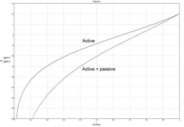
Figure 13.27 Baxandall active volume and active + passive control laws.
This arrangement is also free from pot dependence, so the gain depends only on the angular setting of the ganged control. However, this will no longer hold if the wiper of the final passive pot is significantly loaded. In practice, a high-input-impedance output buffer stage will be required, and this compromises the “zero noise at zero volume” property. On the other hand, a unity-gain buffer opamp is working in the best possible conditions for low noise, having no feedback resistors to introduce Johnson noise or convert opamp current noise to voltage noise. The source impedance for the buffer is usually non-zero, as it is fed from the wiper of the passive pot, but this can be made low in value, as the multiple inverting amplifiers in the Baxandall stage give plenty of drive capability. The passive pot does not have to be directly after the active volume control; intermediate stages could be inserted if required, giving a distributed volume control.
I have to say this idea is not exactly brand new. I first used it in consultancy work in, I think, 1982.
A practical version of this arrangement is shown in Figure 13.28, where both pots are 2 kΩ. Making them different in value would introduce some unwelcome complications in component sourcing, but such a custom component could be specified if there was a powerful reason to do so (which, as far as I can see, there isn’t).

In this case, a three-path Baxandall control is used, which has in itself an intermediate noise performance between the two-path and four-path versions in Table 13.4. There is some more discussion of this approach in Self On Audio. [7], [8]
While this technique gives a good volume law (and I have done quite a bit of knob-twiddling listening to confirm that), it does have some disadvantages. The extra expense of a four-gang pot is obvious, but there is another drawback which is slightly less so.
As noted, the great advantage of an active gain control is that it only provides the amount of gain required. However, we have now added a stage of passive attenuation, so there will be some impairment of headroom. Assume that in the circuit of Figure 13.28, the volume control is set for unity total gain, a control setting of Mark 7.5; the active Baxandall stage will have a gain of +2.4 dB, while the passive section will be attenuating by –2.4 dB. Therefore, 2.4 dB of headroom is lost in the final attenuator.
The Overlap Penalty
Obviously we would like to tailor the gain and attenuation laws so that the loss of headroom is as small as possible and exists over as small a range of volume settings as possible. The obvious way to do this is to arrange the gain law of the output attenuator so that as we turn down the volume, it does not introduce any attenuation until the Baxandall stage has reached unity gain. The difference between this ideal state and reality (such as Figure 13.28) I call the Overlap Penalty, as it results from the gain law overlapping with the attenuation law. It has nothing to do with the game of soccer or the arcane provisions of its offside rule. See Chapter 8 for another example.
However, we are limited to linear pots if we want to eliminate pot-dependency and retain channel matching that is as accurate as mechanical alignment permits. The Baxandall stage has its law fixed by its maximum gain and nothing else. Likewise, to avoid pot dependency, we cannot start pulling about the law of the output attenuator by adding fixed resistors. (It is assumed in Figure 13.28 that RV2 faces an input impedance that is very high compared with the pot track resistance and so is unloaded.) Therefore, it is hard to see what can be done.
Or is it? The obvious and expensive solution is to replace both the pots in Figure 13.28 with switched resistor ladders, as described later in this chapter. The Baxandall stage and the output attenuator can then have whatever law you can think up, and it is straightforward to arrange things so the output attenuator is only attenuating when the Baxandall stage has unity gain or less. I designed a rather advanced preamplifier using this method with four ganged 48-way switch wafers, actuated by either a stepper motor or a manual knob. Since one position really MUST be used as a mechanical stop, to avoid traumatic lurches from silence to full volume, we are left with 47 volume positions. Both the Baxandall and output attenuator ladders were composed of 47 Ω resistors to emulate linear pots, and no attempt was made to tweak the overall volume law. It seems to work very nicely as it is. This gave a total resistance in the Baxandall ladder of 2162 Ω and in the output attenuator 1410 Ω; there are fewer resistors in the latter because its top half does not attenuate, and the switch contacts there are simply wired together. These values are an implementation of low-impedance design and gave pleasingly low noise.
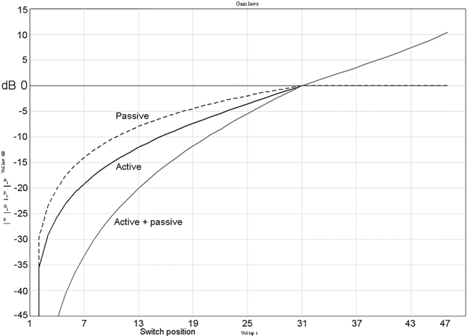
Figure 13.29 demonstrates how this method works. Above position 31, where the overall gain is unity, the “passive” curve stays at 0 dB. Therefore the “active” and “active+ passive” curves are the same and overlaid in the diagram. Below position 31, the passive output attenuator begins to act, improving the volume control law and giving the much-desired condition of zero noise out at zero volume.
Or does it? As the design stands, the output is taken directly from the moving contact of the output attenuator. The maximum output impedance of 329 Ω occurs at position 17, halfway down the resistor ladder, as expected. (Not halfway down the control travel, because the top half consists of links.) Such a resistance produces Johnson noise at -126.9 dBu (usual conditions), which is not quite zero but will be negligible compared with the overall noise performance.
While this is a reasonably low output impedance, it is rather greater than the usual 47 Ω or 56 Ω recommended in this book and would not be suitable for driving long cables. To reduce it, an output buffer is necessary, which will introduce noise of its own that cannot be turned down to zero. This could be a zero-impedance buffer, as described in Chapter 19. The output is of course unbalanced; if a balanced output is required, then both an output buffer and an inverter will be needed, with further compromise on the zero-volume noise floor.
Let’s put some numbers to this. In the preamplifier just above the output noise at zero volume measured -119.4 dBu (usual conditions) with the Audio Precision noise subtracted. Adding a unity-gain output buffer in the form of a 5532/2 voltage-follower increased this only to -116.8 dBu, which I hope you will agree is still extremely quiet. This is because a voltage-follower gives only the voltage noise of the opamp. A shunt-mode 5532/2 inverter with 1 kΩ input and feedback resistors was further added, driven from the output buffer to avoid loading on the output attenuator, to give a balanced output. The output noise was then measured between the hot output and the cold (inverted) output and -111.8 dBu obtained. This is not quite so good and stems from the 2-times noise gain of the inverter and the opamp current noise flowing in the input and feedback resistors. This is still very quiet indeed, and it is good to know that supplying a low (or zero) impedance output or a balanced output does not make a nonsense of having a very low-noise volume control system.
A quadruple bank of 48-way switches may be a near-perfect volume control in many ways, but it is unquestionably expensive. I began to wonder if there might be a way to produce suitably non-overlapping control laws using pots; the saving would be immense.
One possibility to consider was the use of the special balance-control pots that have one half of the track made of metal (giving no attenuation) and the other a standard resistive track; these are easily available, but the resistive track is usually a log-law, so balance accuracy may not be great. I am assuming here that you can separately specify that the active section of the quadpot has a standard linear law, or the active section will not work properly; a greater difficulty may be finding a balance control with linear resistive track and a suitably low resistance such as 1 kΩ. This method is illustrated in Figure 13.30. Having special pots made up of standard resistive tracks is usually not too much of a problem. Requests for non-standard tracks are, however, unlikely to be well received unless you promise to buy thousands.

Figure 13.30 Baxandall active volume plus two pot-based methods for eliminating the Overlap Penalty.
If suitable balance-control pots cannot be sourced, another possibility is to use centre-tapped pots. If you take a 2 kΩ centre-tapped pot and connect the tap to the top of the track, you have (up to a point) emulated a 1 kΩ pot where the top half causes no attenuation. A snag is that the output impedance of the output attenuator is now no longer zero for all the upper half of its travel. The maximum output impedance now occurs with the wiper 3/4 of the way up and is therefore a quarter of 1 kΩ, which is 250 Ω. In the lower half of wiper travel, the maximum output impedance is likewise 250 Ω at 1/4 of the way up. This is less than the 329 Ω maximum impedance given by the 48-position switched version and is unlikely to cause noise difficulties. This method is also illustrated in Figure 13.30.
In both cases, the gain of the active stage should ideally be unity with the volume control at midpoint (Mark 5) to eliminate the Overlap Penalty. I’ll say right away that I have not tried out either idea in practice due to the difficulty of obtaining one-off samples of odd pots.
Potentiometers and DC
As noted in the previous section, it is never a good idea to have DC flowing through any part of a potentiometer. If there is a DC voltage between the ends of the pot track, there will be rustling noises generated as the wiper moves up and down over minor irregularities in track resistance.
Feeding a bias current through a wiper to the next stage tends to create more serious noise because the variations in wiper contact resistance are greater. This tends to get worse as the track surface becomes worn. This practice is often acceptable for FET input op amps like the TL072, but it is definitely not a good idea for bipolar op amps such as the 5532, because the bias current is much greater, and so therefore is the noise on wiper movement. AC coupling is essential when using bipolar opamps. If you are using electrolytic capacitors, then make sure that the coupling time-constant is long enough for capacitor distortion to be avoided; see Chapter 2.
Belt-Ganged Volume Controls
Sometimes, if you want to use a particular fancy type of pot for volume control, you will find that dual versions for stereo are not available. One solution to this is to gang two pots together using toothed belts; it has been done. A possibly more extreme example is the Ayre AX-6 integrated amplifier [9], [10], which has two big Shallco switches (one for each channel) ganged by a toothed belt that is driven by a stepper motor, which is in turn controlled by a front panel rotary encoder. It is quoted as having 46 steps of volume control, suggesting a 48-position switch is being used, with presumably one position for a mechanical stop and one for “off”, i.e. infinite attenuation or near enough.
The belt-coupled concept would be valid with pot-based volume controls, but will it be accurate enough for good channel balance? When you consider that the printheads on inkjet and dot matrix printers all use toothed belts and achieve dot-placement accuracy better than a few thousandths of an inch all the time, it looks reasonably promising. It might not be quite as good as having two pots on the same solid shaft.
A rather crude way of ganging pots together with wooden levers was presented in Electronics World in 2002. [11] I do not feel this is a promising route to pursue.
Motorised Potentiometers
Motorised pots are simply ordinary pots driven by an attached electric motor, heavily geared down and connected to the control shaft through a silicone slipping clutch. This clutch allows manual adjustment of the volume when the motor is off and prevents the motor stalling when the pot hits the end of its travel; limit switches are not normally used. Motorised pots are now considerably cheaper than they used to be due to the manufacture of components in China that represent a very sincere homage to designs by ALPS and others, and they appear in lower- to middle-range integrated amplifiers. Motorisation can be added to any control that uses a rotary pot.
In many ways, they are the ideal way to implement a remote-controlled volume function. There is no variable gain electronics to add noise and distortion, manual control is always available if you can’t find the remote (so-called because it is never to hand), and the volume setting is inherently non-volatile, as the knob stays where it was left when you switch off.
A disadvantage is that the “feel” of a motorised pot is pretty certain to be worse than a normal control because of the need for the slipping clutch between the control shaft and the motor; a large-diameter weighted knob helps with this. The channel balance is of course no better than if the same pot was used as a manual control.
Since the motor has to be able to run in either direction, and it is simplest to run it from a single supply, an H-bridge configuration, as shown in Figure 13.31, is used to drive it. Normally all four transistors are off. To run the motor in one direction, Q1 and Q4 are turned on; to run in the other direction, Q2 and Q3 are turned on. The H-bridge and associated logic to interface with a microcontroller can be obtained in convenient ICs such as the BA6218 by Rohm. This IC can supply an output current of up to 700 mA. Two logic inputs allow four output modes: forward, reverse, idle (all H-bridge transistors off), and dynamic braking (motor shorted via ground). The logic section prevents input combinations that would turn on all four devices in the H-bridge and create (briefly) electronic mayhem.
The absence of limit switches means that if continuous rotation is commanded (for example, by sitting on the remote), there is the potential for the motor to overheat. It is a wise precaution to write the software so that the motor is never energised for longer than it takes to get from one extreme of rotation to the other, plus a suitable safety margin.

Figure 13.31 Control circuitry for a motorised volume control.
It would appear that there might be problems with electrical noise from the motor getting into the audio circuitry, but I have not myself found this to be a problem. In the usual version, the motor is screened with a layer of what appears to be GOSS (grain-oriented silicon steel) to keep magnetic effects under control, and the motor terminals are a long way from the audio terminals. A 100 nF capacitor across the motor terminals, and as close to them as practicable is always a good idea. (It is a fact that GOSS was invented by Dr Norman P. Goss.) The motor should be driven from a separate non-audio supply unless you’re really looking for trouble; motorised controls with 5 V motors are popular, as they can run off the same +5 V rail as a housekeeping microcontroller. I have never had problems with motor noise interfering with a microcontroller.
Linear faders, as used on mixing consoles, are also sometimes motorised, not for remote control, but to allow previously stored fader movements to be played back in an automatic mixdown system. A linear servo track next to the audio track allows accurate positioning of the fader. Motorisation has usually been done by adding a small electric motor to one end of the fader and moving the control knob through a mechanism of strings and pulleys that is strongly reminiscent of an old radio dial. Such arrangements have not always been as reliable as one might have hoped.
Stepped Volume Controls
The great feature of potentiometer-based volume controls is that they have effectively infinite resolution, so you can set exactly the level you require. If, however, you are prepared to forego this and accept a volume control that changes in steps, a good number of new possibilities open up and, in return, promise much greater law accuracy and channel balance. The technologies available include rotary-switched resistive attenuators, relay-switched resistive attenuators, switched multi-tap transformers, and specialised volume-control ICs. These options are examined in what follows.
The obvious question is: how small a step is needed to give satisfactory control? If the steps are made small enough, say less than 0.2 dB, they are imperceptible, always providing there are no switching transients, but there are powerful economic reasons for not using more steps than necessary. 2 dB steps are widely considered acceptable for in-car entertainment (implemented by an IC), but my view is that serious hi-fi requires 1 dB steps.
I have designed several power amplifiers with a switch that introduces 20 dB of attenuation. Its main use is to give a set-up mode so that level errors with powerful amplifiers do not cause smoking loudspeakers. If you are using a standard Baxandall active volume control with its rather flat law, the attenuation switch can also be used to move operation to a more favourable part of the law curve.
Switched Attenuator Volume Controls
For high-end products in which the imperfections of a ganged-potentiometer volume control are not acceptable, much superior accuracy can be achieved by using switched attenuators to control level. It is well known that the BBC for many years used rotary faders that were stud-switched attenuators working in 2 dB steps; some of these were still in use in 1961.
The normal practice is to have a large rotary switch that selects a tap on a resistor ladder; since the ladder can be made of 1% tolerance components, the channel matching is much better than that of the common dual-gang pot. A stereo control naturally requires two resistor ladders and a two-pole switch. The snag is of course the much greater cost; this depends to a large extent on how many control steps are used. The resistor ladders are not too costly unless exotic super-precision parts are used, but two-pole switches with many ways are neither cheap nor easy to obtain.
At the time of writing, one commercial preamp offers twelve 5 dB steps; the component cost has been kept down by using separate switches for left and right channels, which is not exactly a triumph of ergonomics. Another commercial product has an 11-position ganged switched attenuator. In my opinion, neither offers anything like enough steps.
The largest switches readily available are made up from 1 Pole 12-way wafers. The most common version has a Break before Make action, but this causes clicky transients due to the interruption of the audio waveform. Make before Break versions can usually be obtained, and these are much more satisfactory as the level changes, as the switch is rotated are much smaller, and the transients correspondingly less obtrusive. Make sure no circuitry gets overloaded when the switch is bridging two contacts.
Moving beyond 12-way, a relatively popular component for this sort of thing is a 24-position switch from the ELMA 04 range; this seems to be the largest number of ways they produce. A bit of care is needed in selecting the part required, as one version has 10 µm of silver on the contacts with a protective layer of only 0.2 µm-thick gold. This very thin layer is for protection during storage and transport only and in use will wear off quite quickly, exposing the silver, which is then subject to tarnishing, with the production of non-conductive silver sulphide; this version should be avoided unless used in a sealed environment. Other versions of these switches have thick 3 µm gold on the contacts, which is much more satisfactory. They can be obtained with one, two, or four 24-way wafers, but they are not cheap. At the time of writing (Jan 2009) two-wafer versions are being advertised by third parties at about $130 each, which means that in almost all cases the volume switch is going to cost a lot more than the rest of the preamplifier put together.
If 24 positions are not enough (which in my view is the case), 48-way switches are available from ELMA and Seiden, though in practice, they have to be operated as 47-way because the mechanical stop takes up one position. This stop is essential, as a sudden transition from silence to maximum volume is rarely a good idea. Fifty-eight-way switches are also available from Seiden. Shallco make switches with up to 48 positions in one-, two-, three-, and four-pole formats, but their specs say this only gives 24 non-shorting (break-before-make) positions. It seems to be essentially a make-before-break product line, and this may complicate or simplify switched volume-control design depending on how you are doing it. [12]
A switched attenuator can be made very low impedance to minimise its own Johnson noise and the effect of the current noise of the following stage. The limiting factors are that the attenuator input must present a load that can be driven with low distortion from the preceding stage and that the resistor values at the bottom of the ladder do not become too small for convenience. An impedance of around 1000 Ω from top to bottom is a reasonable choice. This means that the highest output impedance (which is at the–6 dB setting, a very high setting for a volume control) will be only 250 Ω. This has a Johnson noise of only -128.2 dBu (22 kHz bandwidth, 25°C) and is unlikely to contribute much to the noise output of a system. The choice of around 1000 Ω does assume that your chosen range of resistors goes down to 1 Ω rather than stopping at 10 Ω, though if necessary, the lower values can of course be obtained by paralleling resistors.
Assuming you want to use a 12-way switch, a possible approach is to use 12 steps of 4 dB each, covering the range 0 to -44 dB. My view is that such steps are too large, and 2 dB is much more usable, but you may not want to spend a fortune on a rotary switch with more ways. In fact, 1 dB steps are really required so you can always get exactly the volume you want, but implementing this with a single rotary switch is going to be very difficult, as it implies something like a 60- or 70-way switch. My current preamplifier just happens to be a relay-switched Cambridge Audio 840E with some 90-odd 1 dB steps.
There is no reason why the steps have to be equal in size, and it could be argued that the steps should be smaller around the centre of the range and larger at top and bottom to give more resolution where the volume control is most likely to be used. It does not really matter if the steps are not exactly equal; the vital thing is that they should be identical for the left and right channels to avoid image shift.
Figure 13.32a shows a typical switched attenuator of this sort, with theoretically exact resistor values; the size of each step is 4.00000 dB, accurate to five decimal places. In view of resistor tolerances, such accuracy may appear pretty pointless, apart from the warm feeling it produces, but it costs nothing to start off with more accuracy than you need. The total resistance of the ladder is 1057 Ω, which is a very reasonable load on a preceding stage, so long as it is implemented with a 5532, LM4562, or similar.
A lot depends on what range of resistor values you have access to. When I began to design preamplifiers, E12 resistors (12 values per decade) were the norm, and E24 resistors (24 values per decade) were rather rare and expensive. This is no longer the case, and E24 is freely available. Figure 13.32b shows the same attenuator with the nearest E24 value used for each resistor. The attenuation at each tap is still very accurate, the error never exceeding 0.12 dB except for the last tap, which is 0.25 dB high; this could be cured by making R12 a parallel combination of 6.8 Ω and 330 Ω and making R11 3.9 Ω, which reduces the last-tap error to 0.08 dB. To reduce the effect of tolerances R12 would be better made from two near-equal components; 12 Ω in parallel with 15 Ω is only 0.060% high in value.
The next most prolific resistor range is E96, with no less than 96 values in a decade –nobody seems interested in making an E48 range as such, though it is of course just a sub-set of E96. Using the nearest E96 value in the attenuator, we get Figure 13.32c, where the taps are accurate to within 0.04 dB; remember that this assumes that each resistor is exactly the value it should be and does not incorporate any tolerances. The improvement in accuracy is not enormous, and if you can get a tighter tolerance in the E24 range than E96, E24 is the preferred option.
There is also an E192 resistor range, but it is rather rare, and there seems to be no pressing need to use so many different values in volume control attenuators.
Almost all the work in the design of a switched attenuator is the calculation of the resistor values in the ladder. Putting in likely component values and attempting to tweak them by hand is a most unpromising approach, because all the values interact, and you will boil off your sanity. A systematic spreadsheet approach is the only way. This is probably the simplest:
- Decide the approximate total resistance of the resistor ladder.
- Decide the step size, say 4 dB.
- Take a two-resistor potential divider, where the sum of the resistors equals the desired total resistance, and choose exact values for a 4 dB attenuation; use the goal-seek tool to get the exact value for the bottom resistor. (An exact E24 value at the top of the ladder is not essential, but it is convenient.)
- Now split the bottom resistor into two, so that another 4 dB attenuator results. Check that the attenuation really is correct, because an error will propagate through the rest of the process, and you will have to go back and do it all again from that point. Repeat this step until you have enough resistors in the ladder for the number of taps required.
- When the table of resistor values is complete, for each resistor, pick the nearest value from the E-series you are using. Alternatively, select a parallel pair to get closer to the desired value, keeping the two resistors as near equal as possible.
You will then have constructed something like the spreadsheet shown in Table 13.7, which gives the E24 resistor values shown in Figure 13.32b. The chosen value at the top of the ladder is 390 Ω. The spreadsheet has been set up to give more information than just the resistor value and the tap attenuation; it gives the voltage at each tap for a given input (10 V in this case) in column 5, the output impedance of each tap in column 6, the step size in dB in column 8, and the absolute error for each tap in column 9. It also gives the total resistance of the ladder, the current through it for the specified input voltage, and the resulting power dissipation in each resistor in column 7. The last parameter is unlikely to be a major concern in an audio attenuator, but if you’re working with very low impedances to minimise noise, it is worth keeping an eye on.

Before the design work begins, you must consider the stages before and after the attenuator. It is strongly recommended that the attenuator input is driven from a very low impedance such as the output of an opamp with plenty of negative feedback so the source impedance can be effectively considered as zero and does not enter into the calculations. The loading on the output of the attenuator is more of a problem. You can either take loading on the output into account in the calculations, in which case the shunting effect of the load must be incorporated into step 3), or else make the input impedance of the next stage so high that it has a negligible effect.
As an example, the E24 network in Figure 13.32b was calculated with no allowance for loading on the output. Its highest output impedance is 253 Ω at Tap 3, so this is the worst case for both loading-sensitivity and noise. If a load of 100 kΩ is added, the level at this tap is pulled down by only 0.022 dB. A 100 kΩ input impedance for a following stage is easy to arrange, so the extra computation required in allowing for loading is probably not worthwhile unless for some very good reason the loading is much heavier. The Johnson noise of 253 Ω is still only -128.2 dBu.
If you feel you can afford 24-way switches, then there is rather more flexibility in design. You could cover from 0 to –46 dB in 2 dB steps, 0 to –57.5 dB in 2.5 dB steps, or 0 to -69 dB in 3 dB steps. There are infinite possibilities for adopting varying step sizes.
Table 13.8 shows the resistor values for 0 to –46 dB in 2 dB steps, Table 13.9 gives those for 0 to –57.5 dB in 2.5 dB steps, and Table 13.10 gives the values for 0 to -69 dB in 3 dB steps. All three tables give the nearest E24 and E96 values and the resulting errors. Note the first two versions start off with a 220 Ω resistor at the top, but on moving from 2 dB to 2.5 dB steps, the resistors towards the bottom naturally get smaller to give the greater attenuation required, and the total ladder resistance falls from 1060 Ω to 866 Ω. To prevent the resistor values becoming inconveniently small and the total resistance too low, the 3 dB-step version starts off with a higher value resistor of 430 Ω at the top; this increases the total resistance of the ladder to 1470 Ω and raises the maximum output impedance to 368 Ω at Tap 3. The Johnson noise of 368 Ω is naturally higher at -126.5 dBu, but this is still very low compared with the likely noise from amplifier stages downstream.
The exact values on the left hand of each table can be scaled to give the total divider resistance required, but it will then be necessary to select the nearest E24 or E96 value manually. If you are increasing all the resistances by a factor of 10, then the same E24 or E96 values with a zero added can be used. The average of the absolute error for all 24 steps is shown at the bottom of each section; note that simply taking the average error would give a misleadingly optimistic result because the errors are of random sign and would partially cancel.
| 1 | 2 | 3 | 4 | 5 | 6 | 7 | 8 | 9 | 10 |
|---|---|---|---|---|---|---|---|---|---|
| Nearest E24 value | Divider Current= |
0.0096 | Amps rms |
||||||
| INPUT= | 10 | Vrms | Total res= | 1046.6 | |||||
| dB Ref= | 0 | ||||||||
| Tap Z | Step | Tap error | Tap No. | ||||||
| Ohms | ratio | dB | O/P V | Ohms | Power mW | dB | dB | 1 | |
| R1 | 390 | 35.6 | |||||||
| 0.62736 | –4.050 | 6.2736 | 244.672 | 4.0496 | –0.0496 | 2 | |||
| R2 | 240 | 21.9 | |||||||
| 0.39805 | –8.001 | 3.9805 | 250.77 | 3.952 | –0.0012 | 3 | |||
| R3 | 150 | 13.7 | |||||||
| 0.25473 | –11.878 | 2.5473 | 198.69 | 3.877 | 0.1216 | 4 | |||
| R4 | 100 | 9.1 | |||||||
| 0.15918 | –15.962 | 1.5918 | 140.08 | 4.084 | 0.0379 | 5 | |||
| R5 | 62 | 5.7 | |||||||
| 0.09994 | –20.005 | 0.9994 | 94.15 | 4.043 | –0.0050 | 6 | |||
| R6 | 39 | 3.6 | |||||||
| 0.06268 | –24.058 | 0.6268 | 61.49 | 4.053 | –0.0575 | 7 | |||
| R7 | 24 | 2.2 | |||||||
| 0.03975 | –28.014 | 0.3975 | 39.95 | 3.956 | –0.0137 | 8 | |||
| R8 | 15 | 1.4 | |||||||
| 0.02542 | –31.898 | 0.2542 | 25.92 | 3.884 | 0.1020 | 9 | |||
| R9 | 10 | 0.9 | |||||||
| 0.01586 | –35.993 | 0.1586 | 16.34 | 4.095 | 0.0065 | 10 | |||
| R10 | 6.2 | 0.6 | |||||||
| 0.00994 | –40.055 | 0.0994 | 10.30 | 4.061 | –0.0549 | 11 | |||
| R11 | 3.6 | 0.3 | |||||||
| 0.00650 | –43.745 | 0.0650 | 6.76 | 3.690 | 0.2546 | 12 | |||
| R12 | 6.8 | 0.6 |
| Switched attenuator: 2 dB steps | |||||||||
|---|---|---|---|---|---|---|---|---|---|
| Exact | Using E24 values | Using E96 values | |||||||
|
Tap |
Ohms |
Step
dB |
Ohms |
Step
dB |
Error
dB |
Ohms |
Step
dB |
Error
dB |
|
| 1 | R1 | 220.0000 | 0.0000 | 220 | 0.0000 | 0.0000 | 220 | 0.0000 | 0.0000 |
| 2 | R2 | 174.7490 | –2.0000 | 180 | –2.0435 | –0.0435 | 174 | –2.0208 | –0.0208 |
| 3 | R3 | 138.8080 | –4.0000 | 130 | –4.1427 | –0.1427 | 137 | –4.0114 | –0.0114 |
| 4 | R4 | 110.2591 | –6.0000 | 110 | –6.0660 | –0.0660 | 110 | –5.9942 | 0.0058 |
| 5 | R5 | 87.5819 | –8.0000 | 82 | –8.1104 | –0.1104 | 86.6 | –7.9967 | 0.0033 |
| 6 | R6 | 69.5688 | –10.0000 | 68 | –10.0251 | –0.0251 | 69.8 | –9.9799 | 0.0201 |
| 7 | R7 | 55.2605 | –12.0000 | 56 | –12.0124 | –0.0124 | 54.9 | –11.9914 | 0.0086 |
| 8 | R8 | 43.8950 | –14.0000 | 43 | –14.0788 | –0.0788 | 44.2 | –13.9838 | 0.0162 |
| 9 | R9 | 34.8670 | –16.0000 | 33 | –16.0850 | –0.0850 | 34.8 | –16.0046 | –0.0046 |
| 10 | R10 | 27.6958 | –18.0000 | 27 | –18.0166 | –0.0166 | 27.4 | –18.0107 | –0.0107 |
| 11 | R11 | 22.0000 | –20.0000 | 22 | –19.9959 | 0.0041 | 22.0 | –19.9987 | 0.0013 |
| 12 | R12 | 17.4749 | –22.0000 | 18 | –22.0272 | –0.0272 | 17.4 | –22.0077 | –0.0077 |
| 13 | R13 | 13.8808 | –24.0000 | 13 | –24.1361 | –0.1361 | 13.7 | –24.0093 | –0.0093 |
| 14 | R14 | 11.0259 | –26.0000 | 11 | –26.0577 | –0.0577 | 11.0 | –25.9916 | 0.0084 |
| 15 | R15 | 8.7582 | –28.0000 | 8.2 | –28.1000 | –0.1000 | 8.66 | –27.9934 | 0.0066 |
| 16 | R16 | 6.9569 | –30.0001 | 6.8 | –30.0120 | –0.0120 | 6.98 | –29.9758 | 0.0242 |
| 17 | R17 | 5.5260 | –32.0001 | 5.6 | –31.9960 | 0.0040 | 5.49 | –31.9863 | 0.0137 |
| 18 | R18 | 4.3895 | –34.0001 | 4.3 | –34.0580 | –0.0580 | 4.42 | –33.9773 | 0.0227 |
| 19 | R19 | 3.4867 | –36.0001 | 3.3 | –36.0588 | –0.0588 | 3.48 | –35.9964 | 0.0036 |
| 20 | R20 | 2.7696 | –38.0001 | 2.7 | –37.9839 | 0.0161 | 2.74 | –38.0004 | –0.0004 |
| 21 | R21 | 2.1999 | –40.0001 | 2.2 | –39.9548 | 0.0452 | 2.20 | –39.9857 | 0.0143 |
| 22 | R22 | 1.7475 | –42.0000 | 1.8 | –41.9753 | 0.0247 | 1.74 | –41.9913 | 0.0087 |
| 23 | R23 | 1.3881 | –44.0000 | 1.5 | –44.0701 | –0.0701 | 1.37 | –43.9886 | 0.0114 |
| 24 | R24 | 5.3609 | –46.0001 | 5.1 | –46.3095 | –0.3095 | 5.36 | –45.9657 | 0.0343 |
| Total res= | 1055 | Ω | Total res= | 1065 | Ω | ||||
| Avg abs error= | 0.0654 | dB | Avg abs error= | 0.0117 | dB | ||||
| Switched attenuator: 2.5 dB steps | |||||||||
|---|---|---|---|---|---|---|---|---|---|
| Exact | Using E24 values | Using E96 values | |||||||
|
Tap |
Ohms |
Step
dB |
Ohms |
Step
dB |
Error
dB |
Ohms |
Step
dB |
Error
dB |
|
| 1 | R1 | 220.0000 | 0.0000 | 220 | 0.0000 | 0.0000 | 220 | 0.0000 | 0.0000 |
| 2 | R2 | 164.9809 | –2.4999 | 160 | –2.5471 | –0.0471 | 165 | –2.4997 | 0.0003 |
| 3 | R3 | 123.7182 | –4.9999 | 120 | –5.0208 | –0.0208 | 124 | –4.9907 | 0.0093 |
| 4 | R4 | 92.7756 | –7.4999 | 91 | –7.4864 | 0.0136 | 93.1 | –7.4901 | 0.0099 |
| 5 | R5 | 69.5719 | –10.0000 | 68 | –9.9726 | 0.0274 | 69.8 | –9.9928 | 0.0072 |
| 6 | R6 | 52.1715 | –12.5000 | 51 | –12.4441 | 0.0559 | 52.3 | –12.4958 | 0.0042 |
| 7 | R7 | 39.1231 | –15.0000 | 39 | –14.9066 | 0.0934 | 39.2 | –14.9974 | 0.0026 |
| 8 | R8 | 29.3382 | –17.5000 | 30 | –17.4130 | 0.0870 | 29.4 | –17.4982 | 0.0018 |
| 9 | R9 | 22.0005 | –20.0000 | 22 | –19.9969 | 0.0031 | 22 | –19.9995 | 0.0005 |
| 10 | R10 | 16.4981 | –22.5000 | 16 | –22.5429 | –0.0429 | 16.5 | –22.4952 | 0.0048 |
| 11 | R11 | 12.3718 | –25.0000 | 12 | –25.0153 | –0.0153 | 12.4 | –24.9899 | 0.0101 |
| 12 | R12 | 9.2775 | –27.5000 | 9.1 | –27.4790 | 0.0210 | 9.31 | –27.4890 | 0.0110 |
| 13 | R13 | 6.9572 | –30.0000 | 6.8 | –29.9627 | 0.0373 | 6.98 | –29.9914 | 0.0086 |
| 14 | R14 | 5.2172 | –32.5000 | 5.1 | –32.4310 | 0.0690 | 5.23 | –32.4939 | 0.0061 |
| 15 | R15 | 3.9123 | –35.0000 | 3.9 | –34.8893 | 0.1107 | 3.92 | –34.9949 | 0.0051 |
| 16 | R16 | 2.9338 | –37.5000 | 3.0 | –37.3900 | 0.1100 | 2.94 | –37.4948 | 0.0052 |
| 17 | R17 | 2.2000 | –40.0000 | 2.2 | –39.9658 | 0.0342 | 2.2 | –39.9950 | 0.0050 |
| 18 | R18 | 1.6498 | –42.5000 | 1.6 | –42.5014 | –0.0014 | 1.65 | –42.4892 | 0.0108 |
| 19 | R19 | 1.2372 | –45.0000 | 1.2 | –44.9601 | 0.0399 | 1.24 | –44.9818 | 0.0182 |
| 20 | R20 | 0.9277 | –47.5001 | 0.91 | –47.4057 | 0.0943 | 0.931 | –47.4783 | 0.0217 |
| 21 | R21 | 0.6957 | –49.9999 | 0.68 | –49.8653 | 0.1347 | 0.698 | –49.9771 | 0.0229 |
| 22 | R22 | 0.5217 | –52.4999 | 0.51 | –52.3019 | 0.1981 | 0.523 | –52.4748 | 0.0252 |
| 23 | R23 | 0.3912 | –54.9997 | 0.39 | –54.7183 | 0.2817 | 0.392 | –54.9694 | 0.0306 |
| 24 | R24 | 1.1731 | –57.4997 | 1.20 | –57.1626 | 0.3374 | 1.18 | –57.4608 | 0.0392 |
| Total res= | 866 | Ω | Total res= | 881 | Ω | ||||
| Avg abs error= | 0.0816 | dB | Avg abs error= | 0.0113 | dB | ||||
| Switched attenuator: 3 dB steps | |||||||||
|---|---|---|---|---|---|---|---|---|---|
| Exact | Using E24 values | Using E96 values | |||||||
|
Tap |
Ohms |
Step
dB |
Ohms |
Step
dB |
Error
dB |
Ohms |
Step
dB |
Error
dB |
|
| 1 | R1 | 430.0000 | 0.0000 | 430 | 0.0000 | 0.0000 | 430 | 0.0000 | 0.0000 |
| 2 | R2 | 304.4210 | –3.0000 | 300 | –2.9981 | 0.0019 | 301 | –3.0066 | –0.0066 |
| 3 | R3 | 215.5135 | –6.0000 | 220 | –5.9437 | 0.0563 | 215 | –5.9727 | 0.0273 |
| 4 | R4 | 152.5719 | –9.0000 | 150 | –8.9930 | 0.0070 | 154 | –8.9583 | 0.0417 |
| 5 | R5 | 108.0126 | –12.0000 | 110 | –11.9281 | 0.0719 | 107 | –11.9800 | 0.0200 |
| 6 | R6 | 76.4671 | –15.0000 | 75 | –14.9622 | 0.0378 | 76.8 | –14.9437 | 0.0563 |
| 7 | R7 | 54.1346 | –18.0000 | 56 | –17.8769 | 0.1231 | 54.9 | –17.9414 | 0.0586 |
| 8 | R8 | 38.3243 | –21.0000 | 39 | –20.9466 | 0.0534 | 38.3 | –20.9732 | 0.0268 |
| 9 | R9 | 27.1315 | –24.0000 | 27 | –23.9857 | 0.0143 | 27.4 | –23.9652 | 0.0348 |
| 10 | R10 | 19.2077 | –27.0000 | 20 | –26.9606 | 0.0394 | 19.1 | –26.9917 | 0.0083 |
| 11 | R11 | 13.5980 | –30.0000 | 13 | –30.0906 | –0.0906 | 13.7 | –29.9736 | 0.0264 |
| 12 | R12 | 9.6266 | –33.0000 | 10 | –32.9681 | 0.0319 | 9.53 | –32.9950 | 0.0050 |
| 13 | R13 | 6.8151 | –36.0000 | 6.8 | –36.0924 | –0.0924 | 6.81 | –35.9624 | 0.0376 |
| 14 | R14 | 4.8248 | –38.9999 | 4.7 | –39.1209 | –0.1209 | 4.87 | –38.9497 | 0.0503 |
| 15 | R15 | 3.4157 | –42.0000 | 3.3 | –42.0755 | –0.0755 | 3.40 | –41.9678 | 0.0322 |
| 16 | R16 | 2.4181 | –45.0000 | 2.4 | –44.9831 | 0.0169 | 2.43 | –44.9436 | 0.0564 |
| 17 | R17 | 1.7119 | –48.0000 | 1.8 | –47.9476 | 0.0524 | 1.74 | –47.9433 | 0.0567 |
| 18 | R18 | 1.2119 | –51.0001 | 1.2 | –51.1090 | –0.1090 | 1.21 | –50.9841 | 0.0159 |
| 19 | R19 | 0.8580 | –54.0001 | 0.82 | –54.1167 | –0.1167 | 0.866 | –53.9772 | 0.0228 |
| 20 | R20 | 0.6074 | –57.0002 | 0.62 | –57.0034 | –0.0034 | 0.604 | –57.0068 | –0.0068 |
| 21 | R21 | 0.4300 | –60.0003 | 0.43 | –60.0776 | –0.0776 | 0.432 | –59.9949 | 0.0051 |
| 22 | R22 | 0.3044 | –63.0003 | 0.30 | –63.1079 | –0.1079 | 0.301 | –63.0148 | –0.0148 |
| 23 | R23 | 0.2155 | –66.0003 | 0.22 | –66.0982 | –0.0982 | 0.215 | –65.9860 | 0.0140 |
| 24 | R24 | 0.5224 | –69.0003 | 0.51 | –69.2132 | –0.2132 | 0.523 | –68.9771 | 0.0229 |
| Total res= | 1473 | Ω | Total res= | 1470 | Ω | ||||
| Avg abs error= | 0.0701 | dB | Avg abs error= | 0.0281 | dB | ||||
If the available switches do not give enough steps, a possible solution is to use two rotary switches, one for coarse volume control and the other for vernier control, the latter perhaps in 1 dB steps or less. While straightforward to design, this is not exactly user friendly. A buffer stage is usually desirable to prevent the second attenuator from loading the first one; the second attenuator may present a constant load, but it is a heavy one. With no buffer, the total loading of the two attenuators could also present an excessive load to the stage before the first attenuator.
A rotary switch does not of course have the smooth feel of a good potentiometer. To mitigate this, a switched volume control may need a large-diameter weighted knob, possibly with some sort of silicone damping. Sharp detents and a small knob do not a good volume control make.
Relay-Switched Volume Controls
If you need more steps than a switch can provide, it is relatively simple to come up with a system that emulates a rotary switch with as many as desired, using relays, a microcontroller, and an inexpensive shaft encoder; you will need a relay for each step, and that will be an awful lot of relays. Another approach is to use relays in a ladder attenuator, which greatly reduces the relay count. This is dealt with in the next section. As soon as a microcontroller is introduced, then there is of course the possibility of infra-red remote control. The ultimate development in stepped volume controls is the relay ladder attenuator. This allows any number of steps to be employed.
The design of a ladder attenuator relay volume control is not quite as simple as it may appear. If you try to use a binary system, perhaps based on an R-2R network, you will quickly find that horrible transients erupt on moving from, say, 011111 to 100000. This is because relays have an operating time that is both long by perceptual standards and somewhat unpredictable. It is necessary to use logarithmic resistor networks with some quite subtle relay timing.
Currently, the highest expression of this technology is the Cambridge Audio 840A Integrated amplifier and 840E preamplifier. The latter uses second-generation relay volume control technology, using only 12 relays to give 1 dB steps over most of the control range. A rather unexpected feature of relay volume controls is that having purchased a very sophisticated preamplifier, where the precision relay control is the major unique feature, some customers then object to the sound of the relays clicking inside the box when they adjust the volume setting. You just can’t please some people.
Transformer-Tap Volume Controls
There are other ways of controlling volume than with resistors. At the time of writing (2020), there is at least one passive preamplifier on the market that controls volume by changing the taps on the secondary of a transformer. The unit I have in mind has only 12 volume steps, apparently each of 4 dB. These are very coarse steps for a volume control –unacceptably so, I would have thought; a 48 dB range also seems too small. Some 24-way switches are available (see the section on switched attenuator volume controls), but they are expensive. There are several potential problems with this approach –transformers are well known to fall much further short of being an ideal component than most electronic parts do. They can introduce frequency response irregularities, LF distortion, and hum. They are relatively heavy and expensive, and the need for a large number of taps on the secondary puts the price up further. The multi-way switch to select the desired tap must also be paid for.
There are, however, some advantages. The output impedance of a resistive potential divider varies according to its setting, being a maximum at -6 dB. Assuming it is fed from a low impedance, a transformer volume control has a low impedance at every tap, greater than zero only by the resistance of the windings and handily lower than even a low-resistance pot. This gives lower Johnson noise and minimises the effect of the current noise of the following stage. The much-respected Sowter transformer company makes a large number of different volume-control transformers, of which the most representative is probably the 9335 model. This is basically a 1:1 transformer with taps on the secondary that give attenuation from 0 to -50 dB in 26 steps of 2 dB each. The DC resistance of both primary and secondary is 310 Ω. The total resistance of the windings is therefore 620 Ω, which is much lower than the value of the volume pots normally used. Note, however, that it is not much lower than the 1 kΩ pots I used in the Elektor preamplifier. [6] At the time of writing, 2020, the 9335s cost £160 each. You need two for stereo.
Integrated Circuit Volume Controls
Specialised volume-control ICs based on switched networks have been around for a long time but have only recently reached a level of development at which they can be used in high-quality audio. Early versions had problems with excessively large volume steps, poor distortion performance, and nasty glitching on step changing. The best contemporary ICs are greatly improved; a modern example is the PGA2310 from Burr-Brown (Texas Instruments), which offers two independent channels with a gain range from +31.5 to -95.5 dB in 0.5 dB steps and is spec’d at 0.0004% THD at 1 kHz for a 3 Vrms input level. The IC includes a zero crossing detection function intended to give noise-free level transitions. The concept is to change gain settings on a zero crossing of the input signal and so minimise audible glitches. Gain control is by means of a three-wire serial interface, which is normally driven by a rotary encoder and a microcontroller such as one of the PIC series. The Yamaha YAC523 has a similar specification but incorporates seven gain-controlled channels for AV applications.
A similar device is the Texas Instruments PGA2311; it is likewise stereo, and the main difference is that the analogue power supply is ±5 V rather than the ±15 V of the PGA2310, which must limit the headroom. At least one manufacturer uses both channels in parallel for lower noise, presumably 3 dB lower.
Volume ICs are available for operation off a single +5 V rail, allowing operation off a USB port, but the THD figures can be an order of magnitude worse than devices running from ±15 V. One example is the stereo MAX5486, which can run from a single +2.7 V to +5.5 V rail or dual ±2.7 V rails. Other low-voltage examples are the DS1669 digital potentiometer IC from Dallas Semiconductors and the M62429 from Renesas Electronics. [13] For suitable low-voltage opamps, see Chapter 5.
Loudness Controls
It is an awkward but inescapable feature of human hearing that its frequency response varies with the level of the sound. As the level drops, the perceived loudness of high and low frequencies falls faster than the middle frequencies. This is very clearly expressed by the well-known Fletcher and Munson curves [14], shown in Figure 13.33. Their work was repeated by Robinson and Dadson [15], whose results are sometimes considered to be more accurate and were the basis for the ISO equal-loudness curves. A great deal of information on these curves and the differences between them and on the whole subject of loudness controls can be found in JAES papers by Newcomb and Young [16] and Holman and Kampmann. [17] More on their work later.

The graph shows what sound pressure level above the threshold of hearing is needed to get a constant result in phons, the unit of subjective loudness. The first disconcerting feature is that none of the curves are remotely flat –at 20 Hz, the sensitivity of the ear is always much lower than at 1 kHz, no matter what the level. A vital point is that the slopes at the bass end increase as the level falls, as shown in Column 2 of Table 13.11, which gives the average slope in dB per octave between 20 and 100 Hz. At 20 phons, the slope is greater than that of a third order filter, while at 100 phons, it is less than that of a second-order filter.
| 1 | 2 | 3 | 4 |
|---|---|---|---|
| Loudness (phons) | Slope (dB/octave) | SPL at 20 Hz ref 1 kHz (dB) | SPL at 10 kHz ref 1 kHz (dB) |
| 100 | 10.7 | +28 | +6 |
| 90 | 11.6 | +30 | +5 |
| 80 | 12.5 | +34 | +5 |
| 70 | 13.4 | +37 | +5 |
| 60 | 14.7 | +42 | +5 |
| 50 | 15.1 | +46 | +8 |
| 40 | 16.8 | +50 | +9 |
| 30 | 17.7 | +57 | +10 |
| 20 | 18.6 | +61 | +10 |
| 10 | 20.3 | +68 | +9 |
This increase of slope means that if you have satisfactory reproduction at a given sound level, turning down the volume gives a subjective loss of bass, demonstrated by the increased SPLs required to get the same number of phons at 20 Hz in Column 3. There are also some complicated but much smaller variations in the treble (see Column 4). This effect used to be called “scale distortion” in the 1950s, which is a less-than-satisfactory term, not least because it sounds as if it would be of interest only to aquarists. At the time, there was intense debate as to whether attempting to compensate for it by making the frequency response vary with the volume control setting, turning it into what became called a “loudness control”, was the right thing to do or not. A switch to make the volume control into a loudness control was a common feature in the 1970s, though there was still much debate as to whether it was a useful approach, with hi-fi purists roundly condemning the notion. Loudness controls are currently out of fashion; if you’re the kind of person that won’t tolerate tone controls, you probably regard loudness controls as totally anathema. However, the wheel of fashion turns, and it is well worth looking at how they work.
Note that we are not trying to make the Fletcher and Munson curves flat. If we take the 100-phon level as an example, we would need some 42 dB of boost at 20 Hz, which is clearly not right. What we are trying to do is reduce the differences in perceived bass level with volume changes. Let us assume we have a “flat” subjective response at a level of 100 phons, since it roughly corresponds to 100 dB SPL, which is pretty loud, typically described as “jackhammer at 1 metre”. Figure 13.34 shows the correction response we would need to bring the lower levels into line with the 100-phon curve. This was obtained by subtracting the 100 phon data from that for the other levels. The curves look a little wobbly, as they cannot be read from the graph in Figure 13.33 with accuracy much better than 1 dB.
Clearly the correction shown above 1 kHz is neither large nor consistent. Holman and Kampmann state clearly that above 400 Hz correction is neither “necessary or desirable”. [18] Correction below 1 kHz, however, is a different matter. Fortunately, it consists of a monotonic curves, though they do have varying slopes. For the higher levels the hinge point between sloping and flat is around 600 Hz, increasing as the level falls to about 1 kHz. The slope, averaged between 20 Hz and 1 kHz, varies between 0.5 dB/octave at 90 phons to 7.3 dB/octave at 10 phons. If we assume that 10 phons is too low a level to worry about, we find the 20-phons correction curve has a slope of only 5.8 dB, which promises that we could implement a useful compensation network using only simple first-order circuitry.

The Fletcher and Munson curves depend on the absolute level at the ear, and this obviously depends on amplifier gain, loudspeaker efficiency, room acoustics, and many other factors. Unless you set up your system for a defined SPL which you regard as “flat”, loudness compensation is going to be a rather approximate business, and this is one argument frequently advanced against it.
Switchable loudness facilities were fitted to a large number of Japanese amplifiers in the 1970s and ’80s, but European and USA manufacturers rarely used them. The circuitry used was virtually standard, with three typical versions shown in Figure 13.35. With the loudness switch set to “OUT”, the capacitors do nothing, and we have a linear pot loaded down at its tap by R1 to approximate a logarithmic volume law. (I assume that the pot must be linear; Japanese service manuals seem remarkably coy about the law of the pot, and only in one case have I found it confirmed as linear.) When the loudness switch is set to “IN”, C1 gives HF boost, and C2 gives LF boost by reducing the loading effect of R1.

Figure 13.35 Three typical switchable loudness controls using a centre-tapped linear pot.
The simulated frequency response for the Denon circuit is shown in Figure 13.36. There are three notable features; first, there is a lot of boost applied at HF, despite the fact that, as we saw earlier, no HF correction is actually wanted. The second is that the correction curves only change in shape over the top half of the control rotation, the response being fixed below that. Third, there is a rather dramatic change in mid-band level between Marks 5 and 6 as the pot wiper approaches the centre-tap.
The almost universal inclusion of HF boost in these loudness circuits is a bit of a mystery. I can only assume that people took a quick look at the Fletcher and Munson curves and saw increases at the HF end but did not notice that the curves are essentially equally spaced, not varying in shape with level. I wonder if this unwanted HF boost was one of the reasons loudness controls were so poorly regarded; in their heyday, the primary source was vinyl, with bad distortion characteristics at HF. It seems likely that the HF boost would have accentuated this. For each of the three versions shown here, removing C1 removes the HF boost action.
These loudness controls must represent the widest-ever use of centre-tapped pots, which are otherwise rarely encountered. Pioneer used a centre-tapped pot with a simple loading resistor to ground connected to the tap to emulate a logarithmic law; there was no loudness facility. See the Pioneer A-88X and the A-77X (1985).
A few other loudness schemes were used. The Sansui A60 and A80 amplifiers had separate loudness and volume pots, making for cumbersome operation.

Figure 13.36 Frequency response of the Denon loudness control in Figure 13.35a. Complete pot rotation is from Marks 0–10; curve 0 not shown.
The Newcomb and Young Loudness Control
In 1976, Newcomb and Young published a very thoughtful paper on loudness controls. [16] They listed three important points about the Fletcher and Munson curves:
- There is little change in slope above 1 kHz. In other words, HF boost is not wanted, as I noted.
- The maximum LF boost required exceeds 6 dB/octave and cannot be provided by a single RC time-constant.
- The LF breakpoint moves upward in frequency as the SPL decreases.
To implement these three requirements, they put forward an ingenious active loudness control that compensated at LF only; see Figure 13.37. There is still a requirement to have a gain control as well in the signal path so the SPL can be aligned with the loudness control to get the compensation right.
Since RV1 alters both the input and feedback arms around A1, it gives a quasi-log volume law. The tolerance of the pot tracks will affect the channel balance accuracy, as unlike in the Baxandall volume control, the track resistance errors are not eliminated. The increased slope is implemented by C2 in conjunction with C3.
The resulting loudness curves are shown in Figure 13.38; the component values are as given by Newcomb and Young and are of rather higher impedance than I would use. The slope of the -40 dB curve is significantly greater than 6 dB/octave; between 20 and 40 Hz, it is 8 dB/octave. The first response breakpoint is set at an almost constant frequency by R2 and C2. The second -3 dB breakpoint moves up from 60 Hz at 0 dB loudness to 230 Hz at -40 dB loudness due to the action of RV1, R3, and C3. The maximum flat gain is set by R4. Note that the 200 nF capacitors are from the E24 series and so may be hard to source, and the value of R3 at 3k5 is not in any of the standard resistor series, including E96; the nearest E96 value is 3k48.
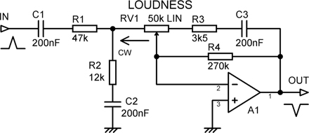

The presence of R2, which is effectively connected to ground at all but the lowest audio frequencies, increases the noise gain of the circuit, especially when loudness is set to maximum, when R2 is connected directly to the summing point at A1 inverting input. At maximum loudness, the noise gain is +15.1 dB, which is worryingly high; without R2, it would be only +5.8 dB. With R2 in place, the noise gain is still +4.8 dB at the middle loudness setting; see Table 13.12 for full details.
| Noise gain | Noise gain | |
|---|---|---|
| Control mark | x | dB |
| 10 | 5.671 | 15.073 |
| 9 | 3.824 | 11.650 |
| 8 | 2.915 | 9.294 |
| 7 | 2.372 | 7.502 |
| 6 | 2.008 | 6.056 |
| 5 | 1.746 | 4.841 |
| 4 | 1.546 | 3.787 |
| 3 | 1.389 | 2.851 |
| 2 | 1.259 | 2.003 |
| 1 | 1.151 | 1.222 |
| 0 | 1.058 | 0.490 |
The relatively high value resistors in the design, common for the period, will increase the effect of A1 current noise and will have high Johnson noise themselves. Reducing the values by low-impedance design should be straightforward, but changing the noise gain characteristics would require complete redesign. The circuit is ingenious, but both the noise gain and channel balance accuracy will need close examination.
In 1978, Holman and Kampmann put forward [17] an in-depth analysis of alternative loudness curves such as Robson and Dadson [15] and curves produced by Stevenson. They looked at the Newcomb and Young circuit; new component values for R2 and C2 were derived but not actually disclosed in the paper. Not sure how that got past peer review. Also, a linear attenuating pot was placed after the circuit, ganged with the loudness pot, to improve the control law.
Interest in loudness controls has pretty much been negligible since then.
References
[1] Baxandall, Peter “Audio Gain Controls” Wireless World, Nov 1980, pp 79–81
[2] Reiner, Rob (Director) This Is Spinal Tap. Film, 1984
[3] Self, Douglas “A Precision Preamplifier” Electronics World, Oct 1983
[4] Self, Douglas “Precision Preamplifier 96” Electronics World, Jul/Aug/Sept 1996
[5] Self, Douglas “A Low-Noise Preamplifier with Variable-Frequency Tone Controls” Linear Audio (published by Jan Didden), Vol. 5, p 141
[6] Self, Douglas “Preamplifier 2012” Elektor, Apr/May/Jun 2012
[7] Self, Douglas Self On Audio 3rd edition. Focal Press, p 66
[8] Self, Douglas, Ibid, p 174
[9] Ayre www.ayre.com/products/amplification/ax-5-twenty/ Accessed Jul 2019
[10] Bamford & Miller Hifi News, Jun 2014, pp 24–27
[11] Fairbrother, J. “Gang Your Own Pots” Electronics World, May 2002, p 27
[12] Shallco http://shallco.com/Industrial-Switch-Products/Additional-Switch-Products Accessed Jul 2019
[13] Renesas www.renesas.com/eu/en/ Accessed Aug 2019
[14] Fletcher, H. & Munson, W. “Loudness, Its Definition, Measurement and Calculation” Journal of the Acoustic Society of America, Vol. 5, 1933, pp 82–108
[15] Robinson, D. & Dadson, R. “A Re-determination of the Equal-loudness Relations for Pure Tones” British Journal of Applied Physics, Vol. 7, 1956, pp 166–181.
[16] Newcombe, A. & Young, R. “Practical Loudness: An Active Circuit Design Approach” Journal of the Audio Engineering Society, Vol. 24, No. 1, Jan/Feb 1976, p 32
[17] Holman, T. & Kampmann, F. “Loudness Compensation: Use and Abuse” Journal of the Audio Engineering Society, Vol. 26, No. 7–8, Jul/Aug 1978, p 526
[18] Holman, T. & Kampmann, F. Ibid, p 527