
Previous Chapter
Chapter 9: Smart home cybersecurity considering the integration of renewable energy
Chapter 10
Smart home scheduling and cybersecurity: fundamentals
Y. Liu
S. Hu Department of Electrical and Computer Science, Michigan Technological University, Houghton, MI, USA
Abstract
The modern power system is undergoing a transformative shift from the classical electricity grid to a smart grid. There are four components in a smart grid, namely, smart power generation, smart transmission, smart distribution, and smart end use. Among them, the smart home technique controls the energy consumption of each end user, also known as customer, which potentially impacts the energy generation, transmission, and distribution.
The smart home infrastructure features the automatic control of various interconnected modern home appliances. Together with the salient scheduling algorithms, it enables the customers to schedule the energy consumption, thus avoiding using electricity energy during the peak hours. This results in the reduction of electricity bill from the customer’s perspective and improved balance of the energy load from the utility’s perspective. The aforementioned process involves the usage of guideline pricing which estimates the future electricity price added by smart home controller. Despite its effectiveness, the smart home system is vulnerable to malicious cyberattacks. A hacker can manipulate the received guideline price and mislead the schedulers to make wrong decisions of energy scheduling. This can impact the bills of the customers and the peak energy usage of the power system. This chapter presents the state-of-the-art research on the smart home scheduling technique, explores the vulnerability of the smart home infrastructure, and describes the recent development of detection technologies against those cyberattacks.
Keywords
smart home scheduling
cybersecurity
single event detection
partially observable Markov decision process
advanced metering infrastructure
electricity-pricing manipulation
1. Introduction
The smart home technique facilitates the end usages of electricity energy through the automatic control of home appliances of the customers. In the smart home infrastructure, all the home appliances of the customer are connected to the smart controller installed in the home of each customer, which receives the electricity-pricing information from the utility and optimizes the energy consumption scheduling. According to the dynamic-pricing curve provided by the utility, the customer can shift most of the energy consumption off the peaking pricing hours to the non-peak ones, thus reducing the electricity bill. Generally speaking, there are two popular pricing schemes which are usually used together in the prevailing US electricity market, which are real-time pricing and guideline pricing, respectively. Although the customers are charged by real-time pricing on the basis of the energy consumption in the past time window, guideline pricing predicts the future electricity price and provides it as a reference. Thus, the customers can schedule their energy consumptions accordingly. From the utility’s point of view, a smartly designed guideline price can help balance the energy load and reduces the peak energy usage. This mitigates the pressure of the energy generation, transmission and distribution.
The smart home technique is supported by the advanced metering infrastructure (AMI), which enables the two-way communications between the utility and customers. The AMI is the communication system of smart grid, which consists of backbone network and local area networks [5]. Taking advantage of this infrastructure, the utility transmits the pricing information to the substation through the backbone network. Subsequently, the substation transmits the pricing information to the target customers through the local area network [4]. There are various wired and wireless communication protocol available such as WiFi, 802.11, ZigBee, WiMAX, IEEE 802.16e, broadband PLC, and long term evolution (LTE) [6]. In the real implementation of the AMI, different combinations of the protocols can be chosen depending on the availability. Refer to Fig. 10.1 for a simplified AMI system. There are some existing smart home scheduling works utilizing this infrastructure such as [3,7]. In Ref. [7], a linear-programming-based smart home scheduling technique is proposed to schedule the energy consumption of the home appliances for electricity bill reduction. In Ref. [3], game theory is utilized to solve the smart home scheduling problem among multiple customers. Even more smart home scheduling techniques have been investigated to handle the smart home scheduling problems with more complex constraints.
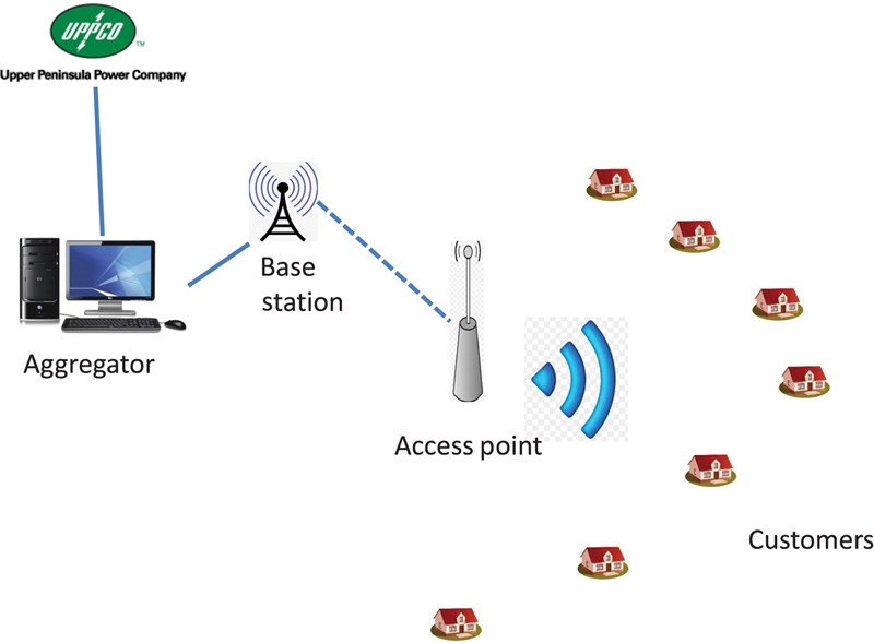
Figure 10.1 System Model
Despite the benefit it offers, the smart home system is vulnerable to cyberattacks. A hacker can launch cyberattacks on the basis of the connection and devices. Especially, the hacker can easily tamper a smart meter and manipulate the pricing information received by it, thus misleading the smart home scheduling of the customers. As is known, the modern smart meters are usually microcontroller based and installed with advanced embedded operation systems, which is vulnerable to virus and cyberattacks from the internet. For example, the smart meter of Texas Instruments is based on MSP430, which supports two-way communication such that the system can be remotely upgraded [8]. Remote upgrading makes the smart meter vulnerable to cyberattacks. In fact, multiple public media reports witness that various smart devices such as security camera, smart TV, smart doorlock, smart refrigerators, smart bulbs, and powered outlets became the targets of hackers [9–11].
In this book chapter, the impact of pricing cyberattacks to the smart home and the local community is analyzed. As is shown in our previous work [1], manipulating the guideline price can reduce the expense of the cyberattacker and increase the peak energy usage in the local power system. The detection techniques are then proposed to mitigate the impact of the cyberattacks and protect the smart home system. In order to identify the cyberattack, we predict the future guideline price from the historical data using support vector regression (SVR) and compare it with the one received by the smart meter. Since the electricity-pricing curve tends to be similar in short term, manipulation can be detected if the difference between the received guideline price and the predicted one are significantly different. Since the purpose of the detection technique is to limit the impact to local community and customers, the impact differences are defined to quantify the bill and the peak-to-average ratio (PAR) increase comparing the predicted guideline pricing curve and the received guideline pricing curve. When the impact differences are larger than some prespecified values, the cyberattack is reported to the utility to request for further check which is associated with human interaction.
This framework is used to detect the cyberattacks at each single time slot, which is defined as single event detection technique. The performance of the aforementioned single event detection technique is limited since it does not have a long-term view. The single event detection technique reports an alert if the impact differences are beyond the threshold. However, in many cases the impact differences are minor at each time slot while they can accumulate to be significant in long term. For example, suppose the threshold is set as 2%, which means that the cyberattack is reported if the received guideline electricity price can increase the average bill by 2%. However, if the hacker manipulates the electricity pricing to increase the bill by 1.9% each time slot, no cyberattack will be detected. However, the cumulative bill increase during the long term would be significant. The cumulative impact can be mitigated by lowering the thresholds. However, this could increase the labor cost for checking the smart meters significantly due to the fluctuation of the electricity-pricing curve. To tackle this problem, a long-term detection technique using partially observable Markov decision process (POMDP) is proposed in Ref. [1], which has the ingredients such as probabilistic state transition, reward expectation, and policy transfer graph to account for the cumulative cyberattack impact and its potential future impact. The general attacks targeting electricity pricing in smart grid have been studied in existing literature. The work in Ref. [12] proposes a jamming attack such that the attacker jams the communication network to block the updated electricity price. The work in Ref. [13] introduces false data injection attack to manipulate the real-time monitoring data to interfere the state estimation, which damages the power grid. Generally speaking, the cyberattacks in the smart home context includes the cyberattack on both input and output of smart meter as well as smart meter itself. Although the works in Refs. [12] and [13] present the cyberattacks targeting the input, the works in Refs. [14,15] studies energy theft, which is the cyberattack targeting the output such that the hackers attack their own smart meters to decrease the measurements of energy usage, thus saving the electricity bill of themselves. These works do not address smart home pricing cyberattacks since they do not consider the impact due to smart home scheduling. To mitigate the impacts of those attacks, defense techniques have been designed in literature. The work in Ref. [16] proposes a likelihood ratio-test-based algorithm to detect the malicious data attack on smart grid state estimation. The work in Ref. [17], proposes detection technique for jamming attack in time critical networks. The works in Refs. [18,19] study the countermeasure techniques against false data injection attack on the basis of sparse optimization and Kalman filter, respectively. Again, these works do not address the pricing cyberattacks in the smart home context.
In this chapter, the vulnerability of the smart home infrastructure will be assessed and the detection technologies against pricing cyberattacks will be discussed, which are based on machine learning techniques. In addition, the advanced control theoretical partially observable Markov decision process will be discussed. The salience of the algorithms will be demonstrated through simulation results.
2. Smart home system preliminaries
2.1. Smart home system model
A set of  customers supplied by a utility are considered in the system. Refer to Fig. 10.1. Each customer schedules the energy consumption during the next 24 h from the current moment, which is divided into H time slots and let
  . Each customer is equipped with a smart meter, which receives the electricity price from the utility and sends the measurement of real-time energy consumption to the aggregator. In the following, we will give an overview of the game model and solution of smart home scheduling, which have been developed in our previous work [20].
Each customer n ∈ N has a set of home appliances denoted by An. At each time slot h, the home appliance m ∈ An works under power level  , where Xm is the set of available power levels for home appliance m. In general, there are two categories of home appliances, namely, manually controlled home appliances and automatically controlled ones. The category of manually controlled home appliances consists of TV set, computer, refrigerator etc. The category of automatically controlled home appliances consists of washing machine, cloth dryer, dish washer, electric vehicle (EV) etc. It is worth noting that heating, ventilation, and air conditioning (HVAC) system could be classified into both categories. For example, the customer can adjust the working power level of the air conditioner manually according to the temperature in the room. However, there also exists situation that the customer needs the temperature to reach a certain level at a certain time point, in which the air conditioner works in the automatic mode. For each customer n, denote by Pn the set of manually controlled home appliances and denote by
  the set of automatically controlled home appliances. Thus,
  . For customer n, the total energy consumption of the manually controlled home appliances at time slot h is denoted by
  , one has
 (10.1)
where tm,h is the actual execution time of home appliance m at time slot h. At time slot h, the total energy consumption of automatically controlled home appliances is denoted by  , one has
 (10.2)
For each automatically controlled home appliance m ∈ Qn, the power level is chosen subject to the following constraints.
(1) The total energy consumption of the home appliance m is equal to the required total energy consumption Em. That is,
 (10.3)
(2) For a specified task, the home appliance m needs to be executed after the earliest start time αm and before the deadline βm such that
At each time slot h, the total energy load of the community is denoted by Lh, and thus
 (10.5)
As is mentioned before, there are two types of electricity prices in the smart home system, which are guideline electricity price and real-time electricity price, respectively. The guideline electricity price is provided to the customers to facilitate smart home scheduling, whereas the real-time electricity price is used in computing the bill.
In real-time pricing, at each time slot the monetary cost of energy consumption depends on the total energy load of the grid. In this paper, the quadratic cost function is used to compute the total monetary cost of all the customers, which is a popular pricing model used in literature [3,23]. The total monetary cost at time slot Ch is given as
where ah is the pricing parameter which models the relationship between energy consumption and monetary cost. At each time slot, the monetary cost is distributed to each customer according to the energy usage of the customer. For customer n, the monetary cost is denoted by Cn,h where
 (10.7)
2.2. Smart home scheduling
Given the aforementioned constraints, one can formulate a game where each customer n aims to minimize the individual monetary cost. Since the monetary cost of each customer n depends on the total energy load of the community including all the other customers, the scheduling of one customer has an impact on others. This naturally leads to a game. The monetary cost of each customer n can be divided into two parts. One has
where l–n,h is the community wide energy load excluding the energy consumption of customer n at time slot h and
 (10.9)
The game can be then formulated as follows [20].
Game model:
• Players: All the customers in the system.
• Payoff function: 
• Shared information: l–n,h.
• Problem formulation:
P1 
subject to 

In the game, each customer aims to minimize the total payment through scheduling the energy consumption of the automatically controlled home appliances. Nash equilibrium is achieved when no one can further reduce his/her own monetary cost without changing that of any other customer [24]. To solve this game, a decentralized technique proposed in our previous works [20,22] is used. This is an iterative algorithm. In each iteration, each customer solves the Problem P1 using the dynamic-programming-based algorithm while assuming the energy consumption of all the others, that is, l–n,h, is fixed [20]. After each iteration, each customer obtains the new energy consumption information from all others according to their updated scheduling solutions. With the updated energy consumption of each customer, l–n,h is updated and each customer uses dynamic programming to schedule their home appliances with the updated l–n,h. This process is iterated until convergence. For the scheduling of each customer, the home appliances are scheduled one after another. The method for the scheduling of single home appliance is described as follows [21].
The energy consumption of a home appliance is scheduled while assuming those of all others are fixed. Thus, if the power level of home appliance i at time slot xi,h is fixed, the total energy load can be directly calculated and the electricity bill can be derived. The dynamic-programming-based smart home scheduling algorithm aims to choose the power levels of a home appliance at each time slot to minimize the electricity bill. It proceeds one time slot after another from time slot 1. For time slot h, the accumulative energy consumption and corresponding electricity bill are computed for combination of power levels from time slot 1 to h. Among the combinations with the same accumulative energy consumption, only the one with the lowest monetary cost is maintained because it is the only one that could be a part of the final solution. An example is included as follows.
Consider a home appliance with three power levels and an operation period of four time slots. The electricity bill corresponding to each time slot and power level is given in Table 10.1. From time slot 1 to h, the combination of power levels is recorded as  . Starting from time slot 1, all power levels (1), (2), (3) are maintained because each of them has a unique accumulative energy consumption. Proceeding to time slot 2, the combination of power levels (1,2) and (2,1) have the same accumulative energy consumption, which is 3. However, the electricity bills are 3.5 and 3.2, respectively. Thus, only (2,1) is maintained since it has a lower electricity bill. Such a technique is applied to all other combinations of power levels. Thus, (1,1), (2,1), (3,1), (3,2), (3,3) are maintained from the original 9 combinations in the first two time slots. Combining them with all the available power levels at the third time slot, totally 15 combinations are generated for the total three time slots. Subsequently, (1,1,1), (2,1,1), (3,1,1), (3,1,2), (3,1,3), (3,2,3), and (3,3,3) are maintained. Proceeding to time slot 4 in the same way as before, totally 21 combinations are generated and (1,1,1,1), (2,1,1,1), (3,1,1,1), (3,1,1,2), (3,1,1,3), (2,1,2,3), (3,1,3,3), (2,3,3,3), and (3,3,3,3) are maintained. Suppose the given task requires an energy consumption of 5. The combination (3,1,1,1) is chosen since it has the same amount of total energy consumption with the requirement.
Table 10.1
Electricity Bill Corresponding to Each Power Level
| Monetary Cost ($) | Time Slot 1 | Time Slot 2 | Time Slot 3 | Time Slot 4 |
| Power level 1 | 1 | 1.2 | 1.5 | 1.1 |
| Power level 2 | 2 | 2.5 | 2.8 | 2.4 |
| Power level 3 | 3 | 3.8 | 4.1 | 3.6 |

The complete description of the smart home scheduling algorithm for multiple customers is presented in Algorithm 10.1. Three sets A, Cen, and Cmin are used to store the combinations of power levels, accumulative consumptions and electricity bills, respectively. The array current is a temporary variable to store the temporarily generated combination of power levels. In line 3, 4, and 5, the sets A, Cen, and Cmin are initialized as empty sets. In line 7, the electricity bills corresponding to each power level at each time slots are computed, which is similar to those in Table 10.2. In line 12, each power level is combined with the existing combination of power levels. The corresponding electricity bill C and accumulative energy consumption are calculated in line 13. From line 14 to line 20, the sets A, Cen, and Cmin are updated. The updating rule is as follows. If there is a combination of power levels with accumulative energy consumption Ce in A denoted by A(Ce), it is replaced by current if its corresponding monetary cost Cmin(Ce) is greater than C.Cmin(Ce) is also updated as C. If there is no combination of power levels with accumulative energy consumption Ce, Current is included in A as A(Ce). Ce and C are also included in Cen and Cmin as Cen(Ce) and Cmin(Ce), respectively. When all time slots have been proceeded, the combination of power levels with required accumulative energy consumption is returned in line 22.

Algorithm 10.1 The Scheduling Algorithm for Single Home Appliance
Table 10.2
Daily Energy Consumption and Regular Execution Duration of Automatically Controlled Home Appliances [20]
| Home Appliance | Daily Consumption | Execution Duration |
| Washing machine | 1.2–2 kWh | 1–3 h |
| Dish washer | 1.2–2 kWh | 1–3 h |
| Cloth dryer | 1.5–3 kWh | 1–3 h |
| EV | 9–12 kWh | 4–8 h |
| Air conditioner | 2–3 kWh | 2–3 h |
| Heater | 2–3 kWh | 2–3 h |
3. Pricing cyberattacks
Consider the communication infrastructure of the AMI in Fig. 10.1. First, the utility transmits the pricing information to a central computer in the local community (substation) through Internet. Second, such pricing information is broadcast to smart meters through Internet or WiFi network or a combination of them, depending on the communication infrastructure of the local community. For example, in a hierarchical infrastructure where a community consists of multiple subcommunities, pricing information is forwarded to each subcommunity through internet and is then broadcast inside the subcommunity through the WiFi network. In a WiFi network, there are some access points, which serve as the agents to receive the pricing information from the subcommunity and forward it to the smart meters inside the subcommunity.
The aforementioned popular infrastructure is vulnerable to at least three attacking strategies. First, one can directly hack the computer in the substation and modify the pricing information there. Subsequently, the pricing information forwarded to the whole community could be a faking one. Second, one can block an access point in the WiFi network using the jamming attack (ie, sending excessive requests to the access point), create a fake access point, and send the faking pricing information to the smart meters covered by the fake access point. Third, one can hack the smart meter and modify the pricing it receives. As is indicated by Ref. [25], “commercial smart devices including smart meters are often designed and manufactured utilizing off-the-shelf components and/or solutions. Therefore, security protection methods can only be applied at the application/network level and can hardly cover the hardware infrastructure. As a result, attackers can easily bypass firmware verification and install malicious OS kernel in the device to remotely control the smart device.” For example, an attacker could remotely manipulate the guideline pricing received at a smart meter without being realized. With the different difficulty levels in implementation, the cyberattacker can choose which one to use in practice.
3.1. Cyberattack for bill reduction
The first possible cyberattack is to fake the guideline pricing curve such that the utility bill of the cyberattacker can be reduced at the cost of bill increase of others in the community. Consider the following scenario. The guideline electricity price in the early morning such as 1:00 am to 8:00 am are usually not high due to limited amount of human activities. However, if a cyberattacker schedules a large load during this period, it could still be expensive. Therefore, if the cyberattacker fakes the guideline-pricing curve such that the electricity price during 1:00 am and 8:00 am is very high, then almost no customer in the community will schedule energy during this period. Subsequently, the cyberattacker can schedule his/her own large load there, resulting in the significant reduction of his/her own bill. Of course, such a reduction comes from the increase of the bill of other customers. The procedure for the cyberattack for bill reduction using pricing manipulation is as follows.
1. Determine the starting time ts and ending time te for the hacker to schedule his/her own energy load.
2. Manipulate the guideline electricity prices received at the target smart meters such that after manipulation the guideline prices are high from ts to te and low at other time slots.
3. Schedule his/her own energy load from ts to te. When the guideline electricity price is high from ts to te, the customers tend not to schedule the energy consumption there according to the smart home scheduling. This reduces the energy load during these time slots, and results in the decrease of the real-time electricity price there. Subsequently, the cyberattack could schedule the energy consumption from ts to te, and makes profit through saving his/her own bill at the cost of increasing the bill of other customers.
3.2. Cyberattack for forming the peak energy load
The second possible attack is to fake the guideline pricing curve such that a peak energy usage can be formed. Consider the following scenario. The guideline electricity price at 8:00 pm is usually expensive since the utility discourages the excessive energy usage during this period which is typically occupied with various human activities (eg, watching TV). If a cyberattacker creates a fake guideline pricing curve with very low price at this slot, significant amount of energy (eg, laundry load) will be accumulated there. This will form a peak in the energy usage, which could significantly impact the power system stability. The procedure for the cyberattack for forming a peak energy load using pricing manipulation is as follows.
1. Determine the starting time ts and ending time te of peak energy usage hours.
2. Manipulate the guideline electricity prices received at the target smart meters such that after manipulation the guideline prices are very low from ts to te.
3. A peak energy load will be formed from ts to te. If the guideline electricity price is very low from ts to te, the customers tend to schedule large energy load there due to smart home scheduling. This increases the energy load during this time period which could potentially form a peak in energy consumption.
4. Single event detection technology
The aforementioned two pricing cyberattacks need to significantly perturb the guideline pricing curves. The key to design the countermeasure is to identify the guideline pricing manipulation. Machine learning and statistical data analysis techniques would be natural choices since the typical guideline pricing curves should be similar to each other in a short term. In this work, we choose SVR since it tends to produce robust results [26].
After computing the predicted guideline price curve, one can compare it with the guideline pricing curve received at the smart meter. For comparison, one could compute the maximum difference between the two curves and signal an alert when it is larger than a threshold. To explore this idea, we define a set of thresholds, called the maximum tolerable impact differences. An example maximum tolerable impact differences could be up to 2% increase in PAR and up to 5% increase in bill. Given the predicted guideline pricing curve and the received guideline pricing curve, one can perform smart home scheduling simulations to compute the average bill and PAR for each of the two guideline pricing curves, and then compute the differences between them, called the actual impact differences. When the actual impact differences are larger than the maximum tolerable impact differences, a potential pricing attack is spotted and an alert signal will be sent to the utility to request for further check which could need some amount of human interaction. This work will develop such a framework.
Denote by vectors ap and a the predicted guideline electricity price and the received guideline electricity price, respectively. Denote by ∆B and ∆p the actual impact differences in bill and PAR, respectively. We also define two thresholds δB and δp which are the maximum tolerable impact differences in bill and PAR, respectively. If ∆B > δB or ∆P > δP, the smart meter treats the guideline electricity price as being manipulated due to cyberattacks. After computing the predicted guideline pricing curve ap, one can perform smart home scheduling simulations to compute the bill Bp and the PAR Pp. Similarly, one can compute the bill B and the PAR P through using the received guideline pricing curve. Subsequently, the bill increase rate is computed as  and the PAR increase is computed as
  . If ∆B > δB or ∆P > δP, an alert will be signaled.
and the PAR increase is computed as . If ∆B > δB or ∆P > δP, an alert will be signaled.5. Long-term detection technique
5.1. Motivation
As mentioned in Section 1, the single event detection would have low detection rate when the thresholds in impact differences are above those used by hackers. A straightforward solution is to lower the thresholds. However, this would result in significant false alarm due to the fluctuation of the electricity pricing. To tackle this limitation, we propose to integrate the single event detection with POMDP [27] such that the cyberattacks can still be identified while the false alarm is mitigated. The rational behind this idea is that due to the inherent long-term view provided by POMDP, even if one uses low thresholds in single event detection, the false alarm can be ameliorated through various POMDP ingredients such as the probabilistic state transition and reward expectation. Thus, the long-term detection technique can identify most of the possible cyberattacks without increasing the cost due to false alarms.
POMDP is an advanced control theoretic technique, which takes as input the real world states (eg, those corresponding to different cyberattack impacts) and generate actions (eg, fixing the hacked smart meters) as output. Since in reality one cannot directly obtain the state, POMDP approximately computes the states on the basis of the observations which are possibly with some uncertainties. For completeness, an overview of the POMDP technique proposed in Ref. [27] is presented as follows.
A typical POMDP problem is described as a tuple  [27,28]. The finite set S denotes the state space of the system. The finite set A denotes the action space containing all the available actions for the decision maker (eg, the local community in our problem). The transition from the state s to s′ while taking action a is defined using the corresponding transition probability
  , namely,
  . After taking action α at sate s, the decision maker receives a reward R(s′,a,s) if the next state is s′. The observation space of the system state is described as the finite set O. The mapping between states and observations is defined as
  , which is the conditional probability that the observation is o while action and state are a and s, respectively. The decision maker estimates the system state on the basis of observation and takes action based on it. Thus, state, observation and action are the three key components of POMDP.
The state space is given by the set  , where each state si ∈ S denotes that i smart meters are hacked. Thus, there are totally N+1 states for a community with N customers. The observation space is given by the set
  , in which oi ∈ O denotes that i smart meters are observed to be hacked. During the long run, the smart meters are continuously monitored and the utility or local community has the updated the observation of the system during each time slot.
Since the exact current state is not known, the decision maker estimates the number of hacked smart meters from the observation and judges if the cyberattack can introduce significant expected system loss. If it is the case, the decision maker needs to check and fix the hacked smart meters. Otherwise, it chooses to ignore the cyberattack since checking and repairing the smart meters are associated with labor cost. Thus, the decision maker has two available actions.
• action a0, monitor the system and ignore the cyberattacks;
• action a1, apply single event detection technique on each single smart meter to detect the hacked smart meters and fix them.
Note that the POMDP-based long-term detection technique contains observation as a key component, which is obtained by the single event detection technique. Each customer uses SVR to predict the guideline price and conduct smart home scheduling simulation with it. If the PAR or electricity bill corresponding to the received guideline price is sufficiently higher than that corresponding to the predicted guideline price, an alert signal is generated. The decision maker counts the total number of alerts and sets the observation according to it. For example, if there are n alerts, the observation is obtained as on.
One might wonder why integrating single event detection to POMDP would improve the detection rate while mitigating false alarm. This is essentially due to the inherent long-term view provided by POMDP. Even if low thresholds in single event detection induce false alarms, they can be ameliorated through various POMDP ingredients such as the probabilistic state transition and reward expectation, while the detection rate is significantly improved. The estimation of the state is defined as belief state b. The properties described in Ref. [27] for belief state are summarized as follows.
• The belief state  denotes the confidence level associated with each state. For example, the belief state for our problem can be
  , which means that the current system state is s0 with probability 0.8, s1 with probability 0.2 and other states with probability 0 according to the estimation. Each time when the new observation is obtained, the belief state is also updated according to the Bayesian rule as follows [27].
 (10.10)
where  is a normalizing factor. As is seen from Eq. (10.10), the new belief state depends on the last belief state, current observation as well as the last action. It also depends on state transition function and observation function, which are the underlying regulations of the POMDP.
• The state transition function T(s′, a, s) represents the transition of real world states, which are not completely observable. Thus, the belief state transition is modeled by [27]
 (10.11)
In Eq. (10.11),  is the same normalizing factor as in Eq. (10.10). When b, a and o are all given, b′ is deterministic and can be directly obtained from Eq. (10.10). Thus,
  is given as [27]
 (10.12)
• The reward function _ is defined on the basis of the belief state [27].
 (10.13)
which is the reward when the decision maker takes action a at belief state b.
• The decision maker will optimize the long-term expected reward. However, the future event imposes more uncertainty than the current. Thus, a discount factor is introduced to reduce the importance of future event in the optimization target and the expected reward is modified as discounted expected reward defined as  is the reward in step t. The optimal value of the discounted expected reward given the current belief state b is denoted as V*(b) such that [27]
is the reward in step t. The optimal value of the discounted expected reward given the current belief state b is denoted as V*(b) such that [27]P3  . Each time the decision maker intends to find the optimal action. He or she needs to consider both the reward in the present step and the discounted expected reward in the long future. During the long run, the decision maker receives the update of the observation each time slot, from which he/she estimates the belief state of the system. Given the belief state of the current system state, the decision maker obtains the optimal action by solving the optimization problem P3. The procedure for solving a POMDP problem is presented in the example given later.
. Each time the decision maker intends to find the optimal action. He or she needs to consider both the reward in the present step and the discounted expected reward in the long future. During the long run, the decision maker receives the update of the observation each time slot, from which he/she estimates the belief state of the system. Given the belief state of the current system state, the decision maker obtains the optimal action by solving the optimization problem P3. The procedure for solving a POMDP problem is presented in the example given later.5.2. Our POMDP-based detection
In our problem context, there are three types of transition functions, namely, state transition function, belief state transition function and observation transition function. We already show the belief state transition function in Eq. (10.11). In the formulation of the POMDP, state transition probability indicates the mapping between the system states at two adjacent time slots. Each action leads to the update of the system state. Action a0 does not reduce the number of hacked smart meters under the influence of the decision maker. The hacker can continue the cyberattack if it is not eliminated.
For example, it can hack more smart meters to increase the impact to the power system. Thus, the state transition function for action a0 is given as
where  is the probability that the hacker will hack i smart meters at next time slot if j smart meters are hacked at this moment.
In contrast to other works which use artificial model for state transition, this work uses model training to compute from the historical data. Although the real system state is not known in history, since action a0 does not change the system state, we can develop the state transition from the observation. In order to compute the state transition probability from the historical data, define an observation transition function as  , which is the probability that the observation transits from o to o′. Thus, the state transition can be derived from
 (10.15)
where  is the conditional probability that observation o is obtained after taking action a0 while the real state is s. .
 (10.16)
In Eq. (10.16), is the observation function defined in Eq. (10.18). Since the probability for each system state P(s) is not known, it is approximated by P(o).  is obtained from the historical data. For example, before action a0 is taken, o0 appears 10 times. After action a0, there are 5 times o0 transiting to o0, 3 times to o1 and 2 times to o2. Thus we have
  ,
,  and
and  . Derived from the historical data, the state transition function takes into consideration the long-term effect of cyberattacks. Taking action a1, the utility or local community applies the single event detection technique to each individual smart meter to determine whether it is hacked and the hacked smart meters will be fixed. The transition function for a1 is given as follows.
 (10.17)
The observation after taking a0 is given as
in which  is the probability that there are j smart meters hacked while i ones are observed to be hacked. If action a1 is taken, all hacked smart meters are checked and fixed by the single event detection technique, which is also the belief of the decision maker. Therefore, we have
 (10.19)
The cyberattacks induces loss to the power system. This is modeled by the reward functions. For the ease of optimization, the system loss is formulated as follows. Give two parameters  and
and  , where
  . If the total number of hacked smart meters , the system loss is
  . If
. If  , the system loss is
  . The action a1 needs human interaction and is associated with a labor cost. Without loss of generality, the labor cost can be separated into two parts. The on-site inspection cost CI and smart meter recovery cost CR. Once action a1 is taken, the on-site inspection cost is CI is no matter smart meter is fixed or not. Fixing each smart meter costs CR. Thus, the reward for a0 and a1 are given as follows.
 (10.20)
At each time slot, the long-term detection technique consists of two phases. (1) Monitor the system state and obtain the observation. (2) Solve the POMDP problem to compute the optimal policy and take corresponding action. According to Problem P3, the optimal action is based on the belief state, which depends on the current observation, last belief state as well as the action taken last step. Summarizing all the possible combinations of observations and corresponding policies, a policy transfer graph can be achieved, which is the output of POMDP. It shows the optimal action the decision maker can take given the current situation. The complete procedure of the proposed long-term detection technique is summarized in Fig. 10.2.
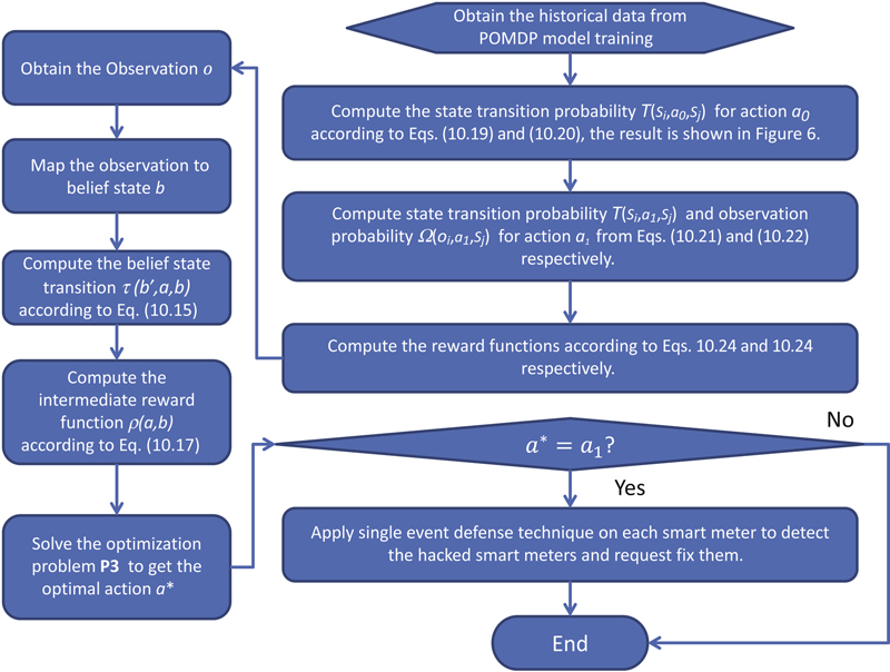
Figure 10.2 Algorithmic Flow of Our Proposed POMDP-Based Long-Term Detection Technique
6. Case study for long-term detection technique
Refer to Fig. 10.3. Consider a mini-community with two customers. A basic idea to define the states is that
• s0: no smart meter hacked
• s1: smart meter 1 is hacked
• s2: smart meter 2 is hacked
• s3: both smart meters are hacked.

Figure 10.3 State Definition of the Two-Smart Meter Example
There are totally two actions which are a0: ignore the cyberattacks and continue to monitor the smart meters and a1: check and repair the hacked smart meters. Each action can lead to the changing of the current state and corresponding to the new state, a new observation is obtained by the decision maker. In order to solve the POMDP problem, we need to consider the future transition of the states. This can be obtained by
• learning from historical data,
• calibrating the mapping from observation to state,
Using this method, the state transfer graph depending on each action is obtained as shown in Fig. 10.4. For example, starting from state s0, the transition probabilities are 0.5, 0.2, 0.2, and 0.1 to s0, s1, s2, and s3, respectively conditioned on a0.
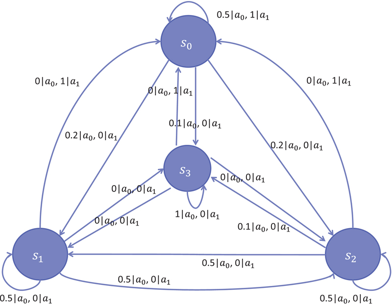
Figure 10.4 State Transfer Graph of the Two-Smart Meter Example
Since the detection method cannot be 100% accurate, the exact state is unknown to the decision maker. Thus, the decision maker depends on the estimation of the states to solve the POMDP problem. The estimation is defined as belief state b. For example, if there is no hacked smart meter, we have  , and b(s2) = 0. It is updated according to the Bayesian rule if a new observation is obtained according to Eq. (10.10). Note that checking and repairing the smart meters lead to labor costs. Similarly, a hacked smart meter can cause economical losses to the system. Thus, each action also corresponds to a reward. In order to solve the POMDP problem, the decision maker needs to consider the future expected reward and choose the action with the maximum one. Since the estimation of future event is less accurate than the current one, the reward of a future action is multiplied by a discount factor. Suppose the current belief state is
  , and b(s2) = 0, the procedure to compute the optimal action is depicted in Fig. 10.5. The maximum discounted expected rewards of each combination of belief state and action are denoted by
  , and R(s1,a1), respectively. The optimal action is a0 if
  . Otherwise, the optimal action is a1.
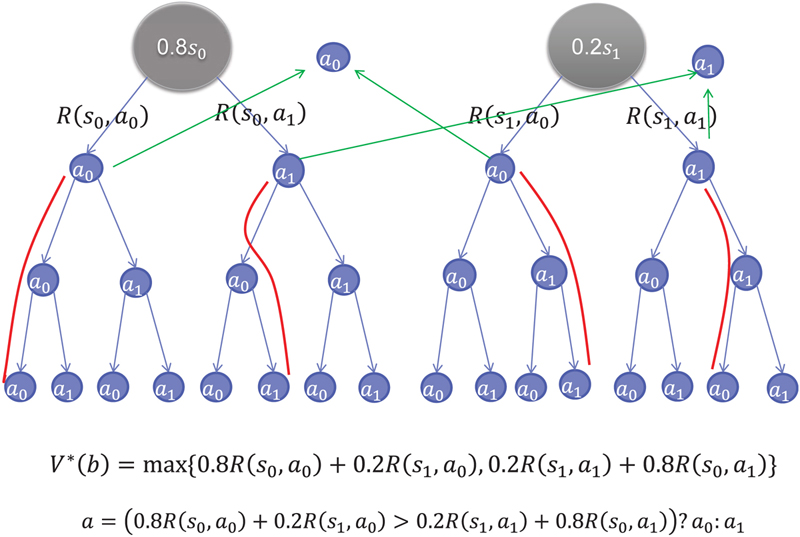
Figure 10.5 Computing Optimal Policy for the Two-Smart Meter Examples
As is discussed previously, the decision maker aims to choose the action with the maximum discounted expected reward. Assume the discount factor is 0.9 and we look three steps forward. At the current time slot t, there are two available actions. For each action taken at time slot t, there are two future available actions at time slot t+1. Thus, there are four available actions at time slot t+1 in total. Similarly, there are 8 available actions at time slot t+2. Computing the optimal expected discounted reward is actually computing the optimal path from the root to a leave of the tree. It can be solved using dynamic programming, which is a standard algorithm to solve this problem. , and R(s1,a1) are all calculated in this approach.
Using the standard solver of POMDP [29], a policy transfer graph can be computed as shown in Fig. 10.6. Initially, there is no hacked smart meter. Thus, we start from node e0 and take the corresponding action a0. If the obtained observation is o0, we remain taking action a0. If the obtained observation is o1, o2 or o3, we transfer to node e1 and take the corresponding action a1. After taking a1, o0 is the only possible observation. Thus, the system returns to node e0.
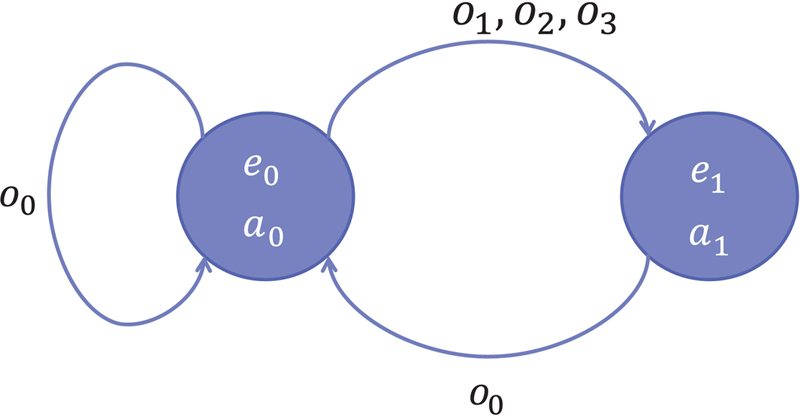
Figure 10.6 Policy Transfer Graph of the Two-Smart Meter Example
7. Simulation
The proposed algorithms are implemented using MATLAB and C programming language and simulations are conducted to analyze the impacts of smart home pricing cyberattacks and the performance of detection techniques. In the simulation setup, a community consisting of 500 customers is considered, and each customer is equipped with a smart meter connected with the AMI. For each customer, there are both manually controlled home appliances and automatically controlled home appliances. In our testcases, the average energy load due to manually controlled home appliances is shown in Fig. 10.7. The range for the daily energy consumption and regular execution duration of the automatically controlled home appliances are shown in Table 10.2, which is similar to our previous works [2,20]. The simulation duration is set to the next 24 h divided into hourly time slots. The quadratic pricing model is used. Therefore, y-axes in Fig. 10.8A, Fig. 10.9A, Fig. 10.10A, and Fig. 10.11A, B show the quadratic coefficients in pricing and one needs to multiple them by the energy load in the corresponding time slots to obtain unit price.
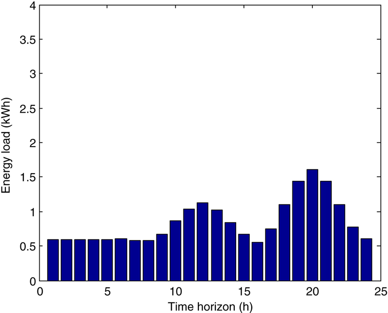
Figure 10.7 Average Energy Load by Manually Controlled Home Appliances (Background Energy Load)
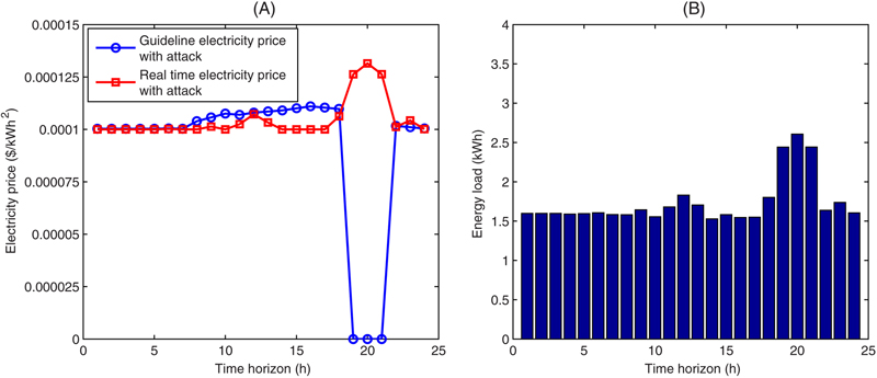
Figure 10.8 (A) Guideline electricity price and real-time electricity price without cyberattack. (B) Average energy load (PAR = 1.107) without cyberattack.

Figure 10.9 (A) Guideline electricity price and real-time electricity price with pricing cyberattack for bill reduction. (B) Average energy load (PAR = 1.358) with pricing cyberattack for bill reduction.
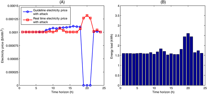
Figure 10.10 (A) Guideline electricity price and real-time electricity price with pricing cyberattack for forming peak energy. (B) Average energy load (PAR = 1.502) with pricing cyberattack for forming peak energy.

Figure 10.11 (A) Without cyberattack: for received guideline pricing, bill = $3.83, PAR = 1.170; and for predicted guideline pricing, bill = $3.82, PAR = 1.153, ∆B = –0.26% and ∆P = –1.45%. (B) With cyberattack: for received guideline pricing, bill = $3.83, PAR = 1.170; and for predicted guideline pricing, bill = $4.09, PAR = 1.203, ∆B = 6.79%, and ∆P = 2.82%.
7.1. Cyberattack for bill reduction
In this simulation, the smart home scheduling results with the unattacked guideline electricity price and the attacked guideline electricity price are compared. For the cyberattack, the hacker manipulates the guideline price and create a peak price from 1:00 am to 6:00 am and makes the rest flat. Refer to Fig. 10.8 for the results without attack and Fig. 10.9 for the results with attack, respectively. We make the following observations.
• From Fig. 10.8A, one sees that the guideline price well matches the real-time price, which is as expected.
• From Fig. 10.8B, one sees that the energy load is well distributed over the time horizon.
• In contrast, Fig. 10.9A shows that the guideline price and real-time price are significantly different. The reason is that when a smart home scheduler sees a high guideline price from 1:00 am to 6:00 am, it tends not to schedule the load there, which can be clearly seen from Fig. 10.9B. Note that there are still scheduled appliances during that time period due to (1) the background energy such as refrigerator and (2) the appliances which are required to be scheduled there due to starting time and ending time constraints. Due to the reduced energy usage from 1:00 am to 6:00 am, the real-time price at these time slots are lower than what it should be. Since the quadratic pricing model is used, the unit price is computed as the multiplication of quadratic coefficient (y axis) and the energy load. From 1:00 am to 6:00 am, the unit price is $0.0812 per kWh without cyberattack and is $0.0528 per kWh with cyberattack on average, which is a 34.3% reduction. Thus, if the hacker schedules his/her own load during this time period, a significant reduction in his/her own bill can be achieved.
This bill reduction of the hacker comes from the bill increases of other customers. Using the unattacked guideline electricity price, each customer pays $3.82 on average. However, using the attacked guideline price, the average bill increases to $4.12, which is 7.9% higher.
• As a byproduct, the cyberattack will also impact the energy load balancing. Comparing Figs. 10.8B and 10.9B, the PAR of the energy load from unattacked guideline electricity price is 1.107 while it becomes 1.358 with the attacked guideline electricity price.
7.2. Cyberattack for forming a peak energy load
In this simulation, the smart home scheduling results with the unattacked guideline electricity price and the attacked guideline electricity price are compared. For this cyberattack, the hacker manipulates the guideline price and creates a dip from 7:00 pm to 9:00 pm. Refer to Fig. 10.8 for the results without attack and Fig. 10.10 for the results with attack, respectively. We make the following observations.
• Fig. 10.10A shows that the guideline price and real-time price are significantly different. The reason is that when a smart home scheduler sees a low guideline price from 7:00 pm to 9:00 pm, it tends to schedule a large amount of load there, which can be clearly seen from Fig. 10.10B. The PAR of the energy load from unattacked guideline electricity price is 1.107 while it becomes 1.502 with the attacked guideline electricity price which is increased by 35.7%. This means that the cyberattacks can significantly unbalance the local energy load.
• Due to the peak energy usage from 7:00 pm to 9:00 pm, the real-time price at these time slots are higher than what it should be. From 7:00 pm to 9:00 pm, after converting quadratic pricing to unit price, one can obtain that the unit price without cyberattack is $0.160 per kWh and with cyberattack is $0.111 per kWh on average, which is a 43.9% increase. The average daily bill of each customer is $4.02, which is 5.24% more.
7.3. Single event detection technique
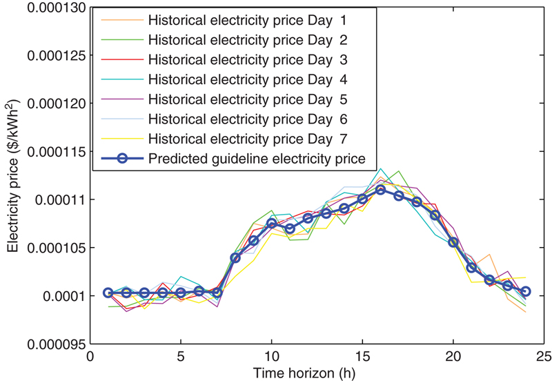
In this simulation, the performance of our proposed single event detection technique is evaluated. Given a set of the historical guideline electricity prices of last 7 days, a predicted guideline electricity price is computed using the SVR on these data. We have tested on various pricing cyberattacks. To present our simulation results, we assume that the hacker chooses to use a bill reduction cyberattack through increasing the guideline electricity price during some time slots. Refer to Fig. 10.11 for the simulation results. The maximum tolerable impact differences are set as δB = 5% for average bill increase and δp = 2% for PAR increase, respectively. We make the following observations.
• When there is no pricing cyberattack, Fig. 10.11A shows the received guideline electricity price and the predicted guideline electricity price. Comparing with the predicted electricity price, the average bill pay increase is −0.26%, smaller than δB and the PAR increase is −1.45%, smaller than δp. Thus, the received guideline electricity is regarded as normal.
• When there is pricing cyberattack, Fig. 10.11B shows the received guideline electricity price and the predicted guideline electricity price. Comparing with the predicted electricity price, the average bill increase is 6.79%, larger than δB and the PAR increase is 2.82%, larger than δp. In this case, the electricity pricing manipulation is detected.
7.4. Long-term detection technique
In the simulation, we consider five different communities consisting of 100, 200, 300, 400, and 500 customers, respectively, to evaluate the performance of the long-term detection technique. We analyze the performance of the proposed long-term detection technique using the policy transfer graph obtained by solving the POMDP problem. In order to show the advantage of our proposed method, the results are compared with those obtained from three other methods. In the first method, we repeatedly use the single event detection technique and recover the smart meters reported to be hacked, which is defined as the heuristic method. In the second method, a Bollinger-bands-based detection technique is deployed, which is a standard statistical data analysis method that is widely used in financial research, stock trading and time series analysis [30]. It computes the moving average and standard deviation of the historical guideline price during the last seven days. Subsequently, it computes an upper band and a lower band, which are K times the deviation above and below the moving average, respectively. They are known as Bollinger bands. Cyberattack is reported if the received guideline price is outside the bands. In the last method, no defense technique is deployed. The cyberattacks are randomly generated and the simulations are conducted for the time horizon of 48 h. The three methods are evaluated using observation accuracy, PAR increase, bill increase and labor cost for detecting hacks and fixing hacked smart meters. At each time slot, the observation accuracy is defined using the difference between the number of actually hacked smart meters and the number of smart meters reported to be hacked by each method. Precisely, the observation accuracy is defined as  if the observation is oi and the system state is sj (ie, j smart meters are actually hacked while i smart meters are reported to be hacked). The observation accuracies of the proposed method and the heuristic method for different testcases are shown in Figs. 10.12 and 10.13A, B, and Fig. 10.14, respectively. The results on bill increase, PAR increase and labor cost are shown in Table 10.3. For the 500-customer testcase, we make the following observations.
if the observation is oi and the system state is sj (ie, j smart meters are actually hacked while i smart meters are reported to be hacked). The observation accuracies of the proposed method and the heuristic method for different testcases are shown in Figs. 10.12 and 10.13A, B, and Fig. 10.14, respectively. The results on bill increase, PAR increase and labor cost are shown in Table 10.3. For the 500-customer testcase, we make the following observations.• Comparing with the results of no defense technique, the bill increase of and PAR increase are reduced by  and
and  , respectively.
and , respectively.
Figure 10.12 Observation Accuracy for 100-Customer and 200-Customer Testcases
(A) Observation accuracy for 100-customer testcase. (B) Observation accuracy for 200-customer testcase.
(A) Observation accuracy for 100-customer testcase. (B) Observation accuracy for 200-customer testcase.

Figure 10.13 Observation Accuracy for 300-Customer and 400-Customer Testcases
(A) Observation accuracy for 300-customer testcase. (B) Observation accuracy for 400-customer testcase.
(A) Observation accuracy for 300-customer testcase. (B) Observation accuracy for 400-customer testcase.
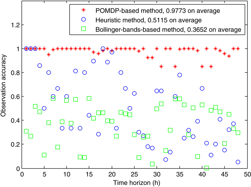
Figure 10.14 Observation Accuracy for 500-Customer Testcase
Table 10.3
Simulation Results of Detection Techniques
| Testcase | Parameter | No Detection | Bollinger Bands Method | Heuristic Method | POMDP-Based Method |
| 100-Customer | PAR increase | 32.1% | 4.03% | 6.85% | 2.87% |
| Normalized bill increase | 1 | 0.115 | 0.284 | 0.098 | |
| Normalized labor cost | — | 1.690 | 1 | 1.093 | |
| 200-Customer | PAR increase | 30.4% | 4.29% | 7.33% | 3.26% |
| Normalized bill increase | 1 | 0.118 | 0.289 | 0.102 | |
| Normalized labor cost | — | 1.601 | 1 | 1.074 | |
| 300-Customer | PAR increase | 31.8% | 4.47% | 7.82% | 3.24% |
| Normalized bill increase | 1 | 0.121 | 0.296 | 0.107 | |
| Normalized labor cost | — | 1.635 | 1 | 1.058 | |
| 400-Customer | PAR increase | 30.6% | 4.52% | 8.29% | 3.31% |
| Normalized bill increase | 1 | 0.125 | 0.309 | 0.112 | |
| Normalized labor cost | — | 1.669 | 1 | 1.087 | |
| 500-Customer | PAR increase | 31.3% | 4.57% | 8.40% | 3.42% |
| Normalized bill increase | 1 | 0.127 | 0.313 | 0.118 | |
| Normalized labor cost | — | 1.731 | 1 | 1.0816 |

• The Bollinger-bands-based detection technique has an accuracy of only 36.52%. Comparing with the Bollinger-bands-based detection technique, our proposed long-term technique can reduce the PAR increase by  and the normalized bill increase by
  , while still saving the normalized labor cost by
  . This is because the Bollinger-bands-based detection technique is a general statistical data analysis method without considering the specific problem nature of the smart home pricing cyberattacks.
and the normalized bill increase by , while still saving the normalized labor cost by . This is because the Bollinger-bands-based detection technique is a general statistical data analysis method without considering the specific problem nature of the smart home pricing cyberattacks.• Comparing with the heuristic method, our POMDP method has much better detection accuracy. It has the accuracy of 97.73% while heuristic method has the accuracy of 51.15%. In addition, our POMDP method can reduce the PAR and bill increase by  and
and  , respectively, at the expense of increasing the labor cost by only
  comparing with heuristic method since more smart meters need to be fixed. Again, the large improvements in detection accuracy, PAR and bill outweigh the small expense increase for our POMDP method. It demonstrates that our proposed long-term detection technique can more effectively detect the cyberattacks considering the cumulative effect, which cannot be handled by the single event detection technique. The results of the other testcases are shown in Fig. 10.12A, Fig. 10.12B, Fig. 10.13A, and Fig. 10.13B, respectively, which are similar with those 500-customer testcase.
and , respectively, at the expense of increasing the labor cost by only comparing with heuristic method since more smart meters need to be fixed. Again, the large improvements in detection accuracy, PAR and bill outweigh the small expense increase for our POMDP method. It demonstrates that our proposed long-term detection technique can more effectively detect the cyberattacks considering the cumulative effect, which cannot be handled by the single event detection technique. The results of the other testcases are shown in Fig. 10.12A, Fig. 10.12B, Fig. 10.13A, and Fig. 10.13B, respectively, which are similar with those 500-customer testcase.8. Conclusions
In this chapter, the smart home technique is presented, which enables the customers to schedule the energy consumption, thus avoiding using electricity energy during the peak pricing hours. This results in the reduction of electricity bill from the customer’s perspective and improvement of the energy-load balance from the utility’s perspective. Despite its effectiveness, this exposes the smart home system to malicious attacks. The impact of pricing cyberattacks is studied in the smart home context.
Two attacking strategies are developed, which can increase the electricity bill of the customers and the peak energy usage of the energy load, respectively. The detection techniques have been developed using partially observable Markov decision process to mitigate the impact of the cyberattacks. The simulation results demonstrate that the proposed long-term detection technique has the detection accuracy of more than 97% with the significant reduction in PAR and bill compared to a natural heuristic algorithm which repeatedly uses the single event detection technique.
..................Content has been hidden....................
You can't read the all page of ebook, please click here login for view all page.