Chapter 17

Smart restaurants: survey on customer demand and sales forecasting

A. Lasek*
N. Cercone*
J. Saunders
*    Department of Electrical Engineering and Computer Science, Lassonde School of Engineering, York University, Toronto, ON, Canada
    Fuseforward Solutions Group, Vancouver, BC, Canada

Abstract

Demand forecasting is one of the important inputs for a successful restaurant yield and revenue management system. Sales forecasting is crucial for an independent restaurant and for restaurant chains as well. In this chapter a comprehensive literature review and classification of restaurant sales and consumer demand techniques are presented. Sales prediction is very complex due to the impact of internal and external environment. However, a reliable sales forecasting methodology can improve the quality of business strategy. A range of methodologies and models for forecasting are given in the literature. These techniques are categorized here into seven categories, also including hybrid models. The methodology for different kinds of analytical methods is briefly described, the advantages and drawbacks are discussed, and relevant set of papers is selected. Conclusions and comments are also made on future research directions.

Keywords

restaurant sales forecasting
guest count prediction
revenue management
yield management

1. Introduction

Smart cities use digital technology in order to improve prosperity, reduce costs, reduce consumption of the resources, and enhance quality and efficiency of urban services. The aim of this chapter is to show an aspect important to cities—yield management with restaurants as an example.
Demand forecasting is one of the important inputs for a successful restaurant yield or revenue management (RM) system. Sales forecasting is crucial for an independent restaurant and for restaurant chains as well.
Nowadays, especially for big restaurant chains, a large number of time-ordered data are collected online and in real time, which results in massive amounts of data. Each time a customer order is placed, the transaction is automatically processed through the point of sale (POS) system and stored in a back-office database. Every POS system has the ability to track sales, cash, and inventory. And it also can track employee productivity, average sales per employee, what menu items are the most popular, and how quickly orders are served from time of input. Other possible reports include the number of customers served on an hourly and daily basis and the number of table turns. Restaurants with many locations can change menu items and prices with the POS system. It makes many restaurant chains collects massive datasets.
As mentioned in Ref. [1] from 1999 information technology eventually became so complicated that it can be integrated tool for decision making management and control of operations for restaurants. Furthermore, restaurant chains eventually grew large enough to support large investments that might be required. According to the authors, IT investments should be evaluated taking into account all aspects of restaurant management: production systems (including demand forecasting), planning (in both the kitchen and the dining room), process controls (including the management of meal times and production kitchen), and enterprise resource planning (enhanced back-office). Nowadays the most valuable are the data that could help to manage the three most important variables for the restaurants: food cost, labor cost, and demand forecast.
The sales transaction data collected by restaurant chains may be analyzed at the store level, the chain level, and the corporate level. For example, Cara Operations Limited—one of Canada’s largest owners of chain restaurants—owns 837 restaurants across the country under 10 brands including Swiss Chalet, Milestones, Kelsey’s, etc.
At the level of single store, exploring the large amounts of transaction data allows each restaurant to improve its operations management (eg, labor scheduling), product management (eg, Purchasing Management, product preparation scheduling), and supply chain management, and in consequence reducing restaurant operating costs and increasing quality of serving food (Fig. 17.1), whereas at the corporate level, extraction of relevant information across the restaurants can greatly facilitate corporate strategic planning (Fig. 17.2). Management can assess the impact of promotional activities on sales and brand recognition, assess business trends, conduct price elasticity analysis, and measure brand loyalty [2]. Thus, how to obtain an accurate and timely sales forecast is critical from many different perspectives.
image
Figure 17.1 Aims of Exploring the Sales Transaction Data at the Store Level
image
Figure 17.2 Aims of Exploring the Sales Transaction Data at the Corporate Level
Historically, restaurant managers have used a mental model or a simple rule using recent history to forecast guest counts. As mentioned in Ref. [3] forecasting of restaurant sales has been judgmental based and even in the 1990s this technique was most often used by the majority of the restaurant industry. Judgmental techniques consist of an intuitive forecast based on the manager’s experience. But restaurant sales forecasting is a complex task, because it is influenced by a large number of factors, which can be classified as time, weather conditions, economic factors, random cases, etc. This makes judgmental techniques inaccurate. A wide variety of models, varying in the complexity form, have been proposed for the improvement of restaurant forecasting accuracy.
Naïve forecasts are the simplest forecasting models, and provide a baseline, a benchmark against which more sophisticated models can be compared. Naïve method for time series data produces forecasts that are equal, for example, to the last observed value. Or if the time series is seasonal, more appropriate naïve approach may be applied when the prediction is equal to the value from last season (eg, last week, last month, last year, or the appropriate week 1 year ago) [4].
The state of menu-item demand forecasting was established in 1988 and can be found in Ref. [5]. The authors prepared a survey to assess the prediction techniques used by food service directors in a sample of American Dietetic Association Members with Management Responsibilities in Health Care Delivery System. The analysis of the replies showed that Naïve models were used by the majority of respondents. Only less than 25% were using mathematical models to forecast menu-item demand and Moving Average (MA) technique was the most popular mathematical model. But about 75% of the respondents indicated that learning and searching for a forecasting technique that can be used in the food service management is needed [5].
Limited empirical research has been carried out on restaurant sales predicting at the chain level. An investigation of the process of sales forecasting in corporate restaurants was conducted in 2006 and is presented in Ref. [6]. This qualitative study evaluates the sales forecasting process in the commercial restaurants. It consisted of interviewing 12 corporate restaurant forecasting managers responsible for the sales forecasting process for their companies. The results show that commercial restaurants are not enough advanced in forecasting techniques and the study provided recommendations for the companies to improve their sales forecasting processes.
Forecasting is a vast subject, covering a wide range of disciplines, including statistics, computer science, engineering, and economics. Over the years, a basic set of forecasting methods has been developed, but new improvements are still being added. Some of these prediction methods are based on rigorous mathematical and statistical basis, while others are largely heuristic in nature.
Perishability of food makes sales forecasting a unique problem in the restaurant, or generally speaking food service industry, because it relates to food purchased or wasted during production. Forecasting in the food industry is valuable in view of different aspects of the business. Food service managers have to predict sales to plan staff schedules and purchase food and supplies. Most of the meals are prepared right before service. In case of overprediction, when the demand is less than the forecast, there occurs a problem of leftover food and wasted resources, and in consequence it leads to increased food cost. In addition, overforecasting increases labor costs, because the extra handling of food requires additional use of employees. On the other hand, underforecasting leads to depletion of food before customer demand will be satisfied, thereby reducing food revenue and market share. Moreover, underforecasting causes insufficient number of staff and, consequently, customer dissatisfaction with service [7]. Thus accurate forecast is a definite goal of food managers, who aim to achieve a successful business.
Yet there does not exist any review of forecasting methods for the restaurant industry or any reports that describe the performance of various forecasting methods in restaurant RM applications. The aim of this chapter is to survey and classify restaurant sales forecasting techniques published over the past 20 years. Some of the content of this review was published as part of a conference paper [8].
The rest of this chapter is organized as follows. Section 2 contains basic information on yield management for restaurants and an overview of the role of forecasting for RM. Based on literature review we specified seven categories of restaurant forecasting techniques:
1. multiple regression;
2. Poisson regression;
3. exponential smoothing and Holt–Winters model;
4. autoregressive (AR), MA, and Box–Jenkins models;
5. neural networks;
6. Bayesian network;
7. hybrid methods.
They are arranged in roughly chronological order and discussed in Section 3. Section 3 is divided into eight subsections, one subsection for each category of restaurant forecasting techniques, and the eighth subsection describes application of Association Rule Mining for the restaurant industry. Every subsection provides a brief verbal and mathematical description of each technique and gives a literature review of a representative selection of publications in the given category. Section 4 presents a summary of all described methods and the discussion of advantages and disadvantages of each of the methods. Section 5 includes summarizing of our research and some remarks.

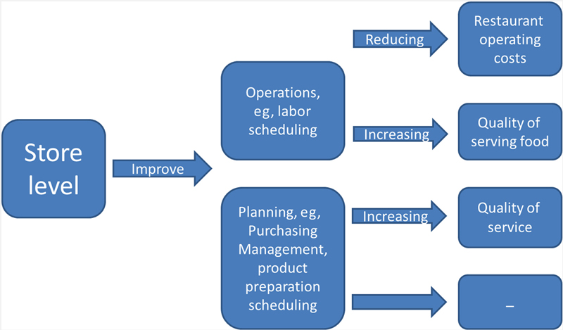
2. Revenue management

The first definition of RM was given by Smith et al. in 1992 as “selling the right inventory item to right customer at right time at right price” [9]. The determination of “right” entails both achieving the most revenue possible for the company and delivering the greatest utility to the customer [10]. Without this balance, the strategy of RM will in the long term discourage those customers who feel that the restaurant acts dishonestly.
A pioneer in RM was airline industry [11]. Other examples of industries in which RM is implemented nowadays are hotel industry, car rental companies, tour operators, cruise ship lines, transport companies, advertising (radio, TV broadcasters, and the most important nowadays: online advertising, eg, Google), energy transmission company, production, financial services and clothing retailers, restaurants, and others (Fig. 17.3).
image
Figure 17.3 Examples of Industries With Revenue Management
Now RM in the airline industry is highly developed professional practice based on a scientific basis. The core methodology of RM developed for use in the airline industry (and related industries, eg, hotels) over the past 25 years is briefly described in, for example, Ref. [12]. There are also given some insights into use of simulation in the RM. This airline success leads to the rapidly growing interest in using RM techniques in other industries. With every new application in the industry, there occur new challenges in modeling, forecasting, and optimization as well, so research in this area continues to grow. For example, in some of these industries customers have accepted dynamic pricing, while in restaurants definitely not (daily special is the one exception). Although the details of RM problems may significantly change from one sector to another, the emphasis is always placed on making better demand decisions—rather not manually, with guesswork and intuition, but with scientific models and technologies.
Restaurant sector is sufficiently similar to the hotels’ and airlines’ ones in the area of RM. A short comparison of restaurant and hotel RM can be found, for example, in Ref. [13]. However, the restaurants also have unique features that pose particular challenges, requiring operators to creatively develop appropriate RM strategies. Among the unique features of restaurants there are relative flexibility of capacities and flexible meal duration, and these are important topics to consider when implementing RM in restaurant. Unlike airlines and hotels, restaurants have a little more flexible capacity, for example, a restaurant may have outside patio for additional seating during days with a good weather. What is more, the total available number of seats per day in the restaurant is not set, since customers’ duration of meals are unpredictable [14]. However, restaurant can manage table turn rate.
In practice, RM means determining prices according to forecasted demand so that price-sensitive customers who are willing to purchase at off-peak times can do it at lower prices, while customers who want to buy at peak times (price-insensitive customers) will be able to do it [15]. For restaurant industry RM can be defined as selling the right seat to the right customer at the right price and for the right duration [16]. The goal for restaurant RM is to maximize revenue by manipulating price and meal duration. The price is quite obvious target for manipulation and many operators already offer price-related promotions to expand or shift peak period (eg, early bird specials, special menu promotions). More complex manipulation of price include setting price for a particular part of the day, day-of-week pricing, and price premiums or discounts for different types of party sizes, tables, and customers. Management of meal duration is a bit more complicated. Reduction of meal duration can be achieved by modifying the service process, changing the number of employees, or altering menu [16].
The RM strategy is the most effective when it is applied to operations that have the following attributes: relatively fixed capacity, demand that is time variable and predictable, perishable inventory, and the relevant costs and pricing structure [10]. All these attributes can be found in the restaurant industry.
The definition of capacity depends on the industry. Capacity is usually based on physical characteristics (eg, hotel capacity is usually measured by rooms, and airlines capacity is measured by seats), but in some cases it is also measured by time (eg, consulting companies), or working hours (eg, golf courses) [15]. Capacity of restaurants can be measured in seats, kitchen size, menu items, and number of employees. Kitchen capacity, the menu design, and members of staff capabilities are just as important as the number of seats in the restaurant. Capacity is usually determined in the short term, although many industries have a certain flexibility to be able to either reconfigure their capacity or add additional short-term opportunities. For example, airlines can reconfigure the seats or change the size of the plane, which is assigned to the route [15]. The number of places in the restaurant is generally fixed in the short term, although usually there is a possibility to add some number of tables or seats depending on reconfiguring the dining room, using outdoor seats at patio during nice weather, or adding patio heaters or shade to extend the range of conditions over which patios can be utilized. Adjusting the efficiency of a kitchen is usually more expensive, although output cuisine can often be improved by changing the menu or menu complexity or by increasing the level of employment. Despite all these possibilities for changes, restrictions in the kitchen and in the dining room can make the changes fruitless. Thus, restaurants’ capacity is basically constant [10].
The restaurant demand consists of people who make reservations and guests who walk in and all guests in total are a set from which managers can choose the most profitable mix of customers. One particular factor for restaurant operators is that they must take into account the length of time a party stays once it is seated. If the restaurant managers can accurately predict the duration of the meal, they can make better reservation decisions and give a better estimate of the waiting time for walk-in guests. Reservations are precious, because they give the company the possibility to sell and control their inventory early on. Moreover, companies that take reservations have the ability to accept or reject the reservation request, and they may use this possibility depending on the periods of high or low demand. Both of these types of demand can be managed, but they require different strategies. To forecast the demand and make a RM, the restaurant operator has to analyze the rate of bookings and walk-ins, guests’ desired times for dining, and probable meal duration. Tracking patterns of guests’ arrivals requires an effective reservation system [10].
Companies that use the RM have the perishable capacity that cannot be stored for later use, for example, a vacant seat in the airplane or unfilled cabin on a cruise cannot be recovered. For this reason, many industries consider offering discounts or promotions to be able to fill their unused capacity [15].
Restaurant’s inventory can be thought of as its supply of raw food or prepared meals. Instead, restaurant inventory should be considered as time, as the period during which a seat or a table is available. If the seat or the table is not occupied for a period of time, that part of the inventory perishes. Instead of counting table turns or income for a given part of the day, restaurateurs should measure revenue per available seat hour, commonly referred to as RevPASH. This is a measure defined by Klimes in Ref. [16], which captures the time factor involved in the restaurant seating. This is a consequent extension of the measurement commonly practiced in other industries that use RM, which focuses on the revenue per available inventory unit. For example, hotels measure revenue per available room-night (RevPAR) and airlines measure revenue per available seat-mile (RPSM).
As was mentioned before, industries that use RM, including restaurants, have appropriate costs and pricing structure. The combination of relatively high fixed costs and low variable costs gives them even more motivation for the fulfillment of their unused capacity, for example, restaurants must generate sufficient revenue to cover variable costs and offset at least some of the high fixed costs. And the relatively low variable costs give these industries some pricing flexibility and give them the opportunity to cut prices in periods of low demand [15]. However, the cost structure is quite different for restaurants compared to hotels and airlines. Variable cost (food and labor) in a restaurant is about 50%, which is much lower than in the mentioned industries.
Customer demand has two components: its timing and the duration of customer experience [15]. Customer demand will be different depending on the time of year, day of week, and time of day. For example, in a restaurant, it may be higher on weekends, or at specific times during periods of lunch or dinner. Time can be sold directly or indirectly. When companies sell time explicitly (eg, by the day as in the case of hotels), they are better able to control their capacity, because they know how long customers will be using the capacity, while companies that sell time indirectly (eg, restaurants) usually sell service experiences. An attempt to control customer duration is a very delicate issue due to the potential impact on customer’s experience and satisfaction. For example, in case of restaurant it has to reckon with the length of time a party stays once it is seated.
A RM system requires predictions of quantities such as customer demand, price sensitivity, and cancellation probabilities, and its performance depends vitally on the quality of these forecasts. But the most critical element in a strategy for restaurant RM is good prediction of future demand. Restaurant managers have always struggled with the question of how many guests will show up this day. Customer demand varies by the time of year, month, week, day, and the day part. Restaurant demand may be higher on weekends (especially on Fridays and Saturdays), during holidays, during summer months, or at particular periods such as lunch or dinner time. Restaurant operators want to be able to forecast time-related demand so that they can make effective pricing and table-allocation decisions [10].
From a practical point of view it is useful to predict demand (guest count) at different time intervals. They are listed in Table 17.1. Note that demand estimates made during the day can be very accurate but often local labor laws prohibit sending staff home without working a minimum number of hours, and it can be impractical to call in staff on short notice. Also, if the restaurant is overstaffed, it is expensive for the restaurant, and the staff is unhappy because they have to share the tips.

Table 17.1

Time Intervals in Which Restaurant Demand Should Be Predicted

No. Time Interval Range of the Interval
1 Month Next 12 months
2 Week Next 4–6 weeks
3 Day Next 7–10 days
4 Day part Next 1–3 days
Many RM systems in practice rely primarily on historical sales data to build forecasts. While this leads to highly efficient systems for data collection and automatic forecasting, relying solely on historical data has its weaknesses. For example, in media RM predictions for rating of new programs must be done, despite the fact that their ratings have often little relationship with the ratings observed for previous programs. Similarly, when the restaurant chain opens a store in a new city, there is often little or no historical data on which to base predictions. Moreover, even if the product remains constant, significant changes in the economy, competing technologies, or industry structure may cause the historical data not enough useful in predicting the future.
Thus, sales forecasting is the answer to the question how high will be sale under certain circumstances. The circumstances include the nature of sellers, buyers, and the market (eg, competitors). Sales prediction is very complex, precisely due to the impact of internal and external environment. However, a reliable sales forecasting can improve the quality of business strategy. Thus, important factors are historical sales data, promotions, economic variables, location type, or demographics of location. All variables that are useful in predicting demand and can be crucial in improving the accuracy of forecasts are listed in Table 17.2. A multicriteria decision-making method used to rank alternative restaurant locations is presented in Ref. [17]. In Ref. [18] important attributes for restaurant customers are presented, which can help in determination and prediction of customers’ intentions to return.

Table 17.2

Variables That Can Be Used as Predictors

No. External Variable Range or an Example of the Variable
1 Time Month, week, day of the week, hour
2 Weather Temperature, rainfall level, snowfall level, hour of sunshine
3 Holidays Public holidays, school holidays
4 Promotions Promotion/regular price
5 Events Sport games, local concerts, conferences, other events
6 Historical data Historical demand data, trend
7 Macroeconomic Indicators (useful for monthly or annual prediction) CPI, unemployment rate, population
8 Competitive issues Competitive promotions
9 Web Social media comments, social media rating stars
10 Location type Street/shopping mall
11 Demographics of location (useful for prediction by time of a day) The average age of customers

CPI, consumer price index.

Ref. [19] provides empirical evidence on the impact of online consumer reviews in the restaurant industry. The author investigated this issue with reviews from Yelp.com and restaurant data from the Washington State Department of Revenue. Yelp.com is the dominant source of consumer opinions in the restaurant industry. The researcher presented a few proposals concerning the impact of consumers’ opinion about the restaurant industry. First, a one-star increase in Yelp rating leads to an increase of 5–9% in revenue for independent restaurants, depending on the specification. This effect applies only to independent restaurants; ratings do not affect chain restaurants. Because chains already have relatively little uncertainty about quality, their demand does not respond to consumer reviews. Second, restaurants with chain affiliation have declined in market share as Yelp penetration has increased, which suggests that online consumer reviews substitute for more traditional forms of reputation. The reaction of consumers is larger when ratings contain more information. However, consumers also respond more strongly to information that is more visible, which suggests that the way information is given matters.
Ref. [20] brought an overview of work related to the Restaurant Revenue Management (RRM) that was made until 2010. The author notes that, despite the fact that history of the topic of increasing restaurant profitability dates back about 50 years, there are a surprising number of important and unanswered questions. These questions are not only those that might interest scientists but also those that may be relevant to the performance of individual restaurant, and the restaurant industry as a whole. And a part of these questions is related to the area of restaurant forecasting.
The RM application in restaurant industry is described in Ref. [21]. This is a case where the scientists worked with a local restaurant to test their ideas, make recommendations for improvement, and watch the results. This article describes how RM strategy was developed for the 100-seat casual restaurant in Ithaca, New York. Five tasks are listed for managers who want to develop an RRM program: (1) establish the baseline of performance, (2) understand the drivers of that performance, (3) develop a strategy for RM, (4) implement this strategy, and (5) monitor results of the strategy. An example from hotel industry was mentioned, where hotel RM system produced daily forecasts for the next 2–3 months and all forecasts were classified as hot, warm, or cold. Business periods of high demand were considered to be hot, low-demand periods were considered to be cold, and other times were considered to be worm. And hotel managers developed different strategies for each of the expected demand levels. Analogously the authors of the paper found that similar approach could be used in the restaurant industry. The restaurant required one set of policies for slow times and a completely different set for the busy times. During the hot periods managers should try to reduce the duration of meals and possibly raise the prices in the menu, for example, by eliminating discounts. During cold times, managers need to focus on increasing the number of clients and possibly increase average checks.
Maximizing productivity is extremely important for large and popular restaurants to increase their profits and remain competitive. The challenge of their floor managers is to decide when and where to seat each arriving guest. So, a tool that could help floor managers make better decisions would be very valuable to the restaurant. Authors of article in Ref. [22] claim that restaurants can increase their revenues by optimizing their nesting decisions, for example, when to save tables waiting for larger parties, even when there are smaller parties currently in the line. They developed mathematical programming models for RRM and showed that by saving tables in anticipation for larger parties, management can increase revenue, even when there are smaller parties waiting in the line. They created two classes of optimization models to maximize restaurant revenue, while controlling the average waiting time and the perception of fairness that may violate the first-come-first-serve rule. In the first class of models, the total programming, stochastic programming, and approximate dynamic programming methods were used in order to dynamically decide when to seat an incoming party in the restaurant that does not accept reservations. In the second class of presented models, researchers used the stochastic gradient algorithm to decide when, if at all, to accept a reservation. As shown by results using simulated data and those using real data from a restaurant, both of these models lead to significant improvements in revenues compared to using the first-come–first-serve policy.
In Ref. [23] authors provide an introduction to research in restaurant pricing. Restaurant operators set prices in a cost-based, demand-based, or competition-based way. As a part of a demand-based pricing, a restaurant aims to determine the right price for a menu item by understanding how price affects demand. Usually, there are three approaches that are used to estimate the impact of price on demand: estimation of customer willingness to pay, menu engineering, and price elasticity analysis.
Most companies have customer segments that are price sensitive and others that are not. Some clients may be willing to change the time of their use of service capacity in exchange for a lower price. On the other hand, some customers are less price sensitive and they are willing to pay a premium for the desired place at the desired time. Managers need to be able to identify different segments, and then adjust the price within a specified time to meet the needs for a given segment [15].
In 2013 the authors Kimes and Beard gave probably the most recent summary of the researches about RM in restaurant industry in a paper [24]. This article presented a framework for understanding the various aspects of RRM and to identify areas that need improvements and future research. Among other things, studies on how best to design the restaurant reservation system that take into account demand, meal duration, customer value, and table assignment would be very beneficial from scientists’ and managers’ point of view.

3. Literature review

3.1. Multiple regression

Multiple regression is a simple, yet powerful technique used for predicting the unknown value of a dependent variable Xt from the known value of two or more explanatory variables (predictors) V1, …, Vk. Multiple Regression uses least squares to predict the future and allow forecasters to experiment the effects of a different combination of the independent variables on the prediction. The equation for multiple regression is as follows:

Xt=0+1V1t++kVkt+ɛt

image
where ɛt is the error. Coefficients ∝0, …, ∝k can be estimated using least squares to minimize sum of errors [25].
For example, multiple regression models can be used in econometrics, where regression equation(s) model a causal relationship between the dependent variable (eg, restaurant sales) and external variables such as disposable income, the consumer price index (CPI), and unemployment rate. One of the advantages of econometric models created for predicting restaurant sales is that the researchers can logically formulate a cause-and-effect relationship between the exogenous variables and future sales or demand. Econometric models have however some drawbacks. Geurts and coworkers [26] noticed that the future values of the independent variables themselves have to be predicted, which can cause data in an econometric model to be inaccurate and the model to be weak in its ability to forecast. Also the relationship found between the dependent and independent variables may be pretended or their causal relationship can change over time, causing the need for constant update, or even a complete redesign of the model.
An example of using multiple regression is presented in Ref. [27]. The purpose of this study was to identify the most appropriate method of forecasting meal counts for an institutional food service facility. The forecasting methods included naïve models, MAs, exponential smoothing methods, Holt’s and Winters’ methods, and linear and multiple regressions. The result of this study showed that multiple regression was the most accurate forecasting method.
Also in Ref. [28] multiple regression model was used to demonstrate its potential for predicting future sales in the restaurant industry and its subsegments. Authors considered in this study the macroeconomic predictors such as percentile change in the CPI, in food away from home, in population, and in unemployment. They collected data from 1970 to 2011 from a variety of sources, including the National Restaurant Association (NRA), the United States Department of Agriculture (USDA), the Bureau of Labor Statistics, and the US Census Bureau. The model, trained and tested on aggregated data from the past 41 years, appears to have reasonable utility in terms of forecasting accuracy.
In Ref. [29] the author used several regressions and Box–Jenkins models to forecast weekly sales at a small campus restaurant. The result of testing indicates that a multiple regression model with two predictors, a dummy variable and sales lagged 1 week, was the best forecasting model considered.
Regression model was also used in a specific situation described in Ref. [30], where the restaurant was open and close during different times of the week or year.

3.2. Poisson regression

Restaurant guest count is an example of variable that takes on discrete values. When the dependent variable consists of count data, Poisson regression can be used. This method is one from a family of techniques known as the generalized linear model (GLM). The foundation for Poisson regression is the Poisson distribution error structure and the natural logarithm link function:

lnX=0+1V1++kVk

image
where X is the predicted guest count, V1, …, Vk are the specific values on the predictors, ln refers to the natural logarithm, 0 is the intercept, and i is the regression coefficient for the predictor Vi.
The method is used, for example, in Refs. [4,31]. In Ref. [32] authors noticed that Poisson Regression can be used to predict the number of customers being served at a restaurant during a certain time period.

3.3. Box–Jenkins models (ARIMA)

Time series models are different from Multiple and Poisson Regression models in that they do not contain cause–effect relationship. They use mathematical equation(s) to find time patterns in series of historical data. These equations are then used to project into the future the historical time patterns in the data. There are three types of time series patterns: trend, seasonal, and cyclic. A trend pattern exists when there is a long-term increase or decrease in the series. The trend can be linear, exponential, or different one and can change direction during time. Seasonality exists when data is influenced by seasonal factors, such as a day of the week, a month, and one-quarter of the year. A seasonal pattern exists of a fixed known period. And a cyclic pattern occurs when data rise and fall, but this does not happen within the fixed time and the duration of these fluctuations is usually at least 2 years [33].
The AR model specifies that the output variable depends linearly on its own previous values. The notation AR(p) refers to an AR model of order p. The AR(p) model for time series Xt is defined as follows:

Xt=c+i=1pϕiXti+ɛt

image
where ϕ1, …, ϕp are the parameters of the model, c is a constant, and ɛt is white noise. ɛt are typically assumed to be independent and identically distributed (IID) random variables sampled from a normal distribution with zero mean: ɛt ∼ N(0, σ2), where σ2 is the variance [10].
Another common approach in time series analysis is a MA model. The notation MA(q) indicates the MA model of order q:

Xt=μ+ɛt+θ1ɛt1++θqɛtq

image
where μ is the mean of the series, θ1, …, θq are the parameters of the model, and ɛt−1, …, ɛtq are white noise error terms [10].
In other words, a MA model is a linear regression of the current value of the series of the data against current and previous, unobserved white noise error terms, or random shocks. These random shocks at each point are assumed to be mutually independent and to come from the same, usually a normal distribution.
MA method is very simple, based on the idea that the most recent observations serve as better predictors for the future demand than do older data. Therefore, instead of having the forecast as the average of all data, a window with an average of only q previous observations is used.
MA reacts faster to the underlying shifts in the demand if q is small, but small span results in a forecast more sensitive to the noise in the data.
If the date shows up or down trend, the MA is systematically under projections or above forecast. To handle such cases, improvements such as a double or triple MA have been developed, but for this kind of data exponential smoothing methods are usually preferred, described in the next section.
AR and MA models were used to make a prediction for many different time series data. One of the examples is presented in Ref. [34], which is the first research looking into the casino buffet restaurants. Authors examined in this study eight simple forecasting models. The results suggest that the most accurate model with the smallest Mean Absolute Percentage Error (MAPE) and root mean square percentage error (RMSPE) was a double MA.
Another tool created for understanding and predicting future values in time series data is model ARMA(p; q), which is a combination of an AR part with order p and a MA part with order q. The general autoregressive moving average (ARMA) model was described in 1951 in the thesis of Whittle [35]. Given a time series of data Xt, the ARMA model is given by the following formula:

Xt=c+ɛt+i=1pϕiXti+i=1qθiɛti

image
where the terms in the equation have the same meaning as earlier.
An autoregressive integrated moving average (ARIMA) model is a generalization of an ARMA model. ARIMA models (Box–Jenkins models) are applied in some cases where data show evidence of nonstationarity (stationary process is a stochastic process whose joint probability distribution does not change over time and consequently parameters, eg, the mean and variance, do not change over time) [36].
Most of real-time series data turns out to be nonstationary. In such cases, the stationary time series models may not fit the data well and can produce poor prognosis. Techniques for dealing with nonstationary data try to make such data stationary by applying suitable transformations, so that stationary time series models can be used to analyze the transformed data. The resulting stationary predictions are then converted back to their original nonstationary form. One of such techniques is the differentiation of successive points in the time series. An autoregressive integrated moving-average process, ARIMA(p, d, q), is one whose dth differenced series is an ARMA(p, q) process.
Interesting case of big data mining project for one of the world’s largest multibrand fast-food restaurant chains with more than 30,000 stores worldwide is illustrated in Ref. [2]. Time series data mining is discussed at both the store level and the corporate level. To analyze and forecast large number of data researchers used Box–Jenkins seasonal ARIMA models. Also an automatic outlier detection and adjustment procedure was used for both model estimation and prediction.
A system designed to generate statistical predictions on menu-item demand in hospitals with intervals of 1–28 days prior to patient meal service is described in Ref. [37]. Authors used 18 weeks of supper data for analysis of menu-item preferences and to evaluate the performance of the forecasting system. There were three interdependent levels in the system: (1) Forecasting patient census, (2) predicting diet category census, and (3) forecasting menu-item demand. To assess the effectiveness of mathematical forecasting system and manual techniques a cost function was used. The costs of menu-item prediction errors resulting from the use of exponential smoothing method and Box–Jenkins model were about 40% less than the costs associated with manual system.
A paper considering the unique seasonal pattern in university dining environments is given in Ref. [7]. This study determines the degree of improvement in accuracy of each tested forecasting model in situation when the data are seasonally adjusted. Researchers compare the seasonally adjusted data and raw data and verify if seasonally adjusted data improves the accuracy. The data for this study is collected at a dining facility at a Southern university during two consecutive spring semesters. The customer count data of the 2000 spring semester was used as a base for forecasting guest counts in the 2001 spring semester. The data includes guest counts for dinner meals from Monday to Saturday, since the dining facility is closed on Sundays. Researchers selected six different forecasting methods including naïve model, MA method, Simple Exponential Smoothing, Holt’s Method, Winters’ Method, and Linear Regression. More sophisticated forecasting techniques, such as Box–Jenkins or neural networks, were not tested here. The accuracy of these models was assessed by Mean Squared Error (MSE), Mean Percentage Error (MPE), and MAPE. The results show that Winters’ method outperforms the other five methods when raw data is used. It turned out that seasonally adjusted data is much more effective in forecasting customer counts and significantly improve accuracy in most of used methods. All the other five mathematical forecasting methods outperform the naïve model when using seasonally adjusted data. And the MA method is the most accurate method of forecasting when seasonally adjusted data is used.
Overall, the main result of this study indicates that the use of seasonally adjusted data is critical for better forecasting accuracy in case of the university dining operations, where seasonal pattern certainly occurs. Thus the researchers strongly recommend employing the MA model with seasonally adjusted data to predict the number of customers in this kind of places.
Note, however, that the prediction of abnormal, extremely high or low demands is not considered in this study. In real situation, forecasting may be more complicated due to unexpected variables such as special events or unusual weather. Thus, the authors recommend for food service managers to employ techniques such as MA with the judgments from their own experience to get better forecasting results under their unique environment.

3.4. Exponential smoothing and Holt–Winters models

Exponential smoothing, proposed in the late 1950s, is another technique that can be applied to time series data to make forecasts. Whereas in the simple MA the past observations are weighted equally, exponential smoothing uses exponentially decreasing weights over time. The more recent the observation, the higher is the associated weight. For the sequence of observations {xt} beginning at time t = 0, the simplest form of the exponential smoothing algorithm is given by the following formula:

s0=x0

image

st=xt+(1)st1,t>0

image
where {st} is the estimation of what the next value of x will be, is the smoothing factor, and 0 <  < 1.
Triple exponential smoothing (suggested in 1960 by Holt’s student, Peter Winters) takes into account seasonal changes and trends. As we mentioned in the previous section, seasonality is a pattern in time series data that repeats itself every L period. There are two types of seasonality: multiplicative and additive in nature.
For time series data {xt}, beginning at time t = 0 with a cycle of seasonal change of length L, triple exponential smoothing is given by the following formulas:

Ft+m=(st+mbt)ctL+1+(m1)modL

image

s0=x0

image

st=xtctL+(1)(st1+bt1)

image

bt=β(stst1)+(1β)bt1

image

ct=γxtst+(1γ)ctL

image
where Ft+m is an estimate of the value of x at time t + m (m > 0), is the data smoothing factor, β is the trend smoothing factor, γ is the seasonal change smoothing factor, 0 < , β, γ < 1, {st} represents the smoothed value of the constant part (level) for time t, {bt} is the estimation of the linear trend for period t, and {ct} represents the sequence of seasonal factors.
Exponential smoothing was one of the most common and simple methods for food and beverage sales forecasting (eg, Refs. [38,39]).
The results of the study [3] show that for the actual sales in the restaurant, which is independently owned and located in a medium-sized university town, Box–Jenkins and exponential smoothing models performed as well as or better than an econometric model. Authors as an initial database used monthly observations of sales from 6 years from this restaurant. And they tested model on the next 7 months of data. Since time series models are usually more economical in terms of time and skill levels of the users, the results of this study are important for forecasting in the restaurant industry. Results of this paper suggest that for a restaurant manager with limited resources, an exponential smoothing model could usually give a very satisfactory forecast of sales. Forecast accuracy can be improved by using a Box–Jenkins model; however, this model is more complex.
Another study that compares different forecasting models to predict the meal participation at university residential dining facilities is presented in Ref. [40]. Authors used data collected from two dining rooms over 15 weeks to test naïve forecasting techniques, three different versions of MA, and simple exponential smoothing. The analysis of these prognostic models using Mean Absolute Deviations (MADs), MSEs, and MAPEs indicated that all the simple mathematical forecasting techniques provided better forecasts than naïve methods and MA methods gave the best results.
Another assessment of which forecasting model would most accurately predict meal demand is presented in Ref. [41]. The uniqueness of this study lies in the fact that the data do not relate to ordinary restaurant, but to congregate lunch programs located throughout the United States, designed for serving older adults. But lunch meal demand forecasting in this program has much in common with forecasting demand for restaurants. Food service managers in these programs are responsible for operational expenditure. Funds for that are made available to local meal providers as reimbursements based on meals served, in contrast to meals produced; thus the ability to accurately predict demand meal can become critical in an effort to maintain fiscal responsibility. Accurate forecasts allow food service managers to purchase adequate amounts of food and supplies, produce the right amount of meals, and properly plan a schedule for staff. Overproduction can lead to food waste and excessive costs, and on the other hand underproduction may create shortages that will affect customer satisfaction. Forecasting techniques, including naïve, three versions of MA, and simple exponential smoothing, are applied to data collected within 4 months from seven locations in large urban agglomeration. The author used MADs and MSEs to analyze all these methods. The results of the evaluation indicated that for all locations simple mathematical forecasting techniques provided better meal demand prediction than did the naïve method. In four of the seven sites, exponential smoothing outperformed the other methods, while in other places, MA models provided the best forecasts.
The extension of this paper can be found in Ref. [42]. This time data from eight different congregate meal sites in the Southern California area were used over the 6-month period. All sites utilized a nonselect 6-week cycle menu. As in the previous study the simple mathematical forecasting techniques provided a better prediction of meal demand than did the naïve method in all cases. The results of this study indicate that exponential smoothing outperformed the other prediction methods in all locations. The second aim of this paper was to answer the following research question: Could the accuracy of the forecast be improved when the historical customer count information will be obtained from the same day of the menu cycle instead of from the same day of the week? The results of this paper indicate that even though the lunch sites studied used a cycle menu, the effectiveness of the prediction method was not significantly improved when the same day of the menu cycle was used as the source of the historical data, as opposed to the same day of the week.
The aim of study [43] was to develop, test, and evaluate mathematical forecasting using entree demand data collected from a university dining hall food service. The used time series models are applicable to all types of food and beverage operations, because the used data contained typical gastronomy production variable: menu changes. Researchers employed naïve methods (used as the base case), simple MA, and simple exponential smoothing. They modeled both the total number of guests during the meal period and entrees on the menu (entree combinations). Once the guest count data were used, the forecast was then multiplied by a preferences statistic, which was calculated for each entree to forecast the percent of this entree that would be chosen when the entree combination was offered. Results of this study are consistent with other researches related to food service forecasting. The time series models outperformed the Naïve Model. The simple MA model gave smaller but more numerous forecast errors, whereas simple exponential smoothing did the reverse.

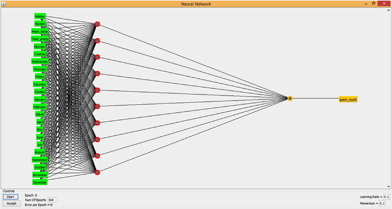
3.5. Artificial neural networks

All the forecasting methods we have discussed in previous subsections have the same strategy: make a functional assumption for the relationship between the observed data and various factors and then estimate the parameters of this function using historical data. In contrast, neural network methods and other machine learning algorithms use interactions in a network architecture to automatically estimate the underlying unknown function that best describes the demand process. Artificial Neural Networks (ANNs) are a class of models inspired by biological neural networks and studies of the human nerve system, in particular the brain. The methods are based on approaches that mimic the way the human brain learns from experience and are used to estimate or approximate functions that can depend on a large number of inputs and are generally unknown. In theory, with the suitably constructed architecture and with the properly carried out training procedure, neural networks are able to approximate any nonlinear function after a sufficient degree of learning.
ANNs are systems of connected neurons, where the connections have numeric weights that can be tuned based on experience from historical data, which causes that neural networks are adaptive to inputs and capable of learning.
ANNs are used for sales forecasting due to the promising results in the areas of control and pattern recognition. In Fig. 17.4 there is an example of neural network architecture for guest count prediction.
image
Figure 17.4 Example of Neural Network Architecture for Guest Count Prediction
In feedforward networks (or perceptrons)—the most important class of neural networks used for forecasting – the nodes of the network are arranged in succeeding layers, and the arcs are directed from one layer to the next, left to right as shown in Fig. 17.4. Training data is “fed” to the first (the input layer), and the forecast is “read” from the last (the output layer). Usually, in demand forecasting applications, each node in the input layer corresponds to the explanatory, and each node in the output layer corresponds to a single explanatory variable, for example, guest count. There are a number of hidden layers in between.
A set of training data is used to calibrate the weights and the value of the threshold functions. When these parameters are defined, the network can be used for forecasting. Thus, the three main steps are defining the network, training, and forecasting. There exist many procedures to automatically prune or grow the network topology on the basis of the observed data and network’s predictive performance, and many ways of improving training of neural networks, particularly in terms of speeding up the learning time or avoiding overfitting.
Ref. [44] compares ANNs and traditional methods including Winters’ exponential smoothing, Box–Jenkins ARIMA model, and multivariate regression. The results indicate that generally ANNs are more successful compared to the more traditional statistical methods. Analysis of experiments shows that the neural network model is able to capture the trend and seasonal patterns, as well as the interactions between them. Despite many positive features of ANNs, constructing a good network for a given project is a quite difficult task. It consists of choosing an appropriate architecture (the number of hidden layers, the number of nodes in each layer, the connections between nodes), selecting the transfer functions of the middle and output nodes, designing a training algorithm, selecting initial weights, and defining the stopping rule.
In the study in Ref. [45] authors combined an ANN and a genetic algorithm to design and develop a sales forecasting model. They collected historical sales data from a small restaurant in Taipei City and used them as the output for the forecasted results while associated factors including seasonal impact, impact of holidays, number of local activities, number of sales promotions, advertising budget, and advertising volume were chosen as input data. All the training and test data were preprocessed in such a way that the data were mapped between [1, −1]. And at the end an inverse transformation was performed on the results of prediction in order to restore the actual value of the forecasted sales. First, this approach applies the ANN to select the relevant parameters of the current sales condition as the input data. Then it uses a genetic algorithm to optimize the default weights and thresholds of the ANN. Researchers used empirical analysis to examine the effectiveness of the model. The results indicate that this is a scientifically practical and effective sales forecasting method that can achieve rapid and accurate prediction.
Fuzzy neural network with initial weights generated by genetic algorithm can be found, for example, in Ref. [46]. This study first proposes a genetic algorithm initiated fuzzy neural network that is able to learn the fuzzy IF–THEN rules for promotion provided by marketing specialists. This network can both learn fuzzy IF–THEN rules and incorporate fuzzy weights. The main reason for proposing this method is that the effect of promotion on sales is always very vague or fuzzy. The results from the fuzzy neural network are further integrated with the forecast from ANN using the time series data and the length of promotion from another ANN. In addition, this study also aims to develop an intelligent sales forecasting system based on the aforementioned concepts. Forecasting future demand is central to the operation of the convenience store companies, and the reliable prediction of sales can be a great benefit in improving the quality of a business strategy as well as decreasing cost, which means increased profit. Managers need sales forecasts as essential input to many decision activities.

3.6. Bayesian network model

Ref. [47] proposes a service demand forecasting method that uses a customer classification model to consider various customer behaviors. A decision support system based on this method was introduced in restaurant stores. Authors automatically generated categories of customers and items based on purchase patterns identified in data from 8 million purchases at a Japanese restaurant chain. The data was collected from 5 years from 48 stores. Researchers produced a Bayesian network model including the customer and item categories, conditions of purchases, and the properties and demographic information of customers. Based on that network structure, they could systematically identify useful knowledge and predict customers’ behavior. Details of this demand forecasting technique are given in Ref. [48].

3.7. Hybrid models

In the literature a hybrid approach to sales forecasting for restaurants is also proposed. The motivation of the hybrid model comes from the following prospects. It is often difficult in practice to determine whether one specific method is more effective in prediction then others. Thus, it is difficult for researchers to select the appropriate forecasting model for their unique situations. Usually, different approaches are tested and the one with the most accurate result is chosen. However, the final selected model is not always the best to use in the future. The problem of model selection can be facilitated by using combined methods [49].
Furthermore, it may not even be necessary to determine which method gives the best forecast: a linear combination of the predictions from two different models, with a properly chosen set of weights, may be constantly superior to any one of the component methods. This idea was proposed in the article in Ref. [50], and then investigated by other forecasting researchers. The intuition behind this result is that if the errors produced by two methods of prediction are negatively correlated, then combining them will reduce the overall forecast error.
Researchers use hybrid model in many different areas of forecasting. As an example of a hybrid system with excellent performance the model of daily product sales in a supermarket proposed in Ref. [51] can be shown. Authors combined ARIMA models and neural networks to a sequential hybrid forecasting system, where output from an ARIMA-type model is used as input for a neural network.
In Ref. [52] a research is presented not directly from the restaurant industry, but from a similar area of convenience stores, which provide multiple services, including daily fresh foods. Forecasting future demand is crucial for the functioning of such convenience store industry and reliable sales forecasts can be very beneficial in improving the quality of business strategy, as well as increasing profits by reducing costs. Sales forecasts are needed as an important contribution in various fields such as marketing, production, and sales. Here freshness and fast speed of turnover are important factors. Each store needs to have fresh food sales predicted accurately in order to maintain the high quality of sold products. In this study, an improved hybrid sales forecasting model of fresh foods, called Enhanced Cluster and Forecast Model, has been successfully developed. The model combines self-organizing map neural networks and radial basis function neural network. The model is evaluated for a 6-month sales dataset of daily fresh foods at a chain of 75 convenience stores distributed throughout Taiwan. According to the authors’ knowledge traditional convenience stores managers do not use a model approach for forecasting, or some of them use a fuzzy neural model. The proposed hybrid model not only is more efficient but also makes the model easier to build with greater accuracy. The proposed sales forecasting model is suitable for forecasting system in the real world.
For restaurant industry a hybrid methodology that takes advantage of the unique strength of ARIMA and ANN models in linear and nonlinear modeling and combines these two methods is proposed in Ref. [49]. In the real world time series data are rarely pure linear or nonlinear. They often contain both linear and nonlinear patterns. In this case, neither ARIMA nor ANNs may be suitable for modeling and forecasting time series. Hence, by combining ARIMA with ANN models, researchers can model data more accurately. Experimental results on sets with real data indicate that the combined model can be an effective way to improve accuracy of predictions achieved by each of the models used separately.

3.8. Association rules (market basket analysis)

In this subsection we want to mention an additional method that can help in restaurant forecasting. In Ref. [53] the problem of mining association rules and related time intervals is studied, where an association rule holds in either all or some of the intervals. As an example association rules in a given database of restaurant transactions are considered.
In Ref. [54] authors apply a simplified version of market basket analysis (MBA) rules to explore menu-item assortments, which are defined as the sets of most frequently ordered menu-item pairs of an entre and side dishes.
In some cases, MBA does not provide useful information if data item is the name of goods. In Ref. [55] authors propose a new MBA method that integrates words segmentation technology and association rule mining technology. Characteristics of items can be generated automatically before mining association rules by using word segmentation technology. This method has been applied to a restaurant equipped with electronic ordering system to give recommendations to customers, where the experiments were done. The experiment results show that the method is efficient and valid.

4. Discussion of methods and data mining algorithms

The summary of all approaches is presented in Table 17.3.

Table 17.3

Summary of Sales/Demand Forecasting Methods

Method Description Examples of Papers
Multiple Regression Multiple Regression uses least squares to predict the unknown value of a dependent variable from the known value of two or more explanatory variables (predictors) [2630,34]
Poisson Regression Poisson regression uses the Poisson distribution error structure and the natural logarithm link function [32]
Box–Jenkins model (AR, MA, ARIMA) The AR model specifies that the output variable depends linearly on its own previous values. The simple MA weights the past observations equally [2,7,29,37,43]
Exponential smoothing and Holt–Winters models Exponential smoothing uses exponentially decreasing weights over time [3,27,3841,43]
ANNs ANNs use interactions in a network-processing architecture to automatically identify the underlying function that best describes the demand process [45,46]
Bayesian Network Model Bayesian Network can represent the probabilistic relationships between the variables [47,48]
Hybrid Model Hybrid models combine two different methods in one [49,51]
Association Rules Association Rules algorithms find frequent patterns in the data [5355]

ANN, artificial neural network; AR, autoregressive; ARIMA, autoregressive integrated moving average; MA, moving average.

It is difficult for forecasters to choose the right technique for their unique situations. Model selection is one of the most delicate tasks in the predictive analysis. Intuition, judgment, experience, and repeated testing are needed to find a model that generalizes well and has good forecasting power. Typically, a number of different models are tried and tested, and the one with the most accurate result is selected.
In our opinion techniques that take into account external factors mentioned in Table 17.1 are the best. Not only the choice of method but also preparing the relevant input data affects the high efficiency of the model.
Thus one of the tasks in model selection is deciding which variables should be included as an input feature. In general, it is undesirable to include too many variables. Correlations between independent variables can lead to an incorrect coefficient estimate. The question is the following: Which subset of the possible explanatory variables is the best to use? To answer this question we can use one of the feature selection algorithms. A simpler methodology, often used in practice, is to start with an initial subset, and then try to add one variable at a time, each time verifying whether it increases predictive power. Similarly, we can start with a full set and remove one variable at a time, every time testing for loss of predictive power.
A common problem with fitting the model to training data is overfitting. Overfitting may be limited by considering models that are “reasonable” from a subjective, business point of view, instead of blindly trying to find the best fit model based on historical data. In the case of neural networks, the problem is more subtle and difficult to detect. Since there is no clear functional form between independent variable and explanatory variables, and since neural networks can approximate any function, there is a high danger that we might overtrain and adapt the network to noise.
Understanding the different techniques—their advantages and limitations, and the relationships between them—is important when choosing the appropriate method in a particular application and for development of new methods, when none of the existing models seems right. The purpose of this chapter, and particularly this section, is to help readers in this task.
In Table 17.4 there is a brief description of the advantages and disadvantages of methods of demand and sales prediction.

Table 17.4

Advantages and Disadvantages of Sales/Demand Forecasting Methods

Method Input Data Output Advantages Disadvantages
Multiple Regression Exogenous variables such as disposable income, the consumer price index, unemployment rate, personal consumption expenditures, housing starts For example, restaurant sales/customer demand + The decision maker can logically formulate the model based on a cause-and-effect relationship between the causal variables and future sales

− Multiple regression analysis can fail in clarifying the relationships between the predictor variables and the response variable when the predictors are correlated with each other

− The relationship found between the dependent and independent variables may be spurious or can change over time, making it necessary to constantly update or totally redesign the model

ARIMA (Box–Jenkins models) Historical time series demand/sales data Long-term or short-term predictions of future demand/sales + Do not need any external data

− The input series for ARIMA needs to be stationary, that is, it should have a constant mean, variance, and autocorrelation through time

− These methods require improvements if the data are influenced by heterogeneity (eg, promotion)

Exponential Smoothing model, Holt–Winters models Historical time series demand/sales data Long-term or short-term predictions of future demand/sales

+ Exponential smoothing generates reliable forecasts quickly, which is a great advantage for applications in industry

+ Do not need any external data

− Method is influenced by outliers (sales/demand that are unusually high or low)
Bayesian Network Model Particular set of variables The probability of the variable, for example, high sale + All the parameters in Bayesian networks have an understandable interpretation
Neural Networks For example, associated factors including seasonal impact, impact of holidays, number of local activities, number of sales promotions, advertising budget, and advertising volume can be used as input data. All the training and test data used in this study are required to be preprocessed. The input and output data used for training and the input data used for testing have to be preprocessed so that the data were mapped between [1, −1] Sales amount can be chosen as the output data for the Forecasted results. An inverse transformation should be conducted on the results of the simulated forecast to restore the actual value of the forecasted sales condition

+ Have high tolerance of noisy data

+ Ability to classify patterns on which they have not been trained

+ Can be used when there is little knowledge of the relationships between attributes and classes

+ They are well suited for continuous-valued inputs and outputs, unlike most decision tree algorithms

+ Are parallel; parallelization techniques can be used to speed up the computation process

+ Can model complex, possibly nonlinear relationships without any prior assumptions about the underlying data generating process

+ Overcome misspecification, biased outliers, assumption of linearity, and reestimation

− Neural networks involve long training times and are therefore more suitable for Applications where this is feasible

− They require a number of parameters that are typically best determined empirically, such as the network topology or structure. Constructing a good network for a particular application is not a trivial task. It involves choosing an appropriate architecture (the number of hidden layers, the number of nodes in each layer, and the connections among nodes), selecting the transfer functions of the middle and output nodes, designing a training algorithm, choosing initial weights, and specifying the stopping rule

− Neural networks have been criticized for their poor interpretability

Association Rule Mining (Market Basket Analysis) Transactional database (TDB) or Relational database (RDB). Given a minimum support (minsup) and a minimum confidence (minconf) All association rules that satisfy both minsup and minconf from a dataset D + Association rules that satisfy both minsup and minconf can help with discover factors that influence high/low demand


ARIMA, autoregressive integrated moving average.

Most of the prediction algorithms in practice of RM are variations of standard methods, and many of them are not particularly complicated or mathematically sophisticated. Also, many researchers use multiple algorithms that allow users to select one or several methods or, alternatively, the system can combine forecasts from different methods in one hybrid model. In terms of forecasting methods, the emphasis in the RM systems is placed on speed, simplicity and reliability. Many forecasts have to be made and time spent on their production is limited. Finally, in a situation of practical forecasting, tasks related to data—such as data collection, preprocessing, and purification—require no less effort than choosing the technique of forecasting.
Prediction is usually performed overnight in a batch process and then fed to the optimization modules, so the time interval for completing all operations takes a few hours.
To provide a base for research in model development and implementation assessment of the state of practice in forecasting production demand in food service operations is needed. In a study [56] there are results from a short survey conducted to document the forecasting techniques utilized by food service directors in 1990. The study found that only about 16% of the food service operators used mathematical models for forecasting demand and the most frequently used mathematical model was the MA technique. But judgment based on the past records was the most frequently used forecasting method and typically production demand was determined 1 week in advance. This study implied that in the 1980s and 1990s food service operators were limited to forecasting methods that are simple and fast.
The situation has changed over the years and different state of things can be found in the paper [57] published in 2008. In this paper are presented the results and a discussion of the interviews with 12 corporate restaurant forecasting managers responsible for the sales forecasting process in their companies. Firms were tested using a qualitative research method design and long interviews to gather information on methods, techniques, and technological systems used in the sales process and forecasting. The main findings included a wide variety of hardware and software used among the participants, as well as variety of methods and techniques used by them to forecast sales. The results also show that managers have experienced different levels of satisfaction with the systems, approach, and techniques that were in use.
As far as the techniques used to accomplish the sales forecast were concerned, there was a wide variety of method listed by managers. Of the quantitative techniques used to develop sales forecasts, five companies used regressions analysis, decomposition, and straight-line projections, while three companies used exponential smoothing, MAs, and trend-line analysis. Two companies used the life-cycle analysis and one company used an expert system. None of the restaurants utilized the Box–Jenkins technique, simulations, or neural networks to develop the forecast. Of the qualitative techniques used to develop sales forecasts, five companies used a jury of executive opinion, while three companies used the sales force composite. None of the companies used customer expectations to develop the sales forecast.

5. Concluding remarks

Demand prediction plays a crucial role in planning operations for restaurant’s management. Having a reliable estimation for a menu item’s future demand is the basis for other analysis. Various forecasting techniques have been developed, each one with its particular advantages and disadvantages compared to other approaches.
The evolution of the respective forecasting methods over past 20 years has been revealed in this chapter. A review and categorization of consumer restaurant demand techniques is presented in the chapter. Techniques from a wide range of methodologies and models given in the literature are classified here into seven categories: (1) multiple regression; (2) Poisson regression; (3) exponential smoothing and Holt–Winters model; (4) AR, MA, and Box–Jenkins models; (5) neural networks; (6) Bayesian network; and (7) hybrid methods. The methodology for each category has been described and the advantages and disadvantages have been discussed. This chapter conducts a comprehensive literature review and selects a set of papers on restaurant sales forecasting.
It is almost universally agreed in the forecasting literature that no single method is best in every situation.

Acknowledgment

This work was supported by a Collaborative Research and Development (CRD) grant from the Natural Sciences and Engineering Research Council of Canada (NSERC), grant number: 461882-2013.

References

[1] Daryl A, Dyer C. A framework for restaurant information technology. Cornell Hotel Restaurant Adm Q. 1999;40(3):7484.

[2] Liu L-M, Bhattacharyya S, Sclove SL, Chen R, Lattyak WJ. Data mining on time series: an illustration using fast-food restaurant franchise data. Comput Stat Data Anal. 2001;37:455476.

[3] Cranage DA, Andrew WP. A comparison of time series and econometric models for forecasting restaurant sales. Int J Hospitality Manage. 1992;11(2):129142.

[4] Wulu Jr JT, Singh KP, Famoye F, Thomas TN, McGwin G. Regression analysis of count data. J Indian Soc Agric Stat. 2002;55(2):220231.

[5] Miller JL, Shanklin CW. Forecasting menu-item demand in foodservice operations. J Am Diet Assoc. 1988;88(4):443449.

[6] Green YNJ, Weaver PA. A sales forecasting benchmarking model. Int J Hospitality Tourism Adm. 2006;6(4):332.

[7] Ryu K, Shawn Jang S-C, Sanchez A. Forecasting methods and seasonal adjustment for a university foodservice operation. J Foodservice Business Res. 2004;6(2):1734.

[8] Lasek A, Cercone N, Saunders J. Restaurant sales and customer demand forecasting: literature survey and categorization of methods. In: EAI international conference on big data and analytics for smart cities, Toronto; October 13–14, 2015.

[9] Smith BC, Leimkuhler JF, Darrow RM. Yield management at American Airlines. Interfaces. 1992;22(1):831.

[10] Kimes SE, Chase RB, Choi S, Lee PY, Ngonzi EN. Restaurant revenue management applying yield management to the restaurant industry. Cornell Hospitality Q. 1998;39(3):3239.

[11] Talluri KT, van Ryzin GJ. The theory and practice of revenue management. New York: Springer Science + Business Media, Inc; 2005.

[12] Talluri KT, van Ryzin GJ, Karaesmen IZ, Vulcano GJ. Revenue management: models and methods. In: Mason SJ, Hill RR, Mönch L, Rose O, Jefferson T, Fowler JW, editors. Proceedings of the 2008 winter simulation conference; 2008.

[13] Kimes SE. Restaurant revenue management: could it work? J Revenue Pricing Manage. 2005;4:9597.

[14] Heo CY, Lee S, Mattila A, Hu C. Restaurant revenue management: do perceived capacity scarcity and price differences matter? Int J Hospitality Manage. 2013;35:316326.

[15] Kimes SE, Wirtz J. Revenue management: advanced strategies and tools to enhance firm profitability. Found Trends Marketing. 2015;8(1):168.

[16] Klimes SE. Implementing restaurant revenue management: a five-step. Cornell Hospitality Q. 1999;40(3):1621.

[17] Tzeng G-H, Teng M-H, Chen J-J, Opricovic O. Multicriteria selection for a restaurant location in Taipei. Int J Hospitality Manage. 2002;21(2):171187.

[18] Qu H. Determinant factors and choice intention for Chinese restaurant dining. A multivariate approach. J Restaurant Foodservice Marketing. 1997;2(2):3549.

[19] Luca M. Reviews, reputation, and revenue: the case of Yelp.Com. Harvard Business School NOM Unit working paper no. 12-016; September 16, 2011.

[20] Thompson GM. Restaurant profitability management. The evolution of restaurant revenue management. Cornell Hospitality Q. 2010;51(3):308322.

[21] Kimes SE, Barrash DI, Alexander JE. Developing a restaurant revenue management strategy. Cornell Hotel Restaurant Adm Q. 1999;40:1829.

[22] Bertsimas D, Shioda R. Restaurant revenue management. Operations Res. 2003;51:472486.

[23] Kimes SE, Phillips R, Summa L. Pricing in restaurants. The Oxford handbook of pricing management. Oxford: Oxford University Press; 2012: 106–120.

[24] Kimes SE, Beard J. The future of restaurant revenue management. J Revenue Pricing Manage. 2013;12(5):464469.

[25] Hastie T, Tibshirani R, Friedman J. The elements of statistical learning data mining, inference, and prediction. In: Springer series in statistics. Berlin, Heidelberg: Springer; 2nd ed. 2008.

[26] Michael D, Geurts J, Kelly P. Forecasting retail sales using alternative models. Int J Forecasting. 1986;2(3):261272.

[27] Ryu K, Sanchez A. The evaluation of forecasting methods at an institutional foodservice dining facility. J Hospitality Financial Manage. 2003;11(1):2745.

[28] Reynolds D, Rahman I, Balinbin W. Econometric modeling of the U.S. restaurant industry. Int J Hospitality Manage. 2013;34:317323.

[29] Forst FG. Forecasting restaurant sales using multiple regression and Box–Jenkins analysis. J Appl Business Res. 1992;8(2):1519.

[30] Morgan MS, Chintagunta PK. Forecasting restaurant sales using self-selectivity models. J Retailing Consumer Serv. 1997;4(2):117128.

[31] Coxe S, West SG, Aiken LS. The analysis of count data: a gentle introduction to Poisson regression and its alternatives. J Pers Assess. 2009;91(2):121136.

[32] Sellers KF, Shmueli G. Predicting censored count data with COM-Poisson regression. Working paper. Hyderabad: Indian School of Business; 2010.

[33] Hyndman RJ, Athanasopoulos G. Forecasting: principles and practice. Otexts.com; 2014.

[34] Hu C, Chen M, Chen McCain S-L. Forecasting in short-term planning and management for a casino buffet restaurant. J Travel Tourism Marketing. 2004;16:7998.

[35] Whittle P. Hypothesis testing in time series analysis, Vol. 4 of Statistics Upsala Almqvist & Wiksells; 1951.

[36] George B, Gwilym J. Time series analysis: forecasting and control. San Francisco: Holden-Day; 1970.

[37] Messersmith AM, Moore AN, Hoover LW. A multi-echelon menu item forecasting system for hospitals. J Am Diet Assoc. 1978;72(5):509515.

[38] Miller JJ, McCahon CS, Miller JL. Foodservice forecasting using simple mathematical models. J Hospitality Tourism Res. 1991;15(1):4358.

[39] Miller JJ, McCahon CS, Miller JL. Foodservice forecasting: differences in selection of simple mathematical models based on short-term and long-term data sets. J Hospitality Tourism Res. 1993;16(2):93102.

[40] Blecher L, Yeh RJ. Forecasting meal participation in university residential dining facilities. J Foodservice Business Res. 2008;11(4):352362.

[41] Blecher L. Using forecasting techniques to predict meal demand in Title IIIc congregate lunch programs. J Am Diet Assoc. 2004;104(8):12811283.

[42] Blecher L, Yeh RJ. An analysis of forecasting methods using “same day of the week” versus “same day of the menu cycle” to predict participation in congregate lunch programs. Foodservice Res Int. 2004;14(3):201210.

[43] Miller JL, McCahon CS, Bloss BK. Food production forecasting with simple time series models. J Hospitality Tourism Res. 1991;14:921.

[44] Alon I, Qi M, Sadowski RJ. Forecasting aggregate retail sales: a comparison of artificial neural networks and traditional methods. J Retailing Consumer Serv. 2001;8:147156.

[45] Chen P-C, Lo C-Y, Chang H-T, LoCho Y. A study of applying artificial neural network and genetic algorithm in sales forecasting model. J Convergence Inf Technol. 2011;6(9):352362.

[46] Kuo RJ. A sales forecasting system based on fuzzy neural network with initial weights generated by genetic algorithm. Eur J Operational Res. 2001;129(3):496517.

[47] Koshiba H, Takenaka T, Motomura Y. A service demand forecasting method using a customer classification model. In: CIRP IPS2 conference; 2012.

[48] Ishigaki T, Takenaka T, Motomura Y. Customer-item category based knowledge discovery support system and its application to department store service. In: IEEE Asia-Pacific services computing conference; 2010.

[49] Zhang GP. Time series forecasting using a hybrid ARIMA and neural network model. Neurocomputing. 2003;50:159175.

[50] Bates JM, Granger CWJ. The combination of forecasts. Operational Res Q. 1969;20:451468.

[51] Aburto L, Weber R. A sequential hybrid forecasting system for demand prediction machine learning and data mining in pattern recognition. In: Lecture notes in computer science, vol. 4571. Berlin, Heidelberg: Springer; 2007. p. 518–32.

[52] Lee W-I, Shih B-Y, Chen C-Y. A hybrid artificial intelligence sales-forecasting system in the convenience store industry. Hum Factors Ergon Manufacturing Serv Ind. 2012;22(3):188196.

[53] Li Y, Ning P, Wang XS, Jajodia S. Discovering calendar-based temporal association rules. Data Knowl Eng. 2003;44(2):193218.

[54] Ting P-H, Pan S, Chou S-S. Finding ideal menu items assortments: an empirical application of market basket analysis. Cornell Hospitality Q. 2010;51(4):492501.

[55] Xie W-X, Qi H-N, Huang M-L. Market basket analysis based on text segmentation and association rule mining. In: First international conference on networking and distributed computing; 2010.

[56] Miller JL, Repko CJ. Survey of foodservice production forecasting. J Am Diet Assoc. 1990;90(8):10671071.

[57] Green YNJ, Weaver PA. Approaches, techniques, and information technology systems in the restaurants and foodservice industry: a qualitative study in sales forecasting. Int J Hospitality Tourism Adm. 2008;9(2):164191.

..................Content has been hidden....................

You can't read the all page of ebook, please click here login for view all page.
Reset
18.221.187.121