
Probability Density Estimation
Density estimation is a collection of methods for constructing an estimate of a probability density, as a function of an observed sample of data. In previous chapters, we have used density estimation informally to describe the distribution of data. A histogram is a type of density estimator. Another type of density estimator is provided in the R function density. As explained in the following sections, density computes kernel density estimates.
Several methods of density estimation are discussed in the literature. In this chapter we restrict attention to nonparametric density estimation. A density estimation problem requires a nonparametric approach if we have no information about the target distribution other than the observed data. In other cases we may have incomplete information about the distribution, so that traditional estimation methods are not directly applicable. For example, suppose it is known that the data arise from a location-scale family, but the family is not specified. Nonparametric density estimation may not always be the best approach, however. Perhaps the data are assumed to be a sample from a normal mixture model, which is a type of classification problem; one can apply EM or other parametric estimation procedures. For problems that require a nonparametric approach, density estimation provides a flexible and powerful tool for visualization, exploration, and analysis of data.
Readers are referred to Scott [244], Silverman [252] or Devroye [70] for an overview of univariate and multivariate density estimation methods including kernel methods. On multivariate density estimation see Scott [244].
10.1 Univariate Density Estimation
In this section univariate density estimation methods are presented, including the histogram, frequency polygon, average shifted histogram, and kernel density estimators.
10.1.1 Histograms
Several methods for computing the histogram density estimate are presented and illustrated with examples. These methods include the normal reference rule, Sturges [257], Scott [241], and Freedman-Diaconis [99] rules for determining the class boundaries.
Introduced in elementary statistics courses, and available in all popular statistics packages, the probability histogram is the most widely used density estimate in descriptive statistics. However, even in the elementary data analysis projects we are faced with tricky questions such as how to determine the best number of bins, the boundaries and width of class intervals, or how to handle unequal class interval widths. In many software packages, these decisions are made automatically, but sometimes produce undesirable results. With R software, the user has control over several options described below.
The histogram is a piecewise constant approximation of the density function. Because data, in general, is contaminated by noise, the estimator that presents too much detail (fitting more closely with the data) is not necessarily “better.” The choice of bin width for a histogram is a choice of smoothing parameter. A narrow bin width may undersmooth the data, presenting too much detail, while wider bin width may oversmooth the data, obscuring important features. Several rules are commonly applied that suggest an optimal choice of bin width. These rules are discussed below. The choice of smoothing parameter and bin center is a challenging problem that continues to attract much attention in research.
Suppose that a random sample X1, ... , Xn is observed. To construct a frequency or probability histogram of the sample, the data must be sorted into bins, and the binning operation is determined by the boundaries of the class intervals. Although in principle any class boundaries can be used, some choices are more reasonable than others in terms of the quality of information about the population density.
In this book we only discuss uniform bin width. Among the commonly applied rules for determining the boundaries of class intervals of a histogram are Sturges’ rule [257], Scott’s normal reference rule [241], the Freedman-Diaconis (FD) rule [99], and various modifications of these rules.
Given class intervals of equal width h, the histogram density estimate based on a sample size n is
ˆf(x)=vknh, tk≤x<tk+1, (10.1)
where vk is the number of sample points in the class interval [tk, tk+1). If the bin width is exactly 1, then the density estimate is the relative frequency of the class containing the point x.
The bias of a histogram density estimator (10.1) is proportional to the bin width h. The bias in a histogram density estimate is determined by f′, the first order derivative of the density. For other density estimators such as the frequency polygon, ASH, and kernel density estimators, the bias is determined by f”, the second order derivative of the density. Estimators of higher order are not usually applied because the density estimates can be negative.
Sturges’ Rule
Although Sturges’ rule [257] tends to oversmooth the data and either Scott’s rule or FD are generally preferable, Sturges’ rule is the default in many statistical packages. In this section we present the motivation for this rule and also use it to illustrate the behavior of the hist histogram plotting function and how to change the default behavior. Sturges’ rule is based on the implicit assumption that the sampled population is normally distributed. In this case, it is natural to choose a family of discrete distributions that converge in distribution to normal as the number of classes (and sample size n) tend to infinity. The most obvious candidate is the binomial distribution with probability of success 1/2. For example, if the sample size is n = 64, one could select seven class intervals such that the frequency histogram corresponding to a Binomial(6,1/2) sample has expected class frequencies
(60),(61),(62),...(66)=1,6,15,20,15,6,1,
which sum to n = 64. Now consider sample sizes n = 2k, k = 1, 2, ... . For large k (large n) the distribution of Binomial(k,1/2) is approximately Normal(μ = n/2, σ2 = n/4). Here k = log2n and we have k + 1 bins with expected class frequencies
(log2 n j), j=0,1,...,k.
According to Sturges, the optimal [257] width of class intervals is given by
R1+log2n,
where R is the sample range. The number of bins depends only on the sample size n, and not on the distribution. This choice of class interval is designed for data sampled from symmetric, unimodal populations, but is not a good choice for skewed distributions or distributions with more than one mode. For large samples, Sturges’ rule tends to oversmooth (see Table 10.1).
Estimated Best Number of Class Intervals for Simulated Data According to Three Rules for Histograms
(a) Standard Normal |
(b) Standard Exponential |
||||||
n |
Sturges |
Scott |
FD |
n |
Sturges |
Scott |
FD |
10 |
5 |
2 |
3 |
10 |
5 |
2 |
2 |
20 |
6 |
3 |
5 |
20 |
6 |
3 |
3 |
30 |
6 |
4 |
4 |
30 |
6 |
4 |
4 |
50 |
7 |
5 |
7 |
50 |
7 |
6 |
9 |
100 |
8 |
7 |
9 |
100 |
8 |
6 |
7 |
200 |
9 |
9 |
11 |
200 |
9 |
9 |
14 |
500 |
10 |
14 |
20 |
500 |
10 |
16 |
25 |
1000 |
11 |
19 |
25 |
1000 |
11 |
23 |
39 |
5000 |
14 |
40 |
52 |
5000 |
14 |
37 |
58 |
10000 |
15 |
46 |
60 |
10000 |
15 |
54 |
82 |
Example 10.1 (Histogram density estimates using Sturges’ Rule)
Although breaks = “Sturges” is the default in the hist function in R, this default value is a suggestion only unless a vector of class boundaries is given. For example, compare the following default behavior of hist for number of classes with Sturges’ Rule.
n <- 25
x <- rnorm(n)
# calc breaks according to Sturges’ Rule
nclass <- ceiling(1 + log2(n))
cwidth <- diff(range(x) / nclass)
breaks <- min(x) + cwidth * 0:nclass
h.default <- hist(x, freq = FALSE, xlab = "default",
main = "hist: default")
z <- qnorm(ppoints(1000))
lines(z, dnorm(z))
h.sturges <- hist(x, breaks = breaks, freq = FALSE,
main = "hist: Sturges")
lines(z, dnorm(z))
The corresponding numerical values of breaks and counts are shown below, and the histograms produced by each method are displayed in Figure 10.1(a). The default method is a modification of Sturges’ Rule that selects “nice” break points.

Histogram estimates of normal density in Example 10.1 for samples of size (a) 25 and (b) 1000 with standard normal density curve.
> print(h.default$breaks)
[1] -2.0 -1.5 -1.0 -0.5 0.0 0.5 1.0 1.5 2.0
> print(h.default$counts)
[1] 3 0 4 6 2 7 2 1
> print(round(h.sturges$breaks, 1))
[1] -1.8 -1.2 -0.6 0.0 0.6 1.2 1.8
> print(h.sturges$counts)
[1] 3 4 6 4 6 2
> print(cwidth)
[1] 0.605878
The bin width according to Sturges’ rule is 0.605878, compared to the bin width 0.5 applied by hist by default. Note that the function
> nclass.Sturges
function (x) ceiling(log2(length(x)) + 1)
computes the number of classes according to Sturges’ rule.
The density estimate for a point x in interval i is given by the height of the histogram on the ith bin. In this example we have the following estimates for the density at the point x = 0.1.
> print(h.default$density[5])
[1] 0.16
> print(h.sturges$density[4])
[1] 0.2640796
For the second estimate, the formula (10.1) is applied with νk =4 and h = 0.605878. (The standard normal density at x =0.1 is 0.397.)
For larger samples of normal data, the default behavior of hist produces approximately the same density estimate as Sturges’ Rule, as shown in Figure 10.1(b) for sample size n = 1000.
Example 10.2 (Density estimates from a histogram)
In general, to recover density estimates ˆf(x) from a histogram, it is necessary to locate the bin containing the point x, then compute the relative frequency (10.1) for that bin. In the previous example with n = 1000, corresponding to Figure 10.1(b), we have the following estimates.
x0 <- .1
b <- which.min(h.default$breaks <= x0) - 1
print(c(b, h.default$density[b]))
b <- which.min(h.sturges$breaks <= x0) - 1
print(c(b, h.sturges$density[b]))
[1] 7.00 0.38
[1] 6.0000000 0.3889306
In the default histogram ˆf1 the point x0 = 0.1 is in bin 7, and ˆf1(0.1)=0.38. In ˆf2 with breaks specified, x0 is in bin 6 and ˆf2(0.1)=0.3889306. Alternately,the density estimate is the relative frequency weighted by bin width.
h.default$counts[7] / (n * 0.5)
h.sturges$counts[6] / (n * cwidth)
[1] 0.38
[1] 0.3889306
Both estimates are quite close to the value of the standard normal density ϕ(0.1) = 0.3969525.
Sturges’ Rule is motivated by the normal distribution, which is symmetric. To obtain better density estimates for skewed distributions, Doane [73] suggested a modification based on the sample skewness coefficient √b1 (6.2). The suggested correction is to add
Ke=log2(1+|√b1|σ(√b1)), (10.2)
classes, where
σ(√b1)=√6(n−2)(n+1)(n+3)
is the standard deviation of the sample skewness coefficient for normal data.
Scott’s Normal Reference Rule
To select an optimal (or good) smoothing parameter for density estimation, one needs to establish a criterion for comparing smoothing parameters. One approach aims to minimize the squared error in the estimate. Following Scott’s approach [244], we briefly summarize some of the main ideas on L2 criteria. The mean squared error (MSE) of a density estimator ˆf(x) at x is
MSE(ˆf(x))=E(ˆf(x)−f(x))2=Var(ˆf(x))+bias2(ˆf(x)).
The MSE measures pointwise error. Consider the integrated squared error (ISE), which is the L2 norm
ISE(ˆf(x))=∫(ˆf(x)−f(x))2dx.
It is simpler to consider the statistic, mean integrated squared error (MISE), given by
MISE=E[ISE]=E[∫(ˆf(x)−f(x))2dx]=∫E[(ˆf(x)−f(x))2]dx =∫MSE(ˆf(x)):=IMSE
(the integrated mean squared error) by Fubini’s Theorem. Under some regularity conditions on f, Scott [241] shows that
MISE=1nh+h212∫f′(x)2dx+O(1n+h3),
and the optimal choice of bin width is
h*n=(6n∫f′(x)2dx)1/3 (10.3)
with asymptotic MISE
AMISE*=(916∫f′(x)2dx)1/3n−2/3. (10.4)
In density estimation f is unknown, so the optimal h cannot be computed exactly, but the asymptotically optimal h depends on the unknown density only through its first derivative.
Scott’s Normal Reference Rule [241], which is calibrated to a normal distribution with variance σ2, specifies a bin width
ˆh≐3.49ˆσn−1/3,
where ˆσ is an estimate of the population standard deviation σ. For normal distributions with variance σ2, the optimal bin width is h*n=2(31/3)π1/6σn−1/3. Substituting the sample estimate of standard deviation gives the normal reference rule for optimal bin width
ˆh=3.490830212ˆσn−1/3≐3.49ˆσn−1/3, (10.5)
where ˆσ2 is the sample variance S2. There remains the choice of the location of the interval boundaries (bin origins or midpoints). On this subject see Scott [241] and the ASH density estimates in section 10.1.3 below.
R note 10.1 The truehist (MASS) function [278] uses Scott’s Rule by default. In hist and truehist the number of classes for Scott’s Rule is computed by the function nclass.scott as
h <- 3.5 * sqrt(stats::var(x)) * length(x)^(-1/3)
ceiling(diff(range(x))/h)
(If the vector breaks of breakpoints is not specified, the number of classes is adjusted by the pretty function to obtain ‘nice’ breakpoints.)
Example 10.3 (Density estimation for Old Faithful)
This example illustrates Scott’s Normal Reference Rule to determine bin width for a histogram of data on the eruptions of the Old Faithful geyser. One version of the data is faithful in the base distribution of R. Another version [15], geyser (MASS), is analyzed by Venables and Ripley [278]. Here the geyser data set is analyzed. There are 299 observations on 2 variables, duration and waiting time. A density estimate for the time between eruptions (waiting) using Scott’s Rule is computed below. For comparison, density estimation is repeated using breaks = “scott” in the hist function, and truehist (MASS) with breaks = “Scott”.
Scott’s Rule gives the estimate for bin width ˆh=3.5(13.89032.0.1495465)=7.27037, and ⌈(108−43)/7.27037⌉=9 bins.
library(MASS) #for geyser and truehist
waiting <- geyser$waiting
n <- length(waiting)
# rounding the constant in Scott’s rule
# and using sample standard deviation to estimate sigma
h <- 3.5 * sd(waiting) * n^(-1/3)
# number of classes is determined by the range and h
m <- min(waiting)
M <- max(waiting)
nclass <- ceiling((M - m) / h)
breaks <- m + h * 0:nclass
h.scott <- hist(waiting, breaks = breaks, freq = FALSE,
main = "")
truehist(waiting, nbins = "Scott", x0 = 0, prob=TRUE,
col = 0)
hist(waiting, breaks = "scott", prob=TRUE, density=5,
add=TRUE)
The histograms from h.scott1 and h.scott2 are shown in Figures 10.2(a) and 10.2(b). The histograms suggest that the data are not normally distributed and that there are possibly two modes at about 55 and 75.

Histogram estimate of Old Faithful waiting time densityin Example 10.3. (a) Scott’s Rule suggests 9 bins. (b) hist with breaks ="scott" uses only 7 bins, after function pretty is applied to the breaks.
Freedman-Diaconis Rule
Scott’s normal reference rule above is a member of a class of rules that select the optimal bin width according to a formula ˆh=Tn−1/3, where T is a statistic. These n−1/3 rules are related to the fact that the optimal rate of decay of bin width with respect to LP norms is n−1/3 (see e.g. [288]). The Freedman-Diaconis Rule [99] is another member of this class. For the FD rule, the statistic T is twice the sample interquartile range. That is,
ˆh=2(IQR)n−1/3,
where IQR denotes the sample interquartile range. Here the estimator ˆσ is proportional to the IQR. The IQR is less sensitive than sample standa deviation to outliers in the data. The number of classes is the sample range divided by the bin width.
Table 10.1 summarizes results of a simulation experiment comparing Sturges’ Rule, Scott’s Normal Reference Rule, and the Freedman-Diaconis Rule. Each entry in the table represents a single standard normal or standard exponential sample. These distributions have equal variance, but each rule produces different optimal numbers of bins, particularly when the sample size is large. It appears that even for normal data, Sturges’ Rule is oversmoothing the data.
10.1.2 Frequency Polygon Density Estimate
All histogram density estimates are piecewise continuous but not continuous over the entire range of the data. A frequency polygon provides a continuous density estimate from the same frequency distribution used to produce the histogram. The frequency polygon is constructed by computing the density estimate at the midpoint of each class interval, and using linear interpolation for the estimates between consecutive midpoints.
Scott [243] derives the bin width for constructing the optimal frequency polygon by asymptotically minimizing the IMSE. The optimal frequency polygon bin width is
hfpn=2[4915∫f″(x)2dx]−1/5n−1/5 (10.6)
with
IMSEfp=512[4915∫f″(x)2dx]1/5n−4/5+o(n−1).
Notice that in general (10.6) cannot be computed without the knowledge of the underlying distribution. In practice, f” is estimated (e.g. a difference method is often used). For normal densities, ∫f″(x)2dx=3/(8√πσ5) and the optimal frequency polygon bin width is
hfpn=2.15σn−1/5. (10.7)
The normal distribution as a reference distribution will not be optimal if the distribution is not symmetric. For data that is clearly skewed, a more appropriate reference distribution can be selected, such as a lognormal distribution. A skewness adjustment (Scott [244]) derived using a lognormal distribution as the reference distribution, is the factor
121/5σe7σ2/4(eσ2−1)1/2(9σ4+20σ2+12)1/5 .(10.8)
The adjustment factor should be multiplied times the bin width to obtain the appropriate smaller bin width. Similarly, if the distribution has heavier tails than the normal distribution, a kurtosis adjustment can be derived with reference to a t distribution.
Example 10.4 (Frequency polygon density estimate)
Construct a frequency polygon density estimate of the geyser (MASS) data. Determine the frequency polygon bin width by the normal reference rule, ˆhfpn=2.15Sn−1/5, substituting the sample standard deviation S for σ. The calculations are straightforward using the returned value from hist. The vertices of the polygon are the sequence of points ($mids, $density) of the returned hist object. Then the histogram with frequency polygon density estimate is easily constructed by adding lines to the plot connecting these points. There are a few more steps involved, to close the polygon at the ends where the density estimate is zero. To draw the polygon there are several options, such as segments or polygon.
waiting <- geyser$waiting #in MASS
n <- length(waiting)
# freq poly bin width using normal ref rule
h <- 2.15 * sqrt(var(waiting)) * n^(-1/5)
# calculate the sequence of breaks and histogram
br <- pretty(waiting, diff(range(waiting)) / h)
brplus <- c(min(br)-h, max(br+h))
histg <- hist(waiting, breaks = br, freq = FALSE,
main = "", xlim = brplus)
vx <- histg$mids #density est at vertices of polygon
vy <- histg$density
delta <- diff(vx)[1] # h after pretty is applied
k <- length(vx)
vx <- vx + delta # the bins on the ends
vx <- c(vx[1] - 2 * delta, vx[1] - delta, vx)
vy <- c(0, vy, 0)
# add the polygon to the histogram
polygon(vx, vy)
The bin width is h = 9.55029. The frequency polygon is shown in Figure 10.3. If the density estimates are required for arbitrary points, approxfun can be applied for the linear interpolation. As a check on the estimate, verify that ∫∞∞ˆf(x)dx=1.

# check estimates by numerical integration
fpoly <- approxfun(vx, vy)
print(integrate(fpoly, lower=min(vx), upper=max(vx)))
1 with absolute error < 1.1e-14
10.1.3 The Averaged Shifted Histogram
In the preceding sections we have considered several rules for determining the best number of classes or best class interval width. The optimal bin width does not determine the location of the center or endpoints of the bin, however. For example, using truehist (MASS), we can easily shift the bins from left to right using the argument x0, while keeping the bin width constant. Shifting the class boundaries changes the density estimates, so several different density estimates are possible using the same bin width. Figure 10.4 on page 294 illustrates four histogram density estimates of a standard normal sample using the same number of bins, with bin origins offset by 0.25 from each other.
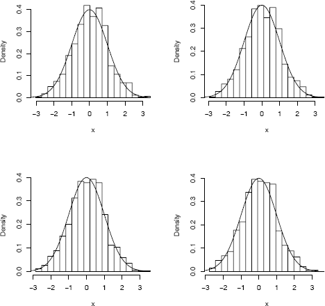
Histogram estimates of a normal sample with equal bin width but different bin origins, and standard normal density curve.
The Average Shifted Histogram (ASH) proposed by Scott [242] averages the density estimates. That is, the ASH estimate of density is
ˆfASH(x)=1m∑mj=1ˆfj(x),
where the class boundaries for estimate ˆfj+1(x) are shifted by h/m from the boundaries for ˆfj(x). Here we are viewing the estimates as m histograms with class width h. Alternately we can view the ASH estimate as a histogram with widths h/m. The optimal bin width (see [244, Sec. 5.2]) for the naive ASH estimate of a Normal(μ, σ2) density is
h*=2.576σn−1/5.(10.9)
Example 10.5 (Calculations for ASH estimate)
This numerical example illustrates the method of computing the ASH estimates. Four histogram estimates, each with bin width 1, are computed for a sample size n = 100. The bin origins for each of the densities are at 0, 0.25, 0.5, and 0.75 respectively. The bin counts and breaks are shown below.
breaks -4 -3 -2 -1 0 1 2 3 4
counts 0 2 11 27 38 16 6 0 4
breaks -3.75 -2.75 -1.75 -0.75 0.25 1.25 2.25 3.25 4.25
counts 0 4 17 23 38 16 2 0
breaks -3.5 -2.5 -1.5 -0.5 0.5 1.5 2.5 3.5 4.5
counts 0 7 21 23 34 15 0 0
breaks -3.25 -2.25 -1.25 -0.25 0.75 1.75 2.75 3.75 4.75
counts 2 9 26 30 21 12 0 0
To compute an ASH density estimate at the point x = 0.2, say, locate the intervals containing x = 0.2 and average these density estimates. The estimate is
ˆfASH(0.2)=14∑4K=1ˆfk(0.2)=14×38+23+23+30100(1)=114400=0.285.
Alternately, we can compute this estimate by considering the mesh over the subintervals with width δ = h/m = 0.25. There are now 36 breakpoints at −4 + 0.25i, i = 0, 1, ... , 35, and 35 bin counts, ν1, ... , ν35. The point x = 0.2 is in the intervals (−.75,.25], (−.5,.5], (−.25,.75], and (0, 1] corresponding to the 14th through 20th subintervals. The bin counts are
[1:12] 0 0 0 0 0 0 2 0 2 3 4 2
[13:24] 8 7 9 3 4 7 16 11 4 3 3 6
[25:35] 4 2 0 0 0 0 0 0 0 0 0
and the estimate can be computed by rearranging the terms as
7 + 9 + 3 + 4 = 23
9 + 3 + 4 + 7 = 23
3 + 4 + 7 + 16 = 30
4 + 7 + 16 + 11 = 38
= 7 + 2(9) + 3(3) + 4(4) + 3(7) + 2(16) + 11 = 114
or
ˆfASH(0.2)=v14+2v15+3v16+4v17+3v18+2v19+v20mnh
In general, if tk = max{tj : tj < x < tj+1}, we have
ˆfASH(x)=vk+1−m+2vk+2−m+...+mvk+...2vk+m−2+vk+m−1mnh =1nh∑m−1j=1−m(1−|j|n)vk+j. (10.10)
This computing formula requires that there are m − 1 empty bins on the left and the right. Equation (10.10) provides a formula for computing an ASH density estimate and shows that this estimate is a weighted average of the bin counts on the finer mesh. The weights (1 − |j|/m) correspond to a discrete triangular distribution on [−1, 1], which approaches the triangular density on [−1, 1] as m → ∞.
The ASH estimates can be generalized by replacing the weights (1− |j|/m) in (10.10) with a weight function w(j) = w(j, m) corresponding to a symmetric density supported on [−1, 1]. The triangular kernel is used in (10.10), which is
K(t)=1−|t|, |t|<1,
and K(t) = 0 otherwise. For other kernels see e.g. [244, 252] or the examples of density, and Section 10.2.
Example 10.6 (ASH density estimate)
Construct an ASH density estimate of the Old Faithful waiting time data in geyser$waiting (MASS) based on 20 histograms. For comparison with the naive histogram density estimate of this data in Example 10.3, the bin width is set to h = 7.27037. (The normal reference rule for ASH estimates in (10.9) gives h = 11.44258.)
library(MASS)
waiting <- geyser$waiting
n <- length(waiting)
m <- 20
a <- min(waiting) - .5
b <- max(waiting) + .5
h <- 7.27037
delta <- h / m
#get the bin counts on the delta-width mesh.
br <- seq(a - delta*m, b + 2*delta*m, delta)
histg <- hist(waiting, breaks = br, plot = FALSE)
nk <- histg$counts
K <- abs((1-m):(m-1))
fhat <- function(x) {
# locate the leftmost interval containing x
i <- max(which(x > br))
k <- (i - m + 1):(i + m - 1)
# get the 2m-1 bin counts centered at x
vk <- nk[k]
sum((1 - K / m) * vk) / (n * h) #f.hat
}
# density can be computed at any points in range of data
z <- as.matrix(seq(a, b + h, .1))
f.ash <- apply(z, 1, fhat) #density estimates at midpts
# plot ASH density estimate over histogram
br2 <- seq(a, b + h, h)
hist(waiting, breaks = br2, freq = FALSE, main = "",
ylim = c(0, max(f.ash)))
lines(z, f.ash, xlab = "waiting")
Compare the ASH estimate in Figure 10.5 with the histogram estimate in Figure 10.2(b) and the frequency polygon density estimate in Figure 10.3.

See the ash package [245] for an implementation of Scott’s univariate and bivariate ASH routines.
10.2 Kernel Density Estimation
Kernel density estimation generalizes the idea of a histogram density estimate. If a histogram with bin width h is constructed from a sample X1, ... , Xn, then a density estimate for a point x within the range of the data is
ˆf(x)=12hn×k,
where k is the number of sample points in the interval (x − h, x + h). This estimator can be written
ˆf(x)=1nn∑i=11hw(x−Xih), (10.11)
where w(t)=12I(|t|<1) is a weight function. The density estimator ˆf(x) in (10.11) with w(t)=12I(|t|<1) is called the naive density estimator. This weight function has the property that ∫1−1w(t)dt=1, and w(t) ≥ 0, so w(t) is a probability density supported on the interval [−1, 1].
Kernel density estimation replaces the weight function w(t) in the naive estimator with a function K(·) called a kernel function, such that
∫∞−∞K(t)dt=1.
In probability density estimation, K(·) is usually a symmetric probability density function. The weight function w(t)=12I(|t|<1) is called the rectangular kernel. The rectangular kernel is a symmetric probability density centered at the origin, and
1nhw(x−Xih),
corresponds to a rectangle of area 1/n centered at Xi. The density estimate at x is the sum of rectangles located within h units from x.
In this book, we restrict attention to symmetric positive kernel density estimators. Suppose that K(·) is another symmetric probability density centered at the origin, and define
ˆfK(x)=1n∑ni=11hK(x−Xih). (10.12)
Then ˆf is a probability density function. For example, K(x) may be the triangular density on [−1, 1] (the triangular kernel) or the standard normal density (the Gaussian kernel). In section Section 10.1.3 we have seen that the ASH density estimate converges to a triangular kernel density estimate (see equation (10.10) for the kernel) as n → ∞. The triangular kernel estimator corresponds to the sum of areas of triangles instead of rectangles. The Gaussian kernel estimator centers a normal density at each data point, as illustrated in Figure 10.6.

From the definition of the kernel density estimator in (10.12) it follows that certain continuity and differentiability properties of K(x) also hold for ˆfK(x). If K(x) is a probability density, then ˆfK(x) is continuous at x if K(x) is continuous at x, and ˆfK(x) has an rth order derivative at x if K(r)(x) exists. In particular, if K(x) is the Gaussian kernel, then ˆf is continuous and has derivatives of all orders.
The histogram density estimator corresponds to the rectangular kernel density estimator. The bin width h is a smoothing parameter; small values of h reveal local features of the density, while large values of h produce a smoother density estimate. In kernel density estimation h is called the bandwidth, smoothing parameter or window width.
The effect of varying the bandwidth is illustrated in Figure 10.6. The n = 10 sample points in Figure 10.6,
-0.77 -0.60 -0.25 0.14 0.45 0.64 0.65 1.19 1.71 1.74
were generated from the standard normal distribution. As the window width h decreases, the density estimate becomes rougher, and larger h corresponds to smoother density estimates. (This example is presented simply to graphically illustrate the kernel method; density estimation is not very useful for such a small sample.)
Table 10.2 gives some kernel functions that are commonly applied in density estimation, which are also shown in Figure 10.7. The Epanechnikov kernel was first suggested for kernel density estimation by Epanechnikov [85]. The efficiency of a kernel is defined by Silverman [252, p. 42]. The rescaled Epanechnikov kernel has efficiency 1, which is an optimal kernel in the sense of MISE (Scott [244, pp. 138–140]). The asymptotic relative efficiencies given in Table 10.2 in fact show that there is not much difference among the kernels if the mean integrated squared error criterion is used (see [252, p. 43]). See the examples of density for a method of calculating the efficiencies (actually the reciprocal of efficiency in Table 10.2).

Kernel Functions for Density Estimation
Kernel |
K(t) |
Support |
σ2K |
Efficiency |
Gaussian |
1√2πexp(−12t2) |
ℝ |
1 |
1.0513 |
Epanechnikov |
34(1−t2) |
|t|<1 |
1/5 |
1 |
Rectangular |
12 |
|t|<1 |
1/3 |
1.0758 |
Triangular |
1−|t| |
|t|<1 |
1/6 |
1.0143 |
Biweight |
1516(1−t2)2 |
|t|<1 |
1/7 |
1.0061 |
Cosine |
π4cosπ2t |
ℝ |
1-8/π2 |
1.0005 |
For a Gaussian kernel, the bandwidth h that optimizes IMSE is
h=(4/3)1/5σn−1/5=1.06σn−1/5. (10.13)
This choice of bandwidth is an optimal (IMSE) choice when the distribution is normal. If the true density is not unimodal, however, (10.13) will tend to oversmooth. Alternately, one can use a more robust estimate of dispersion in (10.13), setting
ˆσ=min(S,IQR/1.34),
where S is the standard deviation of the sample. Silverman [252, p. 48] indicates that an even better choice for a Gaussian kernel is the reduced width
h=0.9ˆσn−1/5=0.9min(S,IQR/1.34)n−1/5, (10.14)
which is a good starting point appropriate for a wide range of distributions that are not necessarily normal, unimodal, or symmetric.
The R reference manual [217] topic for bandwidth (?bw.nrd) refers to the rule in (10.14) as Silverman’s “rule-of-thumb,” which is applied unless the quartiles coincide. Various choices for bandwidth selection are illustrated in Examples 10.7 and 10.8 below.
For equivalent kernel rescaling, the bandwidth h1 can be rescaled by setting
h2≈σK1σK2h1.
Factors for equivalent smoothing are given by Scott [244, p. 142]. A kernel can also be scaled to “canonical” form such that the bandwidth is equivalent to the Gaussian kernel.
The density function in R computes kernel density estimates for seven kernels. The smoothing parameter is bw (bandwidth), but the kernels are scaled so that bw is the standard deviation of the kernel. The “canonical bandwidth” can be obtained using density with the option give.Rkern = TRUE. Choices for the kernel are gaussian, epanechnikov, rectangular, triangular, biweight, cosine, or optcosine. Run example(density) to see several plots of the corresponding density estimates. The cosine kernel given in Table 10.2 corresponds to the optcosine choice. The bandwidth adjustment for equivalent kernels in density is approximately 1, so the kernels are approximately equivalent.
Example 10.7 (Kernel density estimate of Old Faithful waiting time)
In this example we look at the result obtained by the default arguments to density. The default method applies the Gaussian kernel. For details on the default bandwidth selection see the help topics for bandwidth or bw.nrd0.
library(MASS)
waiting <- geyser$waiting
n <- length(waiting)
h1 <- 1.06 * sd(waiting) * n^(-1/5)
h2 <- .9 * min(c(IQR(waiting)/1.34, sd(waiting))) * n^(-1/5)
plot(density(waiting))
> print(density(waiting))
Call:
density.default(x = waiting)
Data: waiting (299 obs.); Bandwidth ‘bw’ = 3.998
x y
Min. : 31.01 Min. :3.762e-06
1st Qu.: 53.25 1st Qu.:4.399e-04
Median : 75.50 Median :1.121e-02
Mean : 75.50 Mean :1.123e-02
3rd Qu.: 97.75 3rd Qu.:1.816e-02
Max. :119.99 Max. :3.342e-02
sdK <- density(kernel = "gaussian", give.Rkern = TRUE)
> print(c(sdK, sdK * sd(waiting)))
[1] 0.2820948 3.9183881
> print(c(sd(waiting), IQR(waiting)))
[1] 13.89032 24.00000
> print(c(h1, h2))
[1] 4.708515 3.997796
The default density estimate applied the Gaussian kernel with the bandwidth h = 3.998 corresponding to equation (10.14). The default density plot with bandwidth 3.998 is shown in Figure 10.8. Other choices of bandwidth are also shown for comparison.

Gaussian kernel density estimates of Old Faithful waiting time in Example 10.7 using density with different bandwidths.
Example 10.8 (Kernel density estimate of precipitation data)
The dataset precip in R is the average amount of precipitation for 70 United States cities and Puerto Rico (see [217] for the source). We use the density function to construct kernel density estimates using the default and other choices for bandwidth.
n <- length(precip)
h1 <- 1.06 * sd(precip) * n^(-1/5)
h2 <- .9 * min(c(IQR(precip)/1.34, sd(precip))) * n^(-1/5)
h0 <- bw.nrd0(precip)
par(mfrow = c(2, 2))
plot(density(precip)) #default Gaussian (h0)
plot(density(precip, bw = h1)) #Gaussian, bandwidth h1
plot(density(precip, bw = h2)) #Gaussian, bandwidth h2
plot(density(precip, kernel = "cosine"))
par(mfrow = c(1,1))
The three values for bandwidth computed are
> print(c(h0, h1, h2))
[1] 3.847892 6.211802 3.847892
and the plots are shown in Figure 10.9. The default density plot applied the Gaussian kernel with the bandwidth h = 3.848 corresponding to equation (10.14) and the result of bw.nrd0.
Example 10.9 (Computing ˆf(x) for arbitrary x)
To estimate the density for new points, use approx.
d <- density(precip)
xnew <- seq(0, 70, 10)
approx(d$x, d$y, xout = xnew)
The code above produces the estimates:
$x
[1] 0 10 20 30 40 50 60 70
$y
[1] 0.000952360 0.010971583 0.010036739
[4] 0.021100536 0.035776120 0.014421428
[7] 0.005478733 0.001172337
For certain applications it is helpful to create a function to return the estimates, which can be accomplished easily with approxfun. Below fhat is a function returned by approxfun.
> fhat <- approxfun(d$x, d$y)
> fhat(xnew)
[1] 0.000952360 0.010971583 0.010036739
[4] 0.021100536 0.035776120 0.014421428
[7] 0.005478733 0.001172337
Boundary kernels
Near the boundaries of the support set of a density, or discontinuity points, kernel density estimates have larger errors. Kernel density estimates tend to smooth the probability mass over the discontinuity points or boundary points. For example, see the kernel density estimates of the precipitation data shown in Figure 10.9. Note that the density estimates suggest that negative inches of precipitation are possible.

Kernel density estimates of precipitation data in Example 10.8 using density with different bandwidths.
In the next example, we illustrate the boundary problem with an exponential density, and compare the kernel estimate with the true density.
Example 10.10 (Exponential density)
A Gaussian kernel density estimate of an Exponential(1) density is shown in Figure 10.10. The true exponential density is shown with a dashed line.

Gaussian kernel density estimate (solid line) of an exponential density in Example 10.10, with true density (dashed line). In the second plot, the reflection boundary technique is applied on the same data.
x <- rexp(1000, 1)
plot(density(x), xlim = c(-1, 6), ylim = c(0, 1), main="")
abline(v = 0)
# add the true density to compare
y <- seq(.001, 6, .01)
lines(y, dexp(y, 1), lty = 2)
Note that the smoothness of the kernel estimate does not fit the discontinuity of the density at x = 0.
Scott [244] discusses boundary kernels, which are finite support kernels that are applied to obtain the density estimate in the boundary region. A simple fix is to use a reflection boundary technique if the discontinuity occurs at the origin. First add the reflection of the entire sample; that is, append −x1, ... , −xn to the data. Then estimate a density g using the 2n points, but use n to determine the smoothness parameter. Then ˆf(x)=2ˆg(x). This method is applied below.
Example 10.11 (Reflection boundary technique)
The reflection boundary technique can be applied when the density has a discontinuity at 0, such as in Example 10.10.
xx <- c(x, -x)
g <- density(xx, bw = bw.nrd0(x))
a <- seq(0, 6, .01)
ghat <- approx(g$x, g$y, xout = a)
fhat <- 2 * ghat$y # density estimate along a
bw <- paste("Bandwidth = ", round(g$bw, 5))
plot(a, fhat, type="l", xlim=c(-1, 6), ylim=c(0, 1),
main = "", xlab = bw, ylab = "Density")
abline(v = 0)
# add the true density to compare
y <- seq(.001, 6, .01)
lines(y, dexp(y, 1), lty = 2)
The plot of the density estimate with reflection boundary is shown in Figure 10.10.
See Scott [244] or Wand and Jones [289] for further discussion of methods for kernel density estimation near boundaries.
10.3 Bivariate and Multivariate Density Estimation
In this section examples are presented that illustrate some of the basic methods for bivariate and multivariate density estimation. Scott [244] is a comprehensive reference on multivariate density estimation. Also see Silverman [252, Ch. 4].
10.3.1 Bivariate Frequency Polygon
To construct a bivariate density histogram (polygon), it is necessary to define two-dimensional bins and count the number of observations in each bin. The bin2d function in the following example computes the two dimensional frequency table.
Example 10.12 (Bivariate frequency table: bin2d)
The function bin2d bins a bivariate data matrix, based on the univariate histogram hist in R. See the documentation for hist for an explanation of how the breakpoints are determined.
The frequencies are computed by constructing a two dimensional contingency table with the marginal breakpoints as the cut points. The return value of bin2d is a list including the table of bin frequencies, vectors of breakpoints, and vectors of midpoints.
bin2d <-
function(x, breaks1 = "Sturges", breaks2 = "Sturges"){
# Data matrix x is n by 2
# breaks1, breaks2: any valid breaks for hist function
# using same defaults as hist
histg1 <- hist(x[,1], breaks = breaks1, plot = FALSE)
histg2 <- hist(x[,2], breaks = breaks2, plot = FALSE)
brx <- histg1$breaks
bry <- histg2$breaks
# bin frequencies
freq <- table(cut(x[,1], brx), cut(x[,2], bry))
return(list(call = match.call(), freq = freq,
breaks1 = brx, breaks2 = bry,
mids1 = histg1$mids, mids2 = histg2$mids))
}
To show the details of the bin2d function, it is applied to bin the bivariate sepal length and sepal width distribution of iris setosa data. Then in Example 10.13 bin2d is used to bin data for constructing a bivariate frequency polygon.
> bin2d(iris[1:50,1:2])
$call bin2d(x = iris[1:50, 1:2])
$freq
(2,2.5] (2.5,3] (3,3.5] (3.5,4] (4,4.5]
(4.2,4.4] 0 3 1 0 0
(4.4,4.6] 1 0 3 1 0
(4.6,4.8] 0 2 5 0 0
(4.8,5] 0 2 8 2 0
(5,5.2] 0 0 6 4 1
(5.2,5.4] 0 0 2 4 0
(5.4,5.6] 0 0 1 0 1
(5.6,5.8] 0 0 0 2 1
$breaks1
[1] 4.2 4.4 4.6 4.8 5.0 5.2 5.4 5.6 5.8
$breaks2
[1] 2.0 2.5 3.0 3.5 4.0 4.5
$mids1
[1] 4.3 4.5 4.7 4.9 5.1 5.3 5.5 5.7
$mids2
[1] 2.25 2.75 3.25 3.75 4.25
Example 10.13(Bivariate density polygon)
Bivariate data is displayed in a 3D density polygon, using the bin2d function in Example 10.12 to compute the bivariate frequency table. After binning the bivariate data, the persp function plots the density polygon.
#generate standard bivariate normal random sample
n <- 2000; d <- 2
x <- matrix(rnorm(n*d), n, d)
# compute the frequency table and density estimates
b <- bin2d(x)
h1 <- diff(b$breaks1)
h2 <- diff(b$breaks2)
# matrix h contains the areas of the bins in b
h <- outer(h1, h2, "*")
Z <- b$freq / (n * h) # the density estimate
persp(x=b$mids1, y=b$mids2, z=Z, shade=TRUE,
xlab="X", ylab="Y", main="",
theta=45, phi=30, ltheta=60)
The perspective plot, a three dimensional density polygon, is shown in Figure 10.11. Also see Figure 4.7 on page 109 for another view of bivariate normal data, in a "flat" hexagonal histogram.

Density polygon of bivariate normal data in Example 10.13, using normal reference rule (Sturges’ Rule) to determine bin widths.
See the persp examples for more options, including color. Also see the wireframe function in the lattice [239] package. Other functions that bin bivariate data are e.g. bin2 (ash) [245] and hist2d (gplots) [290].
3D Histogram
A 3D histogram can be displayed by functions in the rgl [2] package, an interactive 3D graphics package. To see a demo, type
library(rgl)
demo(hist3d)
After running the demo, the source code for two functions named hist3d and binplot.3d that are used in the demo should have appeared in the console window (scroll up to see it). To apply the rgl demo histogram to this example, copy the two functions hist3d and binplot.3d into a source file. These functions are in the file hist3d.r located in the demo directory of library/rgl.
library(rgl)
#run demo(hist3d) or
#source binplot.3d and hist3d functions
n <- 1000
d <- 2
x <- matrix(rnorm(n*d), n, d)
rgl.clear()
hist3d(x[,1], x[,2])
As Silverman [252, p. 78] points out, there are serious presentational difficulties with a 3D histogram. The surface and wireframe plots of bivariate densities are better, particularly when they are generated from a continuous density estimator.
10.3.2 Bivariate ASH
The average shifted histogram estimator of density can be extended to multivariate density estimation. Suppose that bivariate data {(x, y)}, have been sorted into an nbin1 by nbin2 array of bins with frequencies v = (vij) and bin widths h = (h1, h2) (see e.g. the bin2d function in Example 10.12). The parameter m = (m1, m2) is the number of shifted histograms on each axis used in the estimate. The histograms are shifted in two directions, so that there are m1m2 histogram density estimates to be averaged.
The bivariate ASH estimate of the joint density f(x, y) is
ˆfASH(x,y)=1m1m2m1∑i=1m2∑j=1ˆfij(x,y).
The bin weights are given by
One can apply a similar algorithm for computing the individual estimates as in the univariate ASH. See Scott [244, Sec. 5.2] for a bivariate ASH algorithm. The ASH estimates can be generalized by replacing the weights and in (10.15) with other kernels. The triangular kernel is applied in (10.15). Also note that the bivariate ASH methods can be generalized to dimension d ≥ 2.
Example 10.14 (Bivariate ASH density estimate)
This example computes a bivariate ASH estimate of a bivariate normal sample, using Scott’s routines in the ash package [245]. The function ash2 returns a list containing (among other things) the coordinates of the bin centers and the density estimates, labeled x, y, z. The generator rmvn.eigen is given in Example 3.16 on page 71. Alternately, samples can be generated using e.g. mvrnorm (MASS).
library(ash) # for bivariate ASH density est.
# generate N_2(0,Sigma) data
n <- 2000
d <- 2
nbin <- c(30, 30) # number of bins
m <- c(5, 5) # smoothing parameters
# First example with positive correlation
Sigma <- matrix(c(1, .9, .9, 1), 2, 2)
set.seed(345)
x <- rmvn.eigen(n, c(0, 0), Sigma=Sigma)
b <- bin2(x, nbin = nbin)
# kopt is the kernel type, here triangular
est <- ash2(b, m = m, kopt = c(1,0))
persp(x = est$x, y = est$y, z = est$z, shade=TRUE,
xlab = "X", ylab = "Y", zlab = "", main="",
theta = 30, phi = 75, ltheta = 30, box = FALSE)
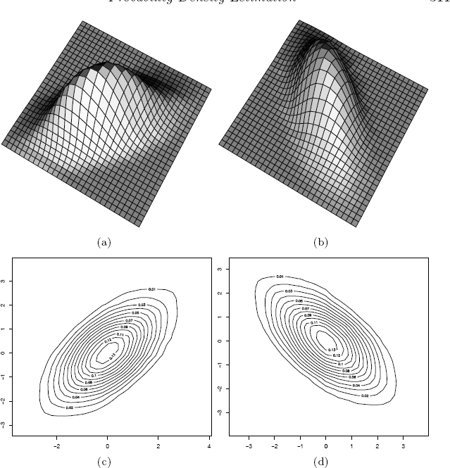
contour(x = est$x, y = est$y, z = est$z, main="")
The perspective and contour plots from the ASH estimates are shown in Figures 10.12(a) and 10.12(c). The variables in the first example have positive correlation ρ = 0.9. In the second example, the variables have negative correlation ρ = −0.9.
# Second example with negative correlation
Sigma <- matrix(c(1, -.9, -.9, 1), 2, 2)
set.seed(345)
x <- rmvn.eigen(n, c(0, 0), Sigma=Sigma)
b <- bin2(x, nbin = nbin)
est <- ash2(b, m = m, kopt = c(1,0))
persp(x = est$x, y = est$y, z = est$z, shade=TRUE,
xlab = "X", ylab = "Y", zlab = "", main="",
theta = 30, phi = 75, ltheta = 30, box = FALSE)
contour(x = est$x, y = est$y, z = est$z, main="")
par(ask = FALSE)
The perspective plots and contour plots from the ASH estimates of the densities in the second case are shown in Figures 10.12(b) and 10.12(d).
10.3.3 Multidimensional kernel methods
Suppose X = (X1,..., Xd) is a random vector in ℝd, and K(X) : ℝd → ℝ is a kernel function, such that K(X) is a density function on ℝd. Let the n × d matrix (xij) be an observed sample from the distribution of X. The smoothing parameter is a d-dimensional vector h. If the bandwidth is equal in all dimensions, the multivariate kernel density estimator of f(X) with smoothing parameter h1 is
where xi. is the ith row of (xij). Usually K(X) will be a symmetric and unimodal density on ℝd, such as a standard multivariate normal density. The Gaussian kernels have unbounded support. An example of a kernel with bounded support is the multivariate version of the Epanechnikov kernel, defined
where cd = 2πd/2/(dΓ(d/2)) is the volume of the d-dimensional unit sphere. When d = 1 the constant is c1 = 2 and K(x) = (3/4)(1−x2) I(|x| < 1), which is the univariate Epanechnikov kernel given in Table 10.2.
In the bivariate case, choosing equal bandwidths h1 = h2 and the standard Gaussian kernel corresponds to centering identical weight functions like smooth bumps at each sample point and summing the heights of these surfaces to obtain the density estimate at a given point. For the bivariate Gaussian kernel, in a graphical representation corresponding to Figure 10.6 the small bumps will be surfaces (bivariate normal densities) rather than curves.
The product kernel density estimate of f(X) with smoothing parameter h = (h1,..., hd) is
For this estimator and the multivariate frequency polygon, the optimal smoothing parameter has
and for uncorrelated multivariate normal data the optimal bandwidths are
The constant (4/(d + 2))1/(d+4) is close to 1 and converges to 1 as d → ∞, thus Scott’s multivariate normal reference rule [244] for d-dimensional data is
Example 10.15 (Product kernel estimate of a bivariate normal mixture)
This example plots the density estimate for a bivariate normal location mixture using kde2d (MASS). The mixture has three components with different mean vectors and identical variance ∑ = I2. The mean vectors are
and the mixing probabilities are p = (0.2, 0.3, 0.5). The code to generate the mixture data and plots in Figure 10.13 follows.

Product kernel estimates of bivariate normal mixture data in Example 10.15 (normal reference rule at left.)
library(MASS) #for mvrnorm and kde2d
#generate the normal mixture data
n <- 2000
p <- c(.2, .3, .5)
mu <- matrix(c(0, 1, 4, 0, 3, -1), 3, 2)
Sigma <- diag(2)
i <- sample(1:3, replace = TRUE, prob = p, size = n)
k <- table(i)
x1 <- mvrnorm(k[1], mu = mu[1,], Sigma)
x2 <- mvrnorm(k[2], mu = mu[2,], Sigma)
x3 <- mvrnorm(k[3], mu = mu[3,], Sigma)
X <- rbind(x1, x2, x3) #the mixture data
x <- X[,1]
y <- X[,2]
> print(c(bandwidth.nrd(x), bandwidth.nrd(y)))
[1] 1.876510 1.840368
# accepting the default normal reference bandwidth
fhat <- kde2d(x, y)
contour(fhat)
persp(fhat, phi = 30, theta = 20, d = 5, xlab = "x")
# select bandwidth by unbiased cross-validation
h = c(ucv(x), ucv(y))
fhat <- kde2d(x, y, h = h)
contour(fhat)
persp(fhat, phi = 30, theta = 20, d = 5, xlab = "x")
The bandwidth by normal reference is h ≐ (1.877, 1.840), and by cross-validation h ≐ (0.556, 1.132). The first choice results in a smoother estimate. Although in Figure 10.13 three modes are evident for both estimates, it appears that the density estimate corresponding to unbiased cross-validation may be too rough in this example.
For kernel density estimates for multivariate data also see kde (ks) [76] and KernSnooth [286]. Readers are referred to the examples of kde2d (MASS) for a Gaussian kernel density estimate of the bivariate geyser (MASS) data with default normal reference bandwidth (also see [278, 5.6]).
10.4 Other Methods of Density Estimation
Orthogonal systems provide an alternate approach to density estimation [244, 252, 285]. Suppose that the random variable X is supported on the interval [0, 1]. Then one approach to estimation of the density f of X is to represent f by its Fourier expansion and estimate the Fourier coefficients from the observed random sample X1,..., Xn. Although intuitively appealing, the resulting estimator is not useful because it will tend to a sum of delta functions that place probability mass at the individual observations. See [244], [252], or [285] for an explanation of how this problem is resolved by smoothing to obtain a more useful density estimator, and how it is generalized to densities with unbounded support. Scott [244, p. 129] shows that the resulting estimator is in the form of a fixed kernel estimator. Walter and Shen [285, Sec. 13.3] show that an estimator based on the Haar wavelets is the traditional histogram estimator of a density.
Scott [244] and Silverman [252] discuss several other approaches to density estimation including adaptive kernel methods and cross-validation, near neighbor estimates, and penalized likelihood methods. An L1 approach to density estimation is covered by Devroye and Györfi [71]. Many other criteria have been applied, such as the Kullback-Liebler distance, Hellinger distance, AIC, etc. Other approaches focus on regression and smoothing [79, 128, 129, 130, 203], splines [86, 284], or generalized additive models [135, 137]. Some related R packages are ash [245], gam [134], gss [123], KernSmooth [286], ks [76], locfit [180], MASS [278], sm [29], and splines.
Exercises
10.1 Construct a histogram estimate of density for a random sample of standard lognormal data using Sturges’ Rule, for sample size n = 100. Repeat the estimate for the same sample using the correction for skewness proposed by Doane [73] in equation (10.2). Compare the number of bins and break points using both methods. Compare the density estimates at the deciles of the lognormal distribution with the lognormal density at the same points. Does the suggested correction give better density estimates in this example?
10.2 Estimate the IMSE for three histogram density estimates of standard normal data, from a sample size n = 500. Use Sturges’ Rule, Scott’s Normal Reference Rule, and the FD Rule.
10.3 Construct a frequency polygon density estimate for the precip dataset in R. Verify that the estimate satisfies by numerical integration of the density estimate.
10.4 Construct a frequency polygon density estimate for the precip dataset, using a bin width determined by substituting
for standard deviation in the usual Normal Reference Rule for a frequency polygon.
10.5 Construct a frequency polygon density estimate for the precip dataset, using a bin width determined by the Normal Reference Rule for a frequency polygon adjusted for skewness. The skewness adjustment factor is given in 10.8.
10.6 Construct an ASH density estimate for the faithful$eruptions dataset in R, using width h determined by the normal reference rule. Use a weight function corresponding to the biweight kernel,
10.7 Construct an ASH density estimate for the precip dataset in R. Choose the best value for width h* empirically by computing the estimates over a range of possible values of h and comparing the plots of the densities. Does the optimal value correspond to the optimal value h* suggested by comparing the density plots?
- 10.8 The buffalo dataset in the gss [123] package contains annual snowfall accumulations in Buffalo, New York from 1910 to 1973. The 64 observations are
126.4 82.4 78.1 51.1 90.9 76.2 104.5 87.4 110.5 25.0 69.3 53.5 39.863.6 46.7 72.9 79.6 83.6 80.7 60.3 79.0 74.4 49.6 54.7 71.8 49.1103.9 51.6 82.4 83.6 77.8 79.3 89.6 85.5 58.0 120.7 110.5 65.4 39.940.1 88.7 71.4 83.0 55.9 89.9 84.8 105.2 113.7 124.7 114.5 115.6 102.4101.4 89.8 71.5 70.9 98.3 55.5 66.1 78.4 120.5 97.0 110.0This data was analyzed by Scott [242]. Construct kernel density estimates of the data using Gaussian and biweight kernels. Compare the estimates for different choices of bandwidth. Is the estimate more influenced by the type of kernel or the bandwidth?
10.9 Construct a kernel density estimate for simulated data from the normal location mixture . Compare several choices of bandwidth, including (10.13) and (10.14). Plot the true density of the mixture over the density estimate, for comparison. Which choice of smoothing parameter appears to be best?
10.10 Apply the reflection boundary technique to obtain a better kernel density estimate for the precipitation data in Example 10.8. Compare the estimates in Example 10.8 and the improved estimates in a single graph. Also try setting from = 0 or cut = 0 in the density function.
10.11 Write a bivariate density polygon plotting function based on Examples 10.12 and 10.13. Use Example 10.13 to check the results, and then apply your function to display the bivariate faithful data (Old Faithful geyser).
10.12 Plot a bivariate ASH density estimate of the geyser(MASS) data.
10.13 Generalize the bivariate ASH algorithm to compute an ASH density estimate for a d-dimensional multivariate density, d ≥ 2.
10.14 Write a function to bin three-dimensional data into a three-way contingency table, following the method in the bin2d function of Example 10.12. Check the result on simulated N3(0, I) data. Compare the marginal frequencies returned by your function to the expected frequencies from a standard univariate normal distribution.
R Code
Code to generate data as shown in Table 10.1 on page 289.
N <- c(10, 20, 30, 50, 100, 200, 500, 1000, 5000, 10000)
m <- length(N)
out <- matrix(0, nrow = m, ncol = 8)
out[,1] <- N
out[,5] <- N
for (i in 1:m) {
x <- rnorm(N[i])
out[i, 2:4] <- c(nclass.Sturges(x),
nclass.scott(x), nclass.FD(x))
x <- rexp(N[i])
out[i, 6:8] <- c(nclass.Sturges(x),
nclass.scott(x), nclass.FD(x))
}
print(out)
Code to plot the histograms in Figure 10.4 on page 294.
library(MASS) #for truehist
par(mfrow = c(2, 2))
x <- sort(rnorm(1000))
y <- dnorm(x)
o <- (1:4) / 4
h <- .35
for (i in 1:4) {
truehist(x, prob = TRUE, h = .35, x0 = o[i],
xlim = c(-3.5, 3.5), ylim = c(0, 0.45),
ylab = "Density", main = "")
lines(x, y)
}
par(mfrow = c(1, 1))
Code to plot Figure 10.6 on page 298.
To display the type of plot in Figure 10.6, first open a new plot to set up the plotting window, but use type="n” in the plot command so that nothing is drawn in the graph window yet. Then add the density curves for each point inside the loop using lines. Finally, add the density estimate using lines again.
for (h in c(.25, .4, .6, 1)) {
x <- seq(-4, 4, .01)
fhat <- rep(0, length(x))
# set up the plot window first
plot(x, fhat, type="n", xlab="", ylab="",
main=paste("h=",h), xlim=c(-4,4), ylim=c(0, .5))
for (i in 1:n) {
# plot a normal density at each sample pt
z <- (x - y[i]) / h
f <- dnorm(z)
lines(x, f / (n * h))
# sum the densities to get the estimates
fhat <- fhat + f / (n * h)
}
lines(x, fhat, lwd=2) # add density estimate to plot
}
Use par(mfrow = c(2, 2)) to display four plots in one screen.
Code to plot kernels in Figure 10.7 on page 299.
#see examples for density, kernels in S parametrization
(kernels <- eval(formals(density.default)$kernel))
plot(density(0, from=-1.2, to=1.2, width=2,
kern="gaussian"), type="l", ylim=c(0, 1),
xlab="", main="")
for(i in 2:5)
lines(density(0, width=2, kern=kernels[i]), lty=i)
legend("topright", legend=kernels[1:5],
lty=1:5, inset=.02)