Chapter 7

Bootstrap and Jackknife

7.1 The Bootstrap

The bootstrap was introduced in 1979 by Efron [80], with further developments in 1981 [82, 81], 1982 [83], and numerous other publications including the monograph of Efron and Tibshirani [84]. Chernick [45] has an extensive bibliography. Davison and Hinkley [63] is a comprehensive reference with many applications. Also see Barbe and Bertail [19], Shao and Tu [247], and Mammen [186].

Bootstrap methods are a class of nonparametric Monte Carlo methods that estimate the distribution of a population by resampling. Resampling methods treat an observed sample as a finite population, and random samples are generated (resampled) from it to estimate population characteristics and make inferences about the sampled population. Bootstrap methods are often used when the distribution of the target population is not specified; the sample is the only information available.

The term “bootstrap” can refer to nonparametric bootstrap or parametric bootstrap. Monte Carlo methods that involve sampling from a fully specified probability distribution, such as methods of Chapter 6 are sometimes called parametric bootstrap. Nonparametric bootstrap is the subject of this chapter. In nonparametric bootstrap, the distribution is not specified.

The distribution of the finite population represented by the sample can be regarded as a pseudo-population with similar characteristics as the true population. By repeatedly generating random samples from this pseudo-population (resampling), the sampling distribution of a statistic can be estimated. Properties of an estimator such as bias or standard error can be estimated by resampling.

Bootstrap estimates of a sampling distribution are analogous to the idea of density estimation. We construct a histogram of a sample to obtain an estimate of the shape of the density function. The histogram is not the density, but in a nonparametric problem, can be viewed as a reasonable estimate of the density. We have methods to generate random samples from completely specified densities; bootstrap generates random samples from the empirical distribution of the sample.

Suppose that x = (x1, ... , xn) is an observed random sample from a distribution with cdf F(x). If X* is selected at random from x, then

$\begin{array}{cc}P\left(X^{*}=x_i\right)=\frac{1}{n},& i=1,...,n.\end{array}$

Resampling generates a random sample $X_1^{*},...,X_n^{*}$ by sampling with replacement from x. The random variables $X_i^{*}$ are iid, uniformly distributed on the set {x1, ... , xn}.

The empirical distribution function (ecdf) Fn(x) is an estimator of F(x). It can be shown that Fn(x) is a sufficient statistic for F(x); that is, all the information about F(x) that is contained in the sample is also contained in Fn(x). Moreover, Fn(x) is itself the distribution function of a random variable; namely the random variable that is uniformly distributed on the set {x1, ... , xn}. Hence the empirical cdf Fn is the cdf of X*. Thus in bootstrap, there are two approximations. The ecdf Fn is an approximation to the cdf FX. The ecdf $F_m^{*}$ of the bootstrap replicates is an approximation to the ecdf Fn. Resampling from the sample x is equivalent to generating random samples from the distribution Fn(x). The two approximations can be represented by the diagram

$\begin{array}{c}F\to X\to F_n\\ F_n\to X^{*}\to F_n^{*}.\end{array}$

To generate a bootstrap random sample by resampling x, generate n random integers {i1, ... , in} uniformly distributed on {1, ... , n} and select the bootstrap sample $x^{*}=\left(x_{i_1},...,x_{i_n}\right)$.

Suppose θ is the parameter of interest (θ could be a vector), and $\widehat{\theta }$ is an estimator of θ. Then the bootstrap estimate of the distribution of $\widehat{\theta }$ is obtained as follows.

1. For each bootstrap replicate, indexed b = 1, ... , B:
   1. Generate sample $x^{*\left(b\right)}=x_1^{*},...,x_n^{*}$ by sampling with replacement from the observed sample x1, ... , xn.
   2. Compute the bth replicate ${\widehat{\theta }}^{\left(b\right)}$ from the bth bootstrap sample.
2. The bootstrap estimate of $F_{\widehat{\theta }}(\cdot )$ is the empirical distribution of the replicates ${\widehat{\theta }}^{(1)},...,{\widehat{\theta }}^{(B)}$.

The bootstrap is applied to estimate the standard error and the bias of an estimator in the following sections. First let us see an example to illustrate the relation between the ecdf Fn and the distribution of the bootstrap replicates.

Example 7.1 (Fn and bootstrap samples)

Suppose that we have observed the sample

$x\text{ = }\left\{\text{2, 2, 1, 1, 5, 4, 4, 3, 1, 2}\right\}\text{.}$

Resampling from x we select 1, 2, 3, 4, or 5 with probabilities 0.3, 0.3, 0.1, 0.2, and 0.1 respectively, so the cdf FX* of a randomly selected replicate is exactly the ecdf Fn(x):

$F_{X*}\left(x\right)=F_n\left(x\right)=\{\begin{array}{cc}0,& x<1;\\ 0.3,& 1\le x\le 2;\\ 0.6,& 2\le x\le 3;\\ 0.7,& 3\le x\le 4;\\ 0.9,& 4\le x\le 5;\\ 1,& x\ge 5.\end{array}$

Note that if Fn is not close to FX then the distribution of the replicates will not be close to FX. The sample x above is actually a sample from a Poisson(2) distribution. Resampling from x a large number of replicates produces a good estimate of Fn but not a good estimate of FX, because regardless of how many replicates are drawn, the bootstrap samples will never include 0.

7.1.1 Bootstrap Estimation of Standard Error

The bootstrap estimate of standard error of an estimator $\widehat{\theta }$ is the sample standard deviation of the bootstrap replicates ${\widehat{\theta }}^{(1)},...,{\widehat{\theta }}^{(B)}$.

$\begin{array}{cc}\widehat{se}\left({\widehat{\theta }}^{*}\right)=\sqrt{\frac{1}{B-1}{\displaystyle \sum _{b=1}^B{\left({\widehat{\theta }}^{(b)}-\overline{{\widehat{\theta }}^{*}}\right)}^2,}}& \left(7.1\right)\end{array}$

where $\overline{{\widehat{\theta }}^{*}}=\frac{1}{B}{\displaystyle \sum }_{b=1}^B{\widehat{\theta }}^{(b)}$ [84, (6.6)].

According to Efron and Tibshirani [84, p. 52], the number of replicates needed for good estimates of standard error is not large; B = 50 is usually large enough, and rarely is B > 200 necessary. (Much larger B will be needed for confidence interval estimation.)

Example 7.2 (Bootstrap estimate of standard error)

The law school data set law in the bootstrap [271] package is from Efron and Tibshirani [84]. The data frame contains LSAT (average score on law school admission test score) and GPA (average undergraduate grade-point average) for 15 law schools.

 LSAT 576 635 558 578 666 580 555 661 651 605 653 575 545 572 594

 GPA 339 330 281 303 344 307 300 343 336 313 312 274 276 288 296

This data set is a random sample from the universe of 82 law schools in law82 (bootstrap). Estimate the correlation between LSAT and GPA scores, and compute the bootstrap estimate of the standard error of the sample correlation.

1. For each bootstrap replicate, indexed b = 1, ... , B:
   1. Generate sample $x^{*\left(b\right)}=x_1^{*},...,x_n^{*}$ by sampling with replacement from the observed sample x1, ... , xn.
   2. Compute the bth replicate ${\widehat{\theta }}^{(b)}$ from the bth bootstrap sample, where $\widehat{\theta }$ is the sample correlation R between (LSAT, GPA).
2. The bootstrap estimate of se(R) is the sample standard deviation of the replicates ${\widehat{\theta }}^{(1)},...,{\widehat{\theta }}^{(B)}=R^{(1)},...,R^{(B)}$.

  library(bootstrap) #for the law data

  print(cor(law$LSAT, law$GPA))

  [1] 0.7763745

  print(cor(law82$LSAT, law82$GPA))

  [1] 0.7599979

The sample correlation is R = 0.7763745. The correlation for the universe of 82 law schools is R = 0.7599979. Use bootstrap to estimate the standard error of the correlation statistic computed from the sample of scores in law.

  #set up the bootstrap

  B <- 200   #number of replicates

  n <- nrow(law)  #sample size

  R <- numeric(B) #storage for replicates

  #bootstrap estimate of standard error of R

  for (b in 1:B) {

  #randomly select the indices

  i <- sample(1:n, size = n, replace = TRUE)

  LSAT <- law$LSAT[i]  #i is a vector of indices

  GPA <- law$GPA[i]

  R[b] <- cor(LSAT, GPA)

 }

  #output

  > print(se.R <- sd(R))

  [1] 2.1358393

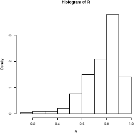
  > hist(R, prob = TRUE)

The bootstrap estimate of se(R) is 0.1358393. The normal theory estimate for standard error of R is 0.115. The jackknife-after-bootstrap method of estimating $\widehat{se}\left(\widehat{se}\left(\widehat{\theta }\right)\right)$ is covered in Section 7.3. The histogram of the replicates of R is shown in Figure 7.1.

In the next example, the boot function in recommended package boot [34] is applied to run the bootstrap. See Appendix B.1 for a note about how to write the function for the statistic argument in boot.

Example 7.3 (Bootstrap estimate of standard error: boot function)

Example 7.2 is repeated, using the boot function in boot. First, write a function that returns ${\widehat{\theta }}^{(b)}$, where the first argument to the function is the sample data, and the second argument is the vector {i1, ... , in} of indices. If the data is x and the vector of indices is i, we need x[i,1] to extract the first resampled variable, and x[i,2] to extract the second resampled variable. The code and output is shown below.

  r <- function(x, i) {

  #want correlation of columns 1 and 2

  cor(x[i,1], x[i,2])

 }

The printed summary of output from the boot function is obtained by the command boot or the result can be saved in an object for further analysis. Here we save the result in obj and print the summary.

  library(boot)  #for boot function

  > obj <- boot(data = law, statistic = r, R = 2000)

  > obj

  ORDINARY NONPARAMETRIC BOOTSTRAP

  Call: boot(data = law, statistic = r, R = 2000)

  Bootstrap Statistics :

   original  bias std. error

  t1* 0.7763745 -0.004795305  0.1303343

The observed value $\widehat{\theta }$ of the correlation statistic is labeled t1*. The bootstrap estimate of standard error of the estimate is $\widehat{se}\left(\widehat{\theta }\right)\doteq 0.13,$ based on 2000 replicates. To compare with formula (7.1), extract the replicates in $t.

  > y <- obj$t

  > sd(y)

  [1] 0.1303343

R note 7.1 The syntax and options for the boot (boot) function and the bootstrap (bootstrap) function are different. Note that the bootstrap package [271] is a collection of functions and data for the book by Efron and Tibshirani [84], and the boot package [34] is a collection of functions and data for the book by Davison and Hinkley [63].

7.1.2 Bootstrap Estimation of Bias

If $\widehat{\theta }$ is an unbiased estimator of θ, $E[\widehat{\theta }]=\theta .$ The bias of an estimator $\widehat{\theta }$ for θ

$bias(\widehat{\theta })=E[\widehat{\theta }-\theta ]=E[\widehat{\theta }]-\theta .$

Thus, every statistic is an unbiased estimator of its expected value, and in particular, the sample mean of a random sample is an unbiased estimator of the mean of the distribution. An example of a biased estimator is the maximum likelihood estimator of variance, ${\widehat{\sigma }}^2=\frac{1}{n}{\displaystyle {\sum }_{i=1}^n{\left(X_i-\overline{X}\right)}^2,}$ which has expected value $\left(1-1/n\right){\sigma }^2.$ Thus, ${\widehat{\sigma }}^2$ underestimates ${\sigma }^2,$ and the bias is $\raisebox{1ex}{$-{\sigma }^2$}\!\left/ \!\raisebox{-1ex}{$n$}\right.$.

The bootstrap estimation of bias uses the bootstrap replicates of $\widehat{\theta }$ to estimate the sampling distribution of $\widehat{\theta }.$ For the finite population x = (x1,... , xn), the parameter is $\widehat{\theta }(x)$ and there are B independent and identically distributed estimators ${\widehat{\theta }}^{(b)}$. The sample mean of the replicates $\left\{{\widehat{\theta }}^{(b)}\right\}$ is unbiased for its expected value $E[{\widehat{\theta }}^{*}],$ so the bootstrap estimate of bias is

$\begin{array}{cc}\widehat{bias}(\widehat{\theta })=\overline{{\widehat{\theta }}^{*}}-\widehat{\theta },& \left(7.2\right)\end{array}$

where $\overline{\widehat{\theta }*}=\frac{1}{B}{\displaystyle {\sum }_{b=1}^B{\widehat{\theta }}^{(b)}},$ and $\widehat{\theta }=\widehat{\theta }(x)$ is the estimate computed from the original observed sample. (In bootstrap Fn is sampled in place of FX, so we replace θ with $\widehat{\theta }$ to estimate the bias.) Positive bias indicates that $\widehat{\theta }$ on average tends to overestimate θ.

Example 7.4 (Boostrap estimate of bias)

In the law data of Example 7.2, compute the bootstrap estimate of bias in the sample correlation.

  #sample estimate for n=15

  theta.hat <- cor(law$LSAT, law$GPA)

  #bootstrap estimate of bias

  B <- 2000  #larger for estimating bias 

  n <- nrow(law)

  theta.b <- numeric(B)

  for (b in 1:B) {

  i <- sample(1:n, size = n, replace = TRUE)

  LSAT <- law$LSAT[i]

  GPA <- law$GPA[i]

  theta.b[b] <- cor(LSAT, GPA)

 }

  bias <- mean(theta.b - theta.hat)

  > bias

  [1] -0.005797944

The estimate of bias is -0.005797944. Note that this is close to the estimate of bias returned by the boot function in Example 7.3. See Section 7.3 for the jackknife-after-bootstrap method to estimate the standard error of the bootstrap estimate of bias.

Example 7.5 (Bootstrap estimate of bias of a ratio estimate)

The patch (bootstrap) data from Efron and Tibshirani [84, 10.3] contains measurements of a certain hormone in the bloodstream of eight subjects after wearing a medical patch. The parameter of interest is

$\theta =\frac{E\left(new\right)-E\left(old\right)}{E\left(old\right)-E\left(placebo\right)}.$

If $\left|\theta \right|\le 0.20$, this indicates bioequivalence of the old and new patches. The statistic is $\overline{Y}/\overline{Z}$. Compute a bootstrap estimate of bias in the bioequivalence ratio statistic.

  data(patch, package = "bootstrap")

  > patch

 subject placebo oldpatch newpatch z y

  1  1 9243 17649 16449 8406 -1200

  2   2 9671 12013 14614 2342 2601

  3  3  11792 19979 17274 8187 -2705

  4  4  13357 21816 23798 8459 1982

  5  5 9055 13850 12560 4795 -1290

  6  6 6290 9806 10157 3516  351

  7  7  12412 17208 16570 4796 -638

  8  8  18806 29044 26325 10238 -2719

  n <- nrow(patch)  #in bootstrap package

  B <- 2000

  theta.b <- numeric(B)

  theta.hat <- mean(patch$y) / mean(patch$z)

  #bootstrap

  for (b in 1:B) {

  i <- sample(1:n, size = n, replace = TRUE)

  y <- patch$y[i]

  z <- patch$z[i]

  theta.b[b] <- mean(y) / mean(z)

 }

  bias <- mean(theta.b) - theta.hat

  se <- sd(theta.b)

  print(list(est=theta.hat, bias = bias,

   se = se, cv = bias/se))

  $est [1] -0.0713061

  $bias [1] 0.007901101

  $se [1] 0.1046453

  $cv [1] 0.07550363

If $\left|bias\right|/se\le 0.25$, it is not usually necessary to adjust for bias [84, 10.3]. The bias is small relative to standard error (cv < 0.08), so in this example it is not necessary to adjust for bias.     

7.2 The Jackknife

The jackknife is another resampling method, proposed by Quenouille [215, 216] for estimating bias, and by Tukey [274] for estimating standard error, a few decades earlier than the bootstrap. Efron [83] is a good introduction to the jackknife.

The jackknife is like a “leave-one-out” type of cross-validation. Let x = (x1,... ,xn) be an observed random sample, and define the ith jackknife sample x(i) to be the subset of x that leaves out the ith observation xi. That is,

$x_{\left(i\right)}=\left(x_1,...,x_{i-1},x_{i+1},...,x_n\right).$

If $\widehat{\theta }=T_n\left(x\right)$, define the ith jackknife replicate ${\widehat{\theta }}_{\left(i\right)}=T_{n-1}\left(x_{\left(i\right)}\right),$ i = 1, ... , n.

Suppose the parameter θ = t(F) is a function of the distribution F. Let Fn be the ecdf of a random sample from the distribution F. The “plug-in” estimate of θ is $\widehat{\theta }=t\left(F_n\right).$ A “plug-in” $\widehat{\theta }$ is smooth in the sense that small changes in the data correspond to small changes in $\widehat{\theta }.$ For example, the sample mean is a plug-in estimate for the population mean, but the sample median is not a plug-in estimate for the population median.

The Jackknife Estimate of Bias

If $\widehat{\theta }$ is a smooth (plug-in) statistic, then ${\widehat{\theta }}_{\left(i\right)}=t\left(F_{n-1}\left(x_{\left(i\right)}\right)\right),$ and the jackknife estimate of bias is

$\begin{array}{cc}{\widehat{bias}}_{jack}=\left(n-1\right)\left(\overline{{\widehat{\theta }}_{(.)}}-\widehat{\theta }\right),& \left(7.3\right)\end{array}$

where $\overline{{\widehat{\theta }}_{(.)}}=\frac{1}{n}{\displaystyle {\sum }_{i=1}^n{\widehat{\theta }}_{(i)}}$ is the mean of the estimates from the leave-one-out samples, and $\widehat{\theta }=\widehat{\theta }\left(x\right)$ is the estimate computed from the original observed sample.

To see why the jackknife estimator (7.3) has the factor n − 1, consider the case where θ is the population variance. If x1, ... , xn is a random sample from the distribution of X, the plug-in estimate of the variance of X is

$\widehat{\theta }=\frac{1}{n}{\displaystyle \sum _{i=1}^n{\left(x_i-\overline{x}\right)}^2.}$

The estimator $\widehat{\theta }$ is biased for ${\sigma }_X^2$ with

$bias(\widehat{\theta })=E\left[\widehat{\theta }-{\sigma }_X^2\right]=\frac{n-1}{n}{\sigma }_X^2-{\sigma }_X^2=-\frac{{\sigma }_X^2}{n}.$

Each jackknife replicate computes the estimate ${\widehat{\theta }}_{(i)}$ on a sample size n − 1, so that the bias in the jackknife replicate is $\raisebox{1ex}{$-{\sigma }_X^2$}\!\left/ \!\raisebox{-1ex}{$n-1$}\right..$ Thus, for i = 1, ... , n we have

$\begin{array}{l}E\left[{\widehat{\theta }}_{\left(i\right)}-\widehat{\theta }\right]=E\left[{\widehat{\theta }}_{\left(i\right)}-\theta \right]-E\left[\widehat{\theta }-\theta \right]\\ =bias\left({\widehat{\theta }}_{\left(i\right)}\right)-bias\left(\widehat{\theta }\right)\\ =-\frac{{\sigma }_X^2}{n-1}-\left(-\frac{{\sigma }_X^2}{n}\right)=-\frac{{\sigma }_X^2}{n\left(n-1\right)}=\frac{bias\left(\widehat{\theta }\right)}{n-1}.\end{array}$

Thus, the jackknife estimate (7.3) with factor (n − 1) gives the correct estimate of bias in the plug-in estimator of variance, which is also the maximum likelihood estimator of variance.

R note 7.2 (leave-one-out) The [] operator provides a very simple way to leave out the ith element of a vector.

  x <- 1:5

  for (i in 1:5)

  print(x[-i])

  [1] 2 3 4 5

  [1] 1 3 4 5

  [1] 1 2 4 5

  [1] 1 2 3 5

  [1] 1 2 3 4

Note that the jackknife requires only n replications to estimate the bias; the bootstrap estimate of bias typically requires several hundred replicates.

Example 7.6 (Jackknife estimate of bias)

Compute the jackknife estimate of bias for the patch data in Example 7.5.

  data(patch, package = "bootstrap")

  n <- nrow(patch)

  y <- patch$y

  z <- patch$z

  theta.hat <- mean(y) / mean(z)

  print (theta.hat)

  #compute the jackknife replicates, leave-one-out estimates

  theta.jack <- numeric(n)

  for (i in 1:n)

  theta.jack[i] <- mean(y[-i]) / mean(z[-i])

  bias <- (n - 1) * (mean(theta.jack) - theta.hat)

  > print(bias) #jackknife estimate of bias

  [1] 0.008002488

The jackknife estimate of standard error

A jackknife estimate of standard error [274], [84, (11.5)] is

$\begin{array}{cc}{\widehat{se}}_{jack}=\sqrt{\frac{n-1}{n}{\displaystyle \sum _{i=1}^n{\left({\widehat{\theta }}_{\left(i\right)}-\overline{{\widehat{\theta }}_{(.)}}\right)}^2,}}& \left(7.4\right)\end{array}$

for smooth statistics $\widehat{\theta }$.

To see why the jackknife estimator of standard error (7.4) has the factor (n − 1)/n, consider the case where θ is the population mean and $\widehat{\theta }=\overline{X}$. The standard error of the mean of X is $\sqrt{Var\left(X\right)/n.}$ A factor of (n − 1)/n under the radial makes ${\widehat{se}}_{jack}$ an unbiased estimator of the standard error of the mean.

We can also consider the plug-in estimate of the standard error of the mean. In the case of a continuous random variable X, the plug-in estimate of the variance of a random sample is the variance of Y , where Y is uniformly distributed on the sample x1, ... , xn. That is,

$\begin{array}{l}\widehat{Var}\left(Y\right)=\frac{1}{n}E{\left[Y-E\left[Y\right]\right]}^2=\frac{1}{n}E{\left[Y-\overline{X}\right]}^2\\ =\frac{1}{n}{\displaystyle \sum _{i=1}^n{\left(X_i-\overline{X}\right)}^2·\frac{1}{n}}\\ =\frac{n-1}{n^2}{S}_X^2=\frac{n-1}{n}{\left[\widehat{se}\left(\overline{X}\right)\right]}^2.\end{array}$

Thus, for the jackknife estimator of standard error, a factor of ((n − 1)/n)2 gives the plug-in estimate of variance. The factors ((n−1)/n)2 and ((n−1)/n) are approximately equal if n is not small. Efron and Tibshirani [84] remark that the choice of the factor (n − 1)/n instead of ((n − 1)/n)2 is somewhat arbitrary.

Example 7.7 (Jackknife estimate of standard error)

To compute the jackknife estimate of standard error for the patch data in Example 7.5, use the jackknife replicates from Example 7.6.

  se <- sqrt((n-1) *

  mean((theta.jack - mean(theta.jack))^2))

  > print(se)

  [1] 0.1055278

The jackknife estimate of standard error is 0.1055278. From the previous result for the bias, we have the estimated coefficient of variation

  > .008002488/.1055278

  [1] 0.07583298     

When the Jackknife Fails

The jackknife can fail when the statistic $\widehat{\theta }$ is not “smooth.” The statistic is a function of the data. Smoothness means that small changes in the data correspond to small changes in the statistic. The median is an example of a statistic that is not smooth.

Example 7.8 (Failure of jackknife)

In this example the jackknife estimate of standard error of the median is computed for a random sample of 10 integers from 1, 2 ..., 100.

  n <- 10

  x <- sample(1:100, size = n)

  #jackknife estimate of se

  M <- numeric(n)

  for (i in 1:n) { #leave one out

  y <- x[-i]

  M[i] <- median(y)

 }

  Mbar <- mean(M)

  print(sqrt((n-1)/n * sum((M - Mbar)^2)))

  #bootstrap estimate of se

  Mb <- replicate(1000, expr = {

   y <- sample(x, size = n, replace = TRUE)

   median(y)})

 print(sd(Mb))

  # details and results:

  # the sample, x:   29 79 41 86 91 5 50 83 51 42

  # jackknife medians: 51 50 51 50 50 51 51 50 50 51

  # jackknife est. of se: 1.5

  # bootstrap medians: 46 50 46 79 79 51 81 65 ...

  # bootstrap est. of se: 13.69387

Clearly something is wrong here, because the bootstrap estimate and the jackknife estimate are far apart. The jackknife fails, because the median is not smooth.

In this case, when the statistic is not smooth, the delete-d jackknife (leave d observations out on each replicate) can be applied (see Efron and Tibshirani [84, 11.7]). If $\sqrt{n}/d\to 0$ and n − d → ∞ then the delete-d jackknife is consistent for the median. The computing time increases because there are a large number of jackknife replicates when n and d are large.

7.3 Jackknife-after-Bootstrap

In this chapter, bootstrap estimates of standard error and bias have been introduced. These estimates are random variables. If we are interested in the variance of these estimates, one idea is to try the jackknife.

Recall that $\widehat{se}(\widehat{\theta })$ is the sample standard deviation of B bootstrap replicates of $\widehat{\theta }$. Now, if we leave out the ith observation, the algorithm for estimation of standard error is to resample B replicates from the n − 1 remaining observations – for each i. In other words, we would replicate the bootstrap itself. Fortunately, there is a way to avoid replicating the bootstrap.

The jackknife-after-bootstrap computes an estimate for each “leave-one-out” sample. Let J(i) denote the indices of bootstrap samples that do not contain xi, and let B(i) denote number of bootstrap samples that do not contain xi. Then we can compute the jackknife replication leaving out the B − B(i) samples that contain xi [84, p. 277]. The jackknife estimate of standard error is computed by the formula (7.4). Compute

$\widehat{se}(\widehat{\theta })={\widehat{se}}_{jack}\left({\widehat{se}}_{B\left(1\right)},...,{\widehat{se}}_{B\left(n\right)}\right),$

where

$\begin{array}{cc}{\widehat{se}}_{B\left(i\right)}=\sqrt{\frac{1}{B_{\left(i\right)}}{{\displaystyle \sum _{j\in J\left(i\right)}\left[{\widehat{\theta }}_{\left(j\right)}-\overline{{\widehat{\theta }}_{\left(J\left(i\right)\right)}}\right]}}^2,}& \left(7.5\right)\end{array}$

and

$\overline{{\widehat{\theta }}_{\left(J\left(i\right)\right)}}=\frac{1}{B\left(i\right)}{\displaystyle \sum _{j\in J\left(i\right)}{\widehat{\theta }}_{\left(j\right)}}$

is the sample mean of the estimates from the leave-xi-out jackknife samples.

Example 7.9 (Jackknife-after-bootstrap)

Use the jackknife-after-bootstrap procedure to estimate the standard error of $\widehat{se}(\widehat{\theta })$ for the patch data in Example 7.7.

  # initialize

  data(patch, package = "bootstrap")

  n <- nrow(patch)

  y <- patch$y

  z <- patch$z

  B <- 2000

  theta.b <- numeric(B)

  # set up storage for the sampled indices

  indices <- matrix(0, nrow = B, ncol = n)

  # jackknife-after-bootstrap step 1: run the bootstrap

  for (b in 1:B) {

  i <- sample(1:n, size = n, replace = TRUE)

  y <- patch$y[i]

  z <- patch$z[i]

  theta.b[b] <- mean(y) / mean(z)

  #save the indices for the jackknife

  indices[b,] <- i

  }

  #jackknife-after-bootstrap to est. se(se)

  se.jack <- numeric(n)

  for (i in 1:n) {

  #in i-th replicate omit all samples with x[i]

  keep <- (1:B)[apply(indices, MARGIN = 1,

     FUN = function(k) {!any(k == i)})]

  se.jack[i] <- sd(theta.b[keep])

 }

  > print(sd(theta.b))

  [1] 0.1027102

  > print(sqrt((n-1) * mean((se.jack - mean(se.jack))^2)))

  [1] 0.03050501

The bootstrap estimate of standard error is 0.1027102 and jackknife-after bootstrap estimate of its standard error is 0.03050501.

Jackknife-after-bootstrap: Empirical influence values

The empirical influence values in jackknife-after-bootstrap are empirical quantities that measure the difference between each jackknife replicate and the observed statistic. There are several methods for estimating the influence values. One approach uses the usual jackknife differences ${\widehat{\theta }}_{(i)}-\widehat{\theta }$, i = 1, ... , n. The empinf function in the boot package computes empirical influence values by four methods. The jack.after.boot function in the boot package [34] produces a plot of empirical influence values. The plots can be used as a diagnostic tool to see the effect or influence of individual observations. See [63, Ch. 3] for examples and a discussion of how to interpret the plots.

7.4 Bootstrap Confidence Intervals

In this section several approaches to obtaining approximate confidence intervals for the target parameter in a bootstrap are discussed. The methods include the standard normal bootstrap confidence interval, the basic bootstrap confidence interval, the bootstrap percentile confidence interval, and the bootstrap t confidence interval. Readers are referred to [63] and [84] for theoretical properties and discussion of empirical performance of methods for bootstrap confidence interval estimates.

7.4.1 The Standard Normal Bootstrap Confidence Interval

The standard normal bootstrap confidence interval is the simplest approach, but not necessarily the best. Suppose that $\widehat{\theta }$ is an estimator of parameter θ, and assume the standard error of the estimator is $se(\widehat{\theta })$. If $\widehat{\theta }$ is a sample mean and the sample size is large, then the Central Limit Theorem implies that

$\begin{array}{cc}Z=\frac{\widehat{\theta }-E\left[\widehat{\theta }\right]}{se\left(\widehat{\theta }\right)}& \left(7.6\right)\end{array}$

is approximately standard normal. Hence, if $\widehat{\theta }$ is unbiased for θ, then an approximate 100(1 − α)% confidence interval for θ is the Z-interval

$\widehat{\theta }\pm z_{\alpha /2}se\left(\widehat{\theta }\right),$

where $z_{\alpha /2}={\Phi }^{-1}\left(1-\raisebox{1ex}{$\alpha $}\!\left/ \!\raisebox{-1ex}{$2$}\right.\right).$ This interval is easy to compute, but we have made several assumptions. To apply the normal distribution, we assume that the distribution of $\widehat{\theta }$ is normal or $\widehat{\theta }$ is a sample mean and the sample size is large. We have also implicitly assumed that $\widehat{\theta }$ is unbiased for θ.

Bias can be estimated and used to center the Z statistic, but the estimator is a random variable, so the transformed variable is not normal. Here we have treated $se(\widehat{\theta })$ as a known parameter, but in the bootstrap $se(\widehat{\theta })$ is estimated (the sample standard deviation of the replicates).

7.4.2 The Basic Bootstrap Confidence Interval

The basic bootstrap confidence interval transforms the distribution of the replicates by subtracting the observed statistic. The quantiles of the transformed sample are used to determine the confidence limits.

The 100(1 − α)% confidence limits for the basic bootstrap confidence interval are

$\begin{array}{cc}\left(2\widehat{\theta }-{\widehat{\theta }}_{1-\alpha /2,}2\widehat{\theta }-{\widehat{\theta }}_{\alpha /2}\right).& \left(7.7\right)\end{array}$

To see how the confidence limits in (7.7) are determined, consider first the parametric case. Suppose that T is an estimator of θ and aα is the α quantile of T −θ. Then

$P\left(T-\theta >a_{\alpha }\right)=1-\alpha \Rightarrow P\left(T-a_{\alpha }>\theta \right)=1-\alpha .$

Thus, a 100(1 − 2α)% confidence interval with equal lower and upper tail errors α is given by (t − a1−α, t − aα).

In bootstrap the distribution of T is generally unknown, but quantiles can be estimated and an approximate method applied.

Compute the sample α quantiles ${\widehat{\theta }}_{\alpha }$ from the ecdf of the replicates ${\widehat{\theta }}^{*}$. Denote the α quantile of ${\widehat{\theta }}^{*}-\widehat{\theta }$ by bα. Then ${\widehat{b}}_{\alpha }={\widehat{\theta }}_{\alpha }-\widehat{\theta }$ is an estimator of bα. An approximate upper confidence limit for a 100(1 − α)% confidence interval for θ is given by

$\widehat{\theta }-{\widehat{b}}_{\alpha /2}=\widehat{\theta }-\left({\widehat{\theta }}_{\alpha /2}-\widehat{\theta }\right)=2\widehat{\theta }-{\widehat{\theta }}_{\alpha /2}.$

Similarly an approximate lower confidence limit is given by $2\widehat{\theta }-{\widehat{\theta }}_{1-\alpha /2}.$ Thus, a 100(1 − α) basic bootstrap confidence interval for θ is given by (7.7). See Davison and Hinkley [63, 5.2] for more details.

7.4.3 The Percentile Bootstrap Confidence Interval

A bootstrap percentile interval uses the empirical distribution of the bootstrap replicates as the reference distribution. The quantiles of the empirical distribution are estimators of the quantiles of the sampling distribution of $\widehat{\theta },$ so that these (random) quantiles may match the true distribution better when the distribution of $\widehat{\theta }$ is not normal. Suppose that ${\widehat{\theta }}^{(1)},...,{\widehat{\theta }}^{(B)}$ are the bootstrap replicates of the statistic $\widehat{\theta }$. From the ecdf of the replicates, compute the α/2 quantile ${\widehat{\theta }}_{\alpha /2}$, and the 1−α/2 quantile ${\widehat{\theta }}_{1-\alpha /2}$.

Efron and Tibshirani [84, 13.3] show that the percentile interval has some theoretical advantages over the standard normal interval and somewhat better coverage performance.

Adjustments to percentile methods have been proposed. For example, the bias-corrected and accelerated (BCa) percentile intervals (see Section 7.5) are a modified version of percentile intervals that have better theoretical properties and better performance in practice.

The boot.ci (boot) function [34] computes five types of bootstrap confidence intervals: basic, normal, percentile, studentized, and BCa. To use this function, first call boot for the bootstrap, and pass the returned boot object to boot.ci (along with other required arguments). For more details see Davison and Hinkley [63, Ch. 5] and the boot.ci help topic.

Example 7.10 (Bootstrap confidence intervals for patch ratio statistic.)

This example illustrates how to obtain the normal, basic, and percentile bootstrap confidence intervals using the boot and boot.ci functions in the boot package. The code generates 95% confidence intervals for the ratio statistic in Example 7.5.

  library(boot)  #for boot and boot.ci

  data(patch, package = "bootstrap")

  theta.boot <- function(dat, ind) {

  #function to compute the statistic

  y <- dat[ind, 1]

  z <- dat[ind, 2]

  mean(y) / mean(z)

 }

Run the bootstrap and compute confidence interval estimates for the bioequivalence ratio.

  y <- patch$y

  z <- patch$z

  dat <- cbind(y, z)

  boot.obj <- boot(dat, statistic = theta.boot, R = 2000)

The output for the bootstrap and bootstrap confidence intervals is below.

  print(boot.obj)

  ORDINARY NONPARAMETRIC BOOTSTRAP

  Call: boot(data = dat, statistic = theta.boot, R = 2000)

  Bootstrap Statistics :

  original bias std.error

  t1* -0.0713061 0.01047726 0.1010179

  print(boot.ci(boot.obj,

    type = c("basic", "norm", "perc")))

  BOOTSTRAP CONFIDENCE INTERVAL CALCULATIONS

  Based on 2000 bootstrap replicates

  CALL : boot.ci(boot.out = boot.obj, type = c("basic", 

  "norm", "perc"))

  Intervals :

  Level Normal Basic  Percentile

  95% (-0.2798, 0.1162) (-0.3045, 0.0857) (-0.2283, 0.1619)

  Calculations and Intervals on Original Scale

Recall that the old and new patches are bioequivalent if $\left|\theta \right|\le 0.20$. Hence, the interval estimates do not support bioequivalence of the old and new patches. Next we compute the bootstrap confidence intervals according to their definitions. Compare the following results with the boot.ci output.

 #calculations for bootstrap confidence intervals

 alpha <- c(.025, .975)

 #normal

 print(boot.obj$t0 + qnorm(alpha * sd(boot.obj$t)))

 -0.2692975 0.1266853

 #basic

 print(2*boot.obj$t0-

   quantile(boot.obj$t, rev(alpha), type=1))

 97.5%  2.5%

-0.3018698 0.0857679

  #percentile

  print(quantile(boot.obj$t, alpha, type=6))

  2.5%  97.5%

  -0.2283370  0.1618647

R note 7.3 The normal interval computed by boot.ci corrects for bias. Notice that the boot.ci normal interval differs from our result by the bias estimate shown in the output from boot. This is confirmed by reading the source code for the function. To view the source code for this calculation, when the boot package is loaded, enter the command getAnywhere(norm.ci) at the console. Also see norm. inter and [63] for details of calculations of quantiles.

Example 7.11 (Bootstrap confidence intervals for the correlation statistic)

Compute 95% bootstrap confidence interval estimates for the correlation statistic in the law data of Example 7.2.

  library(boot)g

  data(law, package = "bootstrap")

  boot.obj <- boot(law, R = 2000,

   statistic = function(x, i){cor(x[i,1], x[i,2])})

  print(boot.ci(boot.obj, type=c("basic","norm","perc")))

  ...

  Intervals :

  Level Normal   Basic   Percentile

  95% (0.5182, 1.0448) (0.5916, 1.0994) (0.4534, 0.9611)

  Calculations and Intervals on Original Scale

All three intervals cover the correlation ρ = .76 of the universe of all law schools in law82. One reason for the difference in the percentile and normal confidence intervals could be that the sampling distribution of correlation statistic is not close to normal (see the histogram in Figure 7.1). When the sampling distribution of the statistic is approximately normal, the percentile interval will agree with the normal interval.

7.4.4 The Bootstrap t interval

Even if the distribution of $\widehat{\theta }$ is normal and $\widehat{\theta }$ is unbiased for θ, the normal distribution is not exactly correct for the Z statistic (7.6), because we estimate $se(\widehat{\theta })$. Nor can we claim that it is a Student t statistic, because the distribution of the bootstrap estimator $\widehat{se}(\widehat{\theta })$ is unknown. The bootstrap t interval does not use a Student t distribution as the reference distribution. Instead, the sampling distribution of a “t type” statistic (a studentized statistic) is generated by resampling. Suppose x = (x1, ... , xn) is an observed sample. The 100(1 − α)% bootstrap t confidence interval is

$\begin{array}{cc}(\widehat{\theta }-t_{1-\alpha /2}^{*}\widehat{se}(\widehat{\theta }),\widehat{\theta }-t_{\alpha /2}^{*}\widehat{se}(\widehat{\theta })),& \end{array}$

where $\widehat{se}(\widehat{\theta }),t_{\alpha /2}^{*}$ and $t_{1-\alpha /2}^{*}$ are computed as outlined below.

Bootstrap t interval (studentized bootstrap interval)

1. Compute the observed statistic $\widehat{\theta }$.
2. For each replicate, indexed b = 1, ... , B:
   1. Sample with replacement from x to get the bth sample $x^{\left(b\right)}=\left(x_1^{\left(b\right)},...,x_n^{\left(b\right)}\right)$.
   2. Compute ${\widehat{\theta }}^{(b)}$ from the bth sample x(b).
   3. Compute or estimate the standard error $\widehat{se}{(\widehat{\theta })}^{(b)}$ (a separate estimate for each bootstrap sample; a bootstrap estimate will resample from the current bootstrap sample x(b), not x).
   4. Compute the bth replicate of the “t” statistic, $t^{\left(b\right)}=\frac{{\widehat{\theta }}^{\left(b\right)}-\widehat{\theta }}{\widehat{se}({\widehat{\theta }}^{(b)})}.$
3. The sample of replicates t(1), ... , t(B) is the reference distribution for bootstrap t. Find the sample quantiles $t_{\alpha /2}^{*}$ and $t_{1-\alpha /2}^{*}$ from the ordered sample of replicates t(b).
4. Compute $\widehat{se}(\widehat{\theta }),$ the sample standard deviation of the replicates ${(\widehat{\theta })}^{(b)}$.
5. Compute confidence limits

   $\begin{array}{cc}\left(\widehat{\theta }-t_{1-\alpha /2}^{*}\widehat{se}(\widehat{\theta }),\widehat{\theta }-t_{\alpha /2}^{*}\widehat{se}(\widehat{\theta })\right).& \end{array}$

One disadvantage to the bootstrap t interval is that typically the estimates of standard error $\widehat{se}{(\widehat{\theta })}^{(b)}$ must be obtained by bootstrap. This is a bootstrap nested inside a bootstrap. If B = 1000, for example, the bootstrap t confidence interval method takes approximately 1000 times longer than any of the other methods.

Example 7.12 (Bootstrap t confidence interval)

This example provides a function to compute a bootstrap t confidence interval for a univariate or a multivariate sample. The required arguments to the function are the sample data x, and the function statistic that computes the statistic. The default confidence level is 95%, the number of bootstrap replicates defaults to 500, and the number of replicates for estimating standard error defaults to 100.

  boot.t.ci 

  function(x, B = 500, R = 100, level = .95, statistic){

  #compute the bootstrap t CI

  x <- as.matrix(x); n <- nrow(x)

  stat <- numeric(B); se <- numeric(B)

  boot.se <- function(x, R, f) {

   #local function to compute the bootstrap

   #estimate of standard error for statistic f(x)

   x <- as.matrix(x); m <- nrow(x)

   th <- replicate(R, expr = {

   i <- sample(1:m, size = m, replace = TRUE)

   f(x[i,])

  })

   return(sd(th))

 }

  for (b in 1:B) {

   j <- sample(1:n, size = n, replace = TRUE)

   y <- x[j,]

   stat[b] <- statistic(y)

   se[b] <- boot.se(y, R = R, f = statistic)

  }

  stat0 <- statistic(x)

  t.stats <- (stat - stat0) / se

  se0 <- sd(stat)

  alpha <- 1 - level

  Qt <- quantile(t.stats, c(alpha/2, 1-alpha/2), type = 1)

  names(Qt) <- rev(names(Qt))

  CI <- rev(stat0 - Qt * se0)

 }

Note that the boot.se function is a local function, visible only inside the boot.t.ci function. The next example applies the boot.t.ci function.

Example 7.13 (Bootstrap t confidence interval for patch ratio statistic.)

Compute a 95% bootstrap t confidence interval for the ratio statistic in Examples 7.5 and 7.10.

 dat <- cbind(patch$y, patch$z)

 stat <- function(dat) {

   mean(dat[, 1]) / mean(dat[, 2])}

 ci <- boot.t.ci(dat, statistic = stat, B=2000, R=200)

 print(ci)

  2.5% 97.5%

-0.2547932 0.4055129

The upper confidence limit of the bootstrap t confidence interval is much larger than the three intervals in Example 7.10 and the bootstrap t is the widest interval in this example.

7.5 Better Bootstrap Confidence Intervals

Better bootstrap confidence intervals (see [84, Sec. 14.3]) are a modified version of percentile intervals that have better theoretical properties and better performance in practice. For a 100(1 − α)% confidence interval, the usual α/2 and 1 − α/2 quantiles are adjusted by two factors: a correction for bias and a correction for skewness. The bias correction is denoted z0 and the skewness or “acceleration” adjustment is a. The better bootstrap confidence interval is called BCa for “bias corrected” and “adjusted for acceleration.”

For a 100(1 − α)% BCa bootstrap confidence interval compute

$\begin{array}{c}\begin{array}{cc}{\alpha }_1=\text{Φ}\left({\widehat{z}}_0+\frac{{\widehat{z}}_0+z_{\alpha /2}}{1-\widehat{a}\left({\widehat{z}}_0+z_{\alpha /2}\right)}\right),& \left(7.8\right)\\ & \end{array}\\ \end{array}$

$\begin{array}{c}\begin{array}{cc}{\alpha }_2=\text{Φ}\left({\widehat{z}}_0+\frac{{\widehat{z}}_0+z_{1-\alpha /2}}{1-\widehat{a}\left({\widehat{z}}_0+z_{1-\alpha /2}\right)}\right),& \left(7.9\right)\\ & \end{array}\\ \end{array}$

where zα = Φ−1(α), and ${\widehat{z}}_0,\widehat{a}$ are given by equations (7.10) and (7.11) below.

The BCa interval is

$\left({\widehat{\theta }}_{\alpha 1}^{*},{\widehat{\theta }}_{\alpha 2}^{*}\right).$

The upper and lower confidence limits of the BCa confidence interval are the empirical α1 and α2 quantiles of the bootstrap replicates.

The bias correction factor is in effect measuring the median bias of the replicates ${\widehat{\theta }}^{*}$ for $\widehat{\theta }$. The estimate of this bias is

$\begin{array}{cc}{\widehat{z}}_0={\text{Φ}}^{-1}\left(\frac{1}{B}{\displaystyle \sum _{b=1}^{B}I\left({\widehat{\theta }}^{\left(b\right)}<\widehat{\theta }\right)}\right),& \left(7.10\right)\end{array}$

where I(·) is the indicator function. Note that ${\widehat{z}}_0=0$ if $\widehat{\theta }$ is the median of the bootstrap replicates.

The acceleration factor is estimated from jackknife replicates:

$\begin{array}{cc}\widehat{a}=\frac{{\displaystyle {\sum }_{i=1}^n{\left(\stackrel{ }{{\theta }_{(.)}}-{\theta }_{\left(i\right)}\right)}^3}}{6{\displaystyle {\sum }_{=1}^n{\left({\left(\stackrel{ }{{\theta }_{(.)}}-{\theta }_{\left(i\right)}\right)}^2\right)}^{3/2}}},& \left(7.11\right)\end{array}$

which measures skewness.

Other methods for estimating the acceleration have been proposed (see e.g. Shao and Tu [247]). Formula (7.11) is given by Efron and Tibshirani [84, p. 186]. The acceleration factor $\widehat{a}$ is so named because it estimates the rate of change of the standard error of $\widehat{\theta }$ with respect to the target parameter θ (on a normalized scale). When we use a standard normal bootstrap confidence interval, we suppose that $\widehat{\theta }$ is approximately normal with mean θ and constant variance ${\sigma }^2(\widehat{\theta })$ that does not depend on the parameter θ. However, it is not always true that the variance of an estimator has constant variance with respect to the target parameter. Consider, for example, the sample proportion $\widehat{p}=\raisebox{1ex}{$X$}\!\left/ \!\raisebox{-1ex}{$n$}\right.$ as an estimator of the probability of success p in a binomial experiment, which has variance p(1 − p)/n. The acceleration factor aims to adjust the confidence limits to account for the possibility that the variance of the estimator may depend on the true value of the target parameter.

Properties of BCa intervals

There are two important theoretical advantages to BCa bootstrap confidence intervals. The BCa confidence intervals are transformation respecting and BCa intervals have second order accuracy.

Transformation respecting means that if $({\widehat{\theta }}_{\alpha 1}^{*},{\widehat{\theta }}_{\alpha 2}^{*})$ is a confidence interval for θ, and t(θ) is a transformation of the parameter θ, then the corresponding interval for t(θ) is $\left(t\left({\widehat{\theta }}_{\alpha 1}^{*}\right),t\left({\widehat{\theta }}_{\alpha 2}^{*}\right)\right)$. A confidence interval is first order accurate if the error tends to zero at rate $\raisebox{1ex}{$1$}\!\left/ \!\raisebox{-1ex}{$\sqrt{n}$}\right.$ for sample size n, and second order accurate if the error tends to zero at rate 1/n.

The bootstrap t confidence interval is second order accurate but not transformation respecting. The bootstrap percentile interval is transformation respecting but only first order accurate. The standard normal confidence interval is neither transformation respecting nor second order accurate. See [63] for discussion and comparison of theoretical properties of bootstrap confidence intervals.

Example 7.14 (BCa bootstrap confidence interval)

This example implements a function to compute a BCa confidence interval. The BCa interval is $\left({\widehat{\theta }}_{\alpha 1}^{*},{\widehat{\theta }}_{\alpha 2}^{*}\right),$ where ${\widehat{\theta }}_{\alpha 1}^{*}$ and ${\widehat{\theta }}_{\alpha 2}^{*}$ are given by equations (7.8)–(7.11).

boot.BCa 

function(x, th0, th, stat, conf = .95) {

 # bootstrap with BCa bootstrap confidence interval

 # th0 is the observed statistic

 # th is the vector of bootstrap replicates

 # stat is the function to compute the statistic

 x <- as.matrix(x)

 n <- nrow(x) #observations in rows

 N <- 1:n

 alpha <- (1 + c(-conf, conf))/2

 zalpha <- qnorm(alpha)

 # the bias correction factor

 z0 <- qnorm(sum(th < th0) / length(th))

 # the acceleration factor (jackknife est.)

 th.jack <- numeric(n)

 for (i in 1:n) {

   J <- N[1:(n-1)]

   th.jack[i] <- stat(x[-i,], J)

}

 L <- mean(th.jack) - th.jack

 a <- sum(L^3)/(6 * sum(L^2)^1.5)

 # BCa conf. limits

 adj.alpha <- pnorm(z0 + (z0+zalpha)/(1-a*(z0+zalpha)))

 limits <- quantile(th, adj.alpha, type=6)

 return(list("est"=th0, "BCa"=limits))

}

Example 7.15 (BCa bootstrap confidence interval)

Compute a BCa confidence interval for the bioequivalence ratio statistic of Example 7.10 using the function boot.BCa provided in Example 7.14.

  data(patch, package = "bootstrap")

  n <- nrow(patch)

  B <- 2000

  y <- patch$y

  z <- patch$z

  x <- cbind(y, z)

  theta.b <- numeric(B)

  theta.hat <- mean(y) / mean(z)

  #bootstrap

  for (b in 1:B) {

  i <- sample(1:n, size = n, replace = TRUE)

  y <- patch$y[i]

  z <- patch$z[i]

  theta.b[b] <- mean(y) / mean(z)

 }

  #compute the BCa interval

  stat <- function(dat, index) {

  mean(dat[index, 1]) / mean(dat[index, 2])}

  boot.BCa(x, th0 = theta.hat, th = theta.b, stat = stat)

In the result shown below, notice that the probabilities α/2 = 0.025 and 1− α/2 = 0.975 have been adjusted to 0.0339, and 0.9824.

  $est

  [1] -0.0713061

  $BCa

 3.391094% 98.24405%

  -0.2252715 0.1916788

Thus bioequivalence $\left(\left|\theta \right|\le 0.20\right)$ is not supported by the BCa confidence interval estimate of θ.

R note 7.4 (Empirical influence values) By default, the type="bca" option of the boot.ci function computes empirical influence values by a regression method. The method in Example 7.14 corresponds to the “usual jackknife” method of computing empirical jackknife values. See [63, Ch. 5] and the code for empinf, usual.jack.

Example 7.16 (BCa bootstrap confidence interval using boot.ci)

Compute a BCa confidence interval for the bioequivalence ratio statistic of Examples 7.5 and 7.10, using the function boot.ci provided in the boot package [34].

  boot.obj <- boot(x, statistic = stat, R=2000)

  boot.ci(boot.obj, type=c("perc", "bca"))

The percentile confidence interval is also given for comparison.

  BOOTSTRAP CONFIDENCE INTERVAL CALCULATIONS 

  Based on 2000 bootstrap replicates

  CALL : boot.ci(boot.out = boot.obj, type = c("perc", "bca"))

  Intervals :

  Level Percentile  BCa

  95% (-0.2368, 0.1824) (-0.2221, 0.2175)

  Calculations and Intervals on Original Scale

7.6 Application: Cross Validation

Cross validation is a data partitioning method that can be used to assess the stability of parameter estimates, the accuracy of a classification algorithm, the adequacy of a fitted model, and in many other applications. The jackknife could be considered a special case of cross validation, because it is primarily used to estimate bias and standard error of an estimator.

In building a classifier, a researcher can partition the data into training and test sets. The model is estimated using the data in the training set only, and the misclassification rate is estimated by running the classifier on the test set. Similarly, the fit of any model can be assessed by holding back a test set from the model estimation, and then using the test set to see how well the model fits the new test data.

Another version of cross validation is the “n-fold” cross validation, which partitions the data into n test sets (now test points). This “leave-one-out” procedure is like the jackknife. The data could be divided into any number K partitions, so that there are K test sets. Then the model fitting leaves out one test set in turn, so that the models are fitted K times.

Example 7.17 (Model selection)

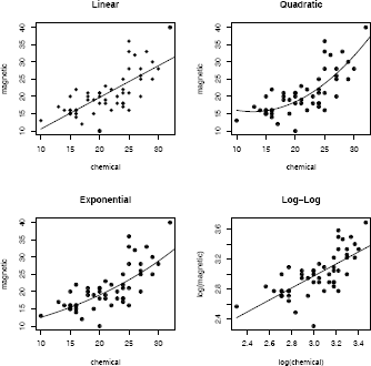
The ironslag (DAAG) data [185] has 53 measurements of iron content by two methods, chemical and magnetic (see “iron.dat” in [126]). A scatterplot of the data in Figure 7.2 suggests that the chemical and magnetic variables are positively correlated, but the relation may not be linear. From the plot, it appears that a quadratic polynomial, or possibly an exponential or logarithmic model might fit the data better than a line.

There are several steps to model selection, but we will focus on the prediction error. The prediction error can be estimated by cross validation, without making strong distributional assumptions about the error variable.

The proposed models for predicting magnetic measurement (Y) from chemical measurement (X) are:

1. Linear: Y = β0 + β1X + ε
2. Quadratic: Y = β0 + β1X+β2 X2+ ε.
3. Exponential: log(Y) = log(ββ0) + β1X + ε.
4. Log-Log: log(Y) = β0 + β0 log(X) + ε.

The code to estimate the parameters of the four models follows. Plots of the predicted response with the data are also constructed for each model and shown in Figure 7.2. To display four plots use par(mfrow=c(2,2)).

  library(DAAG); attach(ironslag)

  a <- seq(10, 40, .1) #sequence for plotting fits

  L1 <- lm(magnetic ~ chemical)

  plot(chemical, magnetic, main="Linear", pch=16)

  yhat1 <- L1$coef[1] + L1$coef[2] * a

  lines(a, yhat1, lwd=2)

  L2 <- lm(magnetic ~ chemical + I(chemical^2))

  plot(chemical, magnetic, main="Quadratic", pch=16)

  yhat2 <- L2$coef[1] + L2$coef[2] * a + L2$coef[3] * a^2

  lines(a, yhat2, lwd=2)

  L3 <- lm(log(magnetic) ~ chemical)

  plot(chemical, magnetic, main="Exponential", pch=16)

  logyhat3 <- L3$coef[1] + L3$coef[2] * a

  yhat3 <- exp(logyhat3)

  lines(a, yhat3, lwd=2)

  L4 <- lm(log(magnetic) ~ log(chemical))

  plot(log(chemical), log(magnetic), main="Log-Log", pch=16)

  logyhat4 <- L4$coef[1] + L4$coef[2] * log(a)

  lines(log(a), logyhat4, lwd=2)

Once the model is estimated, we want to assess the fit. Cross validation can be used to estimate the prediction errors.

Procedure to estimate prediction error by n-fold (leave-one-out) cross validation

1. For k = 1, ... , n, let observation (xk, yk) be the test point and use the remaining observations to fit the model.
   1. Fit the model(s) using only the n − 1 observations in the training set, (xi, yi), i ≠ k.
   2. Compute the predicted response ${\widehat{y}}_k={\widehat{\beta }}_0+{\widehat{\beta }}_1{x}_k$ for the test point.
   3. Compute the prediction error $e_k=y_k-{\widehat{y}}_k.$
2. Estimate the mean of the squared prediction errors ${\widehat{\sigma }}_{\epsilon }^2=\frac{1}{n}{\displaystyle {\sum }_{k=1}^n{e}_k^2.}$

Example 7.18 (Model selection: Cross validation)

Cross validation is applied to select a model in Example 7.17.

  n <- length(magnetic)  #in DAAG ironslag

  e1 <- e2 <- e3 <- e4 <- numeric(n)

  # for n-fold cross validation

  # fit models on leave-one-out samples

  for (k in 1:n) {

  y <- magnetic[-k]

  x <- chemical[-k]

  J1 <- lm(y ~ x)

  yhat1 <- J1$coef[1] + J1$coef[2] * chemical[k]

  e1[k] <- magnetic[k] - yhat1

  J2 <- lm(y ~ x + I(x^2))

  yhat2 <- J2$coef[1] + J2$coef[2] * chemical[k] + 

     J2$coef[3] * chemical[k]^2

  e2[k] <- magnetic[k] - yhat2

  J3 <- lm(log(y) ~ x)

  logyhat3 <- J3$coef[1] + J3$coef[2] * chemical[k]

  yhat3 <- exp(logyhat3)

  e3[k] <- magnetic[k] - yhat3

  J4 <- lm(log(y) ~ log(x))

  logyhat4 <- J4$coef[1] + J4$coef[2] * log(chemical[k])

  yhat4 <- exp(logyhat4)

  e4[k] <- magnetic[k] - yhat4

 }

The following estimates for prediction error are obtained from the n-fold cross validation.

  > c(mean(e1^2), mean(e2^2), mean(e3^2), mean(e4^2))

  [1] 19.55644 17.85248 18.44188 20.45424

According to the prediction error criterion, Model 2, the quadratic model, would be the best fit for the data.

  > L2

  Call: 

  lm(formula = magnetic ~ chemical + I(chemical^2))

  Coefficients:

  (Intercept)  chemical  I(chemical^2)

  24.49262  -1.39334  0.05452

The fitted regression equation for Model 2 is

$\widehat{Y}=24.49262-1.39334X+0.05452X^2.$

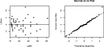
The residual plots for Model 2 are shown in Figure 7.3. An easy way to get several residual plots is by plot(L2). Alternately, similar plots can be displayed as follows.

 par(mfrow = c(2, 2))  #layout for graphs

 plot(L2$fit, L2$res)  #residuals vs fitted values

 abline(0, 0)   #reference line

 qqnorm(L2$res)  #normal probability plot

 qqline(L2$res)  #reference line

 par(mfrow = c(1, 1))  #restore display

Part of the summary for the fitted quadratic model is below.

 Residuals:

 Min  1Q  Median 3Q Max

 -8.4335 -2.7006 -0.2754 2.5446 12.2665

 Residual standard error: 4.098 on 50 degrees of freedom

 Multiple R-Squared: 0.5931, Adjusted R-squared: 0.5768

In the quadratic model the predictors X and X2 are highly correlated. See poly for another approach with orthogonal polynomials.

Exercises

1. 7.1 Compute a jackknife estimate of the bias and the standard error of the correlation statistic in Example 7.2.

2. 7.2 Refer to the law data (bootstrap). Use the jackknife-after-bootstrap method to estimate the standard error of the bootstrap estimate of se(R).

3. 7.3 Obtain a bootstrap t confidence interval estimate for the correlation statistic in Example 7.2 (law data in bootstrap).

4. 7.4 Refer to the air-conditioning data set aircondit provided in the boot package. The 12 observations are the times in hours between failures of air-conditioning equipment [63, Example 1.1]:

   3, 5, 7, 18, 43, 85, 91, 98, 100, 130, 230, 487.

   Assume that the times between failures follow an exponential model Exp(λ). Obtain the MLE of the hazard rate λ and use bootstrap to estimate the bias and standard error of the estimate.

5. 7.5 Refer to Exercise 7.4. Compute 95% bootstrap confidence intervals for the mean time between failures 1/λ by the standard normal, basic, percentile, and BCa methods. Compare the intervals and explain why they may differ.

6. 7.6 Efron and Tibshirani discuss the scor (bootstrap) test score data on 88 students who took examinations in five subjects [84, Table 7.1], [188, Table 1.2.1]. The first two tests (mechanics, vectors) were closed book and the last three tests (algebra, analysis, statistics) were open book. Each row of the data frame is a set of scores (xi1, ... ,xi5)for the ith student. Use a panel display to display the scatter plots for each pair of test scores. Compare the plot with the sample correlation matrix. Obtain bootstrap estimates of the standard errors for each of the following estimates: ${\widehat{\rho }}_{12}=\widehat{\rho }(\text{mec},\text{vec}),{\widehat{\rho }}_{34}=\widehat{\rho }(\text{alg,ana}),{\widehat{\rho }}_{35}=\widehat{\rho }(\text{alg,sta}),{\widehat{\rho }}_{45}=\widehat{\rho }(\text{ana,sta})$.

7. 7.7 Refer to Exercise 7.6. Efron and Tibshirani discuss the following example [84, Ch. 7]. The five-dimensional scores data have a 5 × 5 covariance matrix Σ, with positive eigenvalues λ1 > ... > λ5. In principal components analysis,

   $\theta =\frac{{\lambda }_1}{{\sum }_{j-1}^5{\lambda }_j}$

   measures the proportion of variance explained by the first principal component. Let ${\widehat{\lambda }}_1>\cdots >{\widehat{\lambda }}_5$ be the eigenvalues of $\widehat{\Sigma }$ where $\widehat{\Sigma }$ is the MLE of Σ. Compute the sample estimate

   $\widehat{\theta }=\frac{{\widehat{\lambda }}_1}{{\displaystyle {\sum }_{j=1}^5{\widehat{\lambda }}_j}}$

   of θ. Use bootstrap to estimate the bias and standard error of $\widehat{\theta }$.

8. 7.8 Refer to Exercise 7.7. Obtain the jackknife estimates of bias and standard error of $\widehat{\theta }$.

9. 7.9 Refer to Exercise 7.7. Compute 95% percentile and BCa confidence intervals for $\widehat{\theta }$.

10. 7.10 In Example 7.18, leave-one-out (n-fold) cross validation was used to select the best fitting model. Repeat the analysis replacing the Log-Log model with a cubic polynomial model. Which of the four models is selected by the cross validation procedure? Which model is selected according to maximum adjusted R2?

11. 7.11 In Example 7.18, leave-one-out (n-fold) cross validation was used to select the best fitting model. Use leave-two-out cross validation to compare the models.

Projects

1. 7.A Conduct a Monte Carlo study to estimate the coverage probabilities of the standard normal bootstrap confidence interval, the basic bootstrap confidence interval, and the percentile confidence interval. Sample from a normal population and check the empirical coverage rates for the sample mean. Find the proportion of times that the confidence intervals miss on the left, and the porportion of times that the confidence intervals miss on the right.

2. 7.B Repeat Project 7.A for the sample skewness statistic. Compare the coverage rates for normal populations (skewness 0) and χ2(5) distributions (positive skewness).