
Chapter 11
Numerical Methods in R
11.1 Introduction
This chapter begins with a review of some concepts that should be understood by any statistician who will apply numerical methods that are implemented in statistical packages such as R. Following this introduction, a selection of examples are presented that illustrate the application of numerical methods using functions provided in R. Readers should refer to one or more of the relevant references for a thorough and rigorous presentation of the underlying principles.
Many excellent references are available on numerical methods. Two recent texts written to address the problems of statistical computing in particular are Monahan [202] and Lange [168]. The Monahan text is an excellent resource for statisticians with a limited background in numerical analysis. Nocedal and Wright [206] is a graduate level text on optimization. Lange [169] is another graduate level optimization text that features statistical applications. Thisted [269] covers numerical computation for statistics, including numerical analysis, numerical integration, and smoothing.
Computer representation of real numbers
A positive decimal number x is represented by the ordered coefficients {dj}in the series
dn10n+dn−110n−1+⋯+d1101+d0+d−110−1+d−210−2+⋯
and decimal point separating d0 and d−1, where dj are integers in {0, 1,..., 9}. The same number can be represented in base 2 using the binary digits {0, 1} by akak−1...a1a0.a−1a−2...,where
x=ak2k+ak−12k−1+⋯+a12+a0+a−12−1+a−22−2+⋯,
aj∈{0,1}.The point separating a0 and a−1 is called the radix point. Similarly, x can be represented in any integer base b > 1 by expanding in powers of b.
R note 11.1 The function digitsBase in the package sfsmisc [183] returns the vector of digits that represent a given integer in another base.
Whenever a computer is involved in mathematical calculations, it is very likely to involve the conversions “from” and “to” decimal, because machines and humans represent numbers in different bases. Both types of conversions introduce errors that could be significant in certain cases.
At the lowest level, the computer recognizes exactly two states, like a switch that is on or off, or a circuit that is open or closed. Therefore, at some level, the base 2 representation is used in computer arithmetic. Other powers of 2 such as 8 (octal) or 16 (hexadecimal) are also more natural for low level routines than base 10.
Positive integers can always be represented by a finite sequence of digits, ending with an implicit radix point. For this reason, integers are called fixed point numbers. Numbers that require an explicit radix point in the sequence of digits may be fixed point or floating point (generally treated as floating point in calculations). Floating point numbers are represented by a sign, a finite sequence of digits, and an exponent, similar to the representation of real numbers in scientific notation. In general, this representation of a real number is approximate, not exact.
Even though the internal representation of numbers is usually transparent to the user, who conveniently interacts with the software in the decimal system, it is important in statistical computing to understand that there are fundamental differences between mathematical calculations and computer calculations. Mathematical ideas such as limit, supremum, infimum, etc. cannot be exactly reproduced in the computer. No computer has infinite storage capacity, so only finitely many numbers can be represented in the computer; there is a smallest and a largest positive number. See Monahan [202, Ch. 2] for a discussion of fixed point and floating point arithmetic, and inaccuracies that can occur in algorithms as simple as calculation of sample variance.
R note 11.2 The R variable .Machine holds machine specific constants with information on the largest integer, smallest number, etc. For example, in R-2.5.0 for Windows, the largest integer (.Machine$integer.max) is 231 − 1 = 2147483647. Type .Machine at the command prompt for the complete list. For portability and reusability of code, tolerances or convergence criteria should be given in terms of machine constants. For example, the uniroot function, which seeks a root of a univariate function, has a default tolerance of .Machine$double.eps^0.25.
Occasionally users are surprised to find that some mathematical identities appear to be contradicted by the software. A typical example is
> (.3 - .1)
[1] 0.2
> (.3 - .1) == .2
[1] FALSE
> .2 - (.3 - .1)
[1] 2.775558e-17
The base 2 representation of 0.2 is an infinite series of digits 0.00110011 ..., which cannot be represented exactly in the computer. Notice that although the result above is not exactly equal to 0.2, the error is negligible. Good programming practice avoids testing the equality of two floating point numbers.
Example 11.1 (Identical and nearly equal)
R provides the function all.equal to check for near equality of two R objects. In a logical expression, use isTRUE to obtain a logical value.
> isTRUE(all.equal(.2, .3 - .1))
[1] TRUE
> all.equal(.2, .3) #not a logical value
[1] "Mean relative difference: 0.5"
> isTRUE(all.equal(.2, .3)) #always a logical value
[1] FALSE
The isTRUE function is applied in Example 11.9. The identical function is available for testing whether two objects are identical. The help topic for identical gives very clear and explicit advice to programmers: “A call to identical is the way to test exact equality in if and while statements, as well as in logical expressions that use && or ||. In all these applications you need to be assured of getting a single logical value.” Also see the examples below.
> x <- 1:4
> y <- 2
> y == 2
[1] TRUE
> x == y #not necessarily a single logical value
[1] FALSE TRUE FALSE FALSE
> identical(x, y) #always a single logical value
[1] FALSE
> identical(y, 2)
[1] TRUE
Overflow occurs when the result of an arithmetic operation exceeds the maximum floating point number that can be represented. Underflow occurs when the result is smaller than the minimum floating point number. In the case of underflow, the result might unexpectedly be returned as zero. This could lead to division by zero or other problems that produce unexpected and possibly inaccurate results – without warning. Overflow is usually more obvious, but should be avoided. Good algorithms should set underflows to zero and give a warning if this may produce unexpected results. Programmers can avoid many of these problems, however, by carefully coding arithmetic expressions with the limitations of the machine in mind.
Often the expression to be evaluated is not impossible to compute, but one needs to be careful about the order of operations. One of the most common, and easily avoided problems occurs when we need to compute a ratio of two very large or very small numbers. For example, n!/(n−2)!=n(n−1),but we could easily have trouble computing the numerator or denominator if n is large. A good approach for this type of problem is to take the logarithm of the quotient and exponentiate the result. A typical example that arises in statistical applications is the following.
Example 11.2 (Ratio of two large numbers)
Evaluate
Γ((n−1)/2)Γ(1/2)Γ((n−2)/2)
This could be coded using the gamma function in R, but Γ(n) = (n − 1)!, so when n is large, gamma may return Inf and the arithmetic operations could return NaN. On the other hand, although numerator and denominator are both large, the ratio is much smaller. Compute the ratio Γ((n − 1)/2)/Γ((n − 2)/2) using the logarithm of the gamma function lgamma. That is, Γ(n)/Γ(m) = exp(lgamma(n) - lgamma(m)). Also, recall that Γ(1/2)=√π.
> n <- 400
> (gamma((n-1)/2) / (sqrt(pi) * gamma((n-2)/2)))
[1] NaN
> exp(lgamma((n-1)/2) - lgamma((n-2)/2)) / sqrt(pi)
[1] 7.953876
A thorough discussion of computer arithmetic is beyond the scope of this text. Among the references, Monahan [202] or Thisted [269] are good starting points on this topic for statistical computing; on computer arithmetic and algorithms see e.g. Higham [142] or Knuth [164].
Evaluating Functions
The power series expansion of a function is commonly applied. If f(x) is analytic, then f(x) can be evaluated in a neighborhood of the point x0 by a power series
f(x)=∞∑k=0ak(x−x0)k.
The Taylor series representation of f(x) in a neighborhood of x0 is
f(x)=∞∑k=0f(k)(x0)k!(x−x0)k,
also called a Maclaurin series when x0 = 0. The infinite series must be truncated in order to obtain a numerical approximation. The power series approximation is thus a (high degree) polynomial approximation. If f has continuous derivatives up to order (n + 1) in a neighborhood of 0, then the finite Taylor expansion of f(x) at x0 = 0 is
limx→0f(x)=n∑k=0f(k)(0)k!xk+Rn(x),
where Rn(x)=O(xn+1).
Recall that “O“ (big oh) and “o“ (little oh) describe the order of convergence of functions. Let f and g be defined on a common interval (a, b) and let a ≤ x0 ≤ b. Suppose that g(x) ≠ 0 for all x ≠ x0 in a neighborhood of x0. Then f(x) = O(g(x)) if there exists a constant M such that |f(x)| ≤ M|g(x)| as x → x0. If limx→x0 f(x)/g(x) = 0 then f(x) = o(g(x)).
If the finite Taylor expansion is computed in a language such as C or fortran, a method is used that avoids repeated multiplications. That is, if yk = xk/k! then
1k!f(k)(0)xk=ykf(k)(0)=yk−1(x/k)f(k)(0),
saving many multiplications. Computing in R, however, it will usually be faster to take advantage of the vectorized operations, provided it is known how many terms are required.
Example 11.3 (Taylor expansion)
Consider the finite Taylor expansion for the sine function,
sinx=n∑k=0(−1)k(2k+1)!x2k+1.
For example, evaluate sin(π/6) from the Taylor polynomial.
The remainder term Rn(x) = O(xn+1) can be used to determine the approximate number of terms required in the finite expansion. Suppose that a 24th degree polynomial is sufficiently accurate at x = π/6. Two methods of computing the Taylor polynomial are compared below.
The following method of calculation is efficient in C or fortran code, but not in R. The timer measures 1000 calculations of the Taylor polynomial.
system.time({
for (i in 1:1000) {
a <- rep(0, 24)
a0 <- pi / 6
a2 <- a0 * a0
a[1] <- -a0^3 / 6
for (i in 2:24)
a[i] <- - a2 * a[i-1] / ((2*i+1)*(2*i))
a0 + sum(a)}
})
[1] 0.36 0.01 0.49 NA NA
Compare the version above to the vectorized version below. The vectorized version appears to be about 5 times faster than the method above. In R code, vectorized operations like the code below are usually more efficient than loops.
system.time({
for (i in 1:1000) {
K <- 2 * (0:24) + 1
i <- rep(c(1, -1), length=25)
sum(i * (pi/6)^K / factorial(K))}
})
[1] 0.07 0.01 0.08 NA NA
Power series expansions are also useful for numerical evaluation of derivatives. Within the common region of the radius of convergence of the power series and its derivative, one can differentiate the finite expansion term by term. The next example illustrates this method with a useful function for the derivative of the zeta function.
Example 11.4 (Derivative of zeta function)
The Riemann zeta function is defined by
ζ(a)=∞∑i=11ia,
which converges for all a > 1. Write a function to evaluate the first derivative of the zeta function.
It can be shown that
ζ(a)=1z−1+∞∑n=0(−1)nn!γn(z−1)n,
γn=ζ(n)(z)−(−1)nn!(z−1)n+1|z=1=limm→∞[m∑k=1(logk)nk−(logm)n+1n+1]
are the Stieltjes constants. Differentiating ζ(a) gives
ζ′(a)=−1(z−1)2−γ1+γ2(z−1)−12γ3(z−1)2+⋯, a>1.
The Stieltjes constants can be evaluated numerically, and tables of the Stieltjes constants are available [1]. More terms can be added if greater accuracy is needed, but to conserve space, only five of the constants are used in the version below. This “light” version of the zeta derivative gives remarkably good results over the interval (1, 2) (see the next example).
zeta.deriv <- function(a) {
z <- a - 1
# Stieltjes constants gamma_k for k=1:5
g <- c(
-.7281584548367672e-1,
-.9690363192872318e-2,
.2053834420303346e-2,
.2325370065467300e-2,
.7933238173010627e-3)
i <- c(-1, 1, -1, 1, -1)
n <- 0:4
-1/z^2 + sum(i * g * z^n / factorial(n))
}
Another approach to numerical evaluation of the derivative of a function applies the following central difference formula
f′(x) ≈_f(x+h)−f(x−h)2h,
for a small value of h. According to [213], h should be chosen so that x and x + h differ by an exactly representable number.
Example 11.5 (Derivative of zeta function, cont.)
Compare the finite series approximation of the numerical derivative in Example 11.4 with the central difference formula. That is, for small h, compare
ζ(a+h)−ζ(a−h)2h
with the value returned by zeta.deriv(a) in Example 11.4. The ζ(·) function is implemented in the GNU scientific library, available in the gsl package [127].
library(gsl) #for zeta function
z <- c(1.001, 1.01, 1.5, 2, 3, 5)
h <- .Machine$double.eps^0.5
dz <- dq <- rep(0, length(z))
for (i in 1:length(z)) {
v <- z[i] + h
h <- v - z[i]
a0 <- z[i] - h
if (a0 < 1) a0 <- (1 + z[i])/2
a1 <- z[i] + h
dq[i] <- (zeta(a1) - zeta(a0)) / (a1 - a0)
dz[i] <- zeta.deriv(z[i])
}
h
[1] 1.490116e-08
cbind(z, dz, dq)
z dz dq
[1,] 1.001 -9.999999e+05 -9.999999e+05
[2,] 1.010 -9.999927e+03 -9.999927e+03
[3,] 1.500 -3.932240e+00 -3.932240e+00
[4,] 2.000 -9.375469e-01 -9.375482e-01
[5,] 3.000 -1.981009e-01 -1.981262e-01
[6,] 5.000 -2.853446e-02 -2.857378e-02
Values of z are given in the first column, values of ζ′(z) computed by the finite series approximation are given in column dz, and values of ζ′(z) computed by the central difference formula are given in column dq. Although the two estimates are quite close, it appears that the difference in the two estimates is increasing with z. The finite series approximation can be improved by adding more terms.
11.2 Root-finding in One Dimension
This section will briefly summarize the main ideas behind the Brent minimization algorithm [32], on which the R root-finding function uniroot is based, and illustrate its application with examples. Refer to [32, 169, 213, 206] for more details. The source code of the fortran implementation “zeroin.f” in the GNU Scientific Library (GSL) can be found at the web site http://www.gnu.org/software/gsl/.
Let f(x) be a continuous function f:ℝ1→ℝ1. A root (or zero) of the equation f(x) = c is a number x such that g(x) = f(x) − c = 0. Thus, we can restrict attention to solving f(x) = 0.
One can choose from numerical methods that require evaluation of the first derivative of f(x), and algorithms that do not require the first derivative. Newtons’s method or Newton-Raphson method are examples of the first type, while Brent’s algorithm is an example of the second type of method. In either case, one must bracket the root between two endpoints where f(·) has opposite signs.
Bisection method
If f(x) is continuous on [a, b], and f(a), f(b) have opposite signs, then by the intermediate value theorem it follows that f(c) = 0 for some a < c < b. The bisection method simply checks the sign of f(x) at the midpoint x = (a+b)/2 of the interval at each iteration. If f(a), f(x) have opposite signs, then the interval is replaced by [a, x] and otherwise it is replaced by [x, b]. At each iteration, the length of the interval containing the root decreases by half. The method cannot fail, and the number of iterations needed to achieve a specified tolerance is known in advance. If the initial interval [a, b] contains more than one root, then bisection will find one of the roots. The rate of convergence of the bisection algorithm is linear.
Example 11.6 (Solving f(x) = 0)
Solve
a2+y2+2ayn−1=n−2,
where a is a specified constant and n > 2 is an integer. Of course, this equation can be solved directly by elementary algebra, to obtain the exact solution:
y=−an−1±√n−2+a2+(an−1)2.
Let us compare the exact solution with a numerical solution. Apply the bisection method to seek a positive solution. If we restate the problem as: find the solutions of
f(y)=a2+y2+2ayn−1−(n−1)=0,
the first step is to code the function f. The next step is to determine an interval such that f(y) has opposite signs at the endpoints. For example, if a = 1/2 and n = 20, there will be a positive and a negative root. In the following, the positive root is found, starting from the interval (0, 5n).
f <- function(y, a, n) {
a^2 + y^2 + 2*a*y/(n-1) - (n-2)
}
a <- 0.5
n <- 20
b0 <- 0
b1 <- 5*n
#solve using bisection
it <- 0
eps <- .Machine$double.eps^0.25
r <- seq(b0, b1, length=3)
y <- c(f(r[1], a, n), f(r[2], a, n), f(r[3], a, n))
if (y[1] * y[3] > 0)
stop("f does not have opposite sign at endpoints")
while(it < 1000 && abs(y[2]) > eps) {
it <- it + 1
if (y[1]*y[2] < 0) {
r[3] <- r[2]
y[3] <- y[2]
} else {
r[1] <- r[2]
y[1] <- y[2]
}
r[2] <- (r[1] + r[3]) / 2
y[2] <- f(r[2], a=a, n=n)
print(c(r[1], y[1], y[3]-y[2]))
}
The estimate of the root when the stopping condition is satisfied is the value in r[2] and the value of the function at r[2] is in y[2].
> r[2]
[1] 4.186845
> y[2]
[1] 2.984885e-05
> it
[1] 21
Our exact formula gives the roots y = 4.186841, −4.239473. (Most problems, including this one, can be solved more efficiently using the uniroot function, which is shown in Example 11.7 below.)
Other methods, such as the secant method, may (formally) converge faster than the bisection method, but the root may not remain bracketed. These superlinear methods may be faster for many problems, but may fail to converge to a root. The secant method assumes that f(x) is approximately linear on the interval bracketing the root. Inverse quadratic interpolation approximates f(x) with a quadratic function fitted to the three prior points.
Brent’s method
Brent’s method combines the root bracketing and bisection with inverse quadratic interpolation. It fits x as a quadratic function of y. If the three points are (a, f(a)), (b, f(b)), (c, f(c)), with b as the current best estimate, the next estimate for the root is found by interpolation, setting y = 0 in the Lagrange interpolation polynomial
x=[y−f(a)][y−f(b)]c[f(c)−f(a)][f(c)−f(b)] +[y−f(a)][y−f(c)]a[f(a)−f(b)][f(a)−f(c)]+[y−f(c)][y−f(a)]b[f(b)−f(c)][f(b)−f(a)].
If this estimate is outside of the interval known to bracket the root, bisection is used at this step. (For details see [32] or[213] or the zeroin.f fortran code.) Brent’s method is generally faster than bisection, and it has the sure convergence of the bisection method.
Brent’s method is implemented in the R function uniroot, which searches for a zero of a univariate function between two points where the function has opposite signs.
Example 11.7 (Solving f(x) = 0 with Brent’s method: uniroot)
Solve
a2+y2+2ayn−1=n−2,
with a = 0.5, n = 20 as in Example 11.6. The first step is to code the function f. This function is not complicated, so we code this function inline in the uniroot statement. The next step is to determine an interval such that f(y) has opposite signs at the endpoints. The call to uniroot and result are shown below.
a <- 0.5
n <- 20
out <- uniroot(function(y) {
a^2 + y^2 + 2*a*y/(n-1) - (n-2)},
lower = 0, upper = n*5)
> unlist(out)
root f.root iter estim.prec
4.186870e+00 2.381408e-04 1.400000e+01 6.103516e-05
In the call to uniroot, we can optionally specify the maximum number of iterations (default 1000) or the tolerance (default .Machine$double.eps^0.25). The positive solution to f(y) = 0 is (approximately) y = 4.186870. To seek the negative root, we can apply uniroot again. The interval can be specified as above, or as shown below.
uniroot(function(y) {a^2 + y^2 + 2*a*y/(n-1) - (n-2)},
interval = c(-n*5, 0))$root
[1] -4.239501
Our exact formula (see Example 11.6) gives y = 4.186841, −4.239473.
R note 11.3 Also see the polyroot function, to find zeroes of a polynomial with real or complex coefficients. See the help topic Complex for description of functions in R that support complex arithmetic.
11.3 Numerical Integration
Basic numerical integration using the integrate function is illustrated in the following examples, where useful functions are developed for the density and cdf of the sample correlation statistic.
Numerical integration methods can be adaptive or non-adaptive. Non-adaptive methods apply the same rules over the entire range of integration. The integrand is evaluated at a finite set of points and a weighted sum of these function values is used to obtain the estimate. The numerical estimate of ∫baf(x) is of the form ∑ni=0f(xi)wi, where {xi} are points in an interval containing [a, b] and {wi} are suitable weights.
For example, the trapezoidal rule divides [a, b] into n equal length subintervals length h = (b − a)/n, with endpoints x0, x1, ... , xn, and uses the area of the trapezoid to estimate the integral over each subinterval. The estimate on (xi, xi+1) is (f(xi) + f(xi+1))(h/2). The numerical estimate of ∫baf(x)dxis
h2f(a)+hn−1∑i=1f(xi)+h2f(b).
If f(x) is twice continuously differentiable, the error is O(f”(x*)/n2), where x* ∈ (a, b). This is an example of a closed Newton-Cotes integration formula. See e.g. [269, Ch. 5] for more examples.
Quadrature methods evaluate the integrand at a finite set of points (nodes), but these nodes need not be evenly spaced. Suppose that w is a non-negative function such that ∫baxkw(x)dx<∞, for all k ≥ 0. Then the integrand f(x) can be expressed as g(x)w(x).
Note that we have assumed that w(x)/∫baw(x)dx is a density function with finite positive moments. For example, we can take w(x) = exp (−x2/2), called Gauss-Hermite quadrature. In this case,∫∞−∞xkw(x)dx<∞, for all k ≥ 0, which applies to arbitrary intervals (a, b) on the real line. In Gaussian quadrature, the nodes {xi} selected are the roots of a set of orthogonal polynomials with respect to {wi}. The normalized orthogonal polynomials also determine weights {wi}.
The Gaussian Quadrature Theorem implies that if g(x) is 2n times continuously differentiable, then the error in the numerical estimate ∑ni=1wig(xi)is
∫bag(x)w(x)dx−n∑i=1wig(xi)=g(2n)(x*)(2n)!k2n,
where kn is the leading coefficient of the nth polynomial and x* ∈ (a, b). Quadrature and other approaches to numerical integration are discussed in more detail in [121, 168, 269].
When an integrand behaves well in one part of the range of integration, but not so well in another part, it helps to treat each part differently. Adaptive methods choose the subintervals based on the local behavior of the integrand.
The integrate function provided in R uses an adaptive quadrature method to find the approximate value of the integral of a one variable function. The limits of integration can be infinite. The maximum number of subintervals, the relative error and the absolute error can be specified, but have reasonable default values for many problems.
Example 11.8 (Numerical integration with integrate)
Compute
∫∞0dy(coshy−pr)n−1, (11.1)
where −1< ρ < 1, −1< r < 1 are constants and n ≥ 2 is an integer. The graph of the integrand is shown in Figure 11.1(a). We apply adaptive quadrature implemented by the integrate function provided in R.
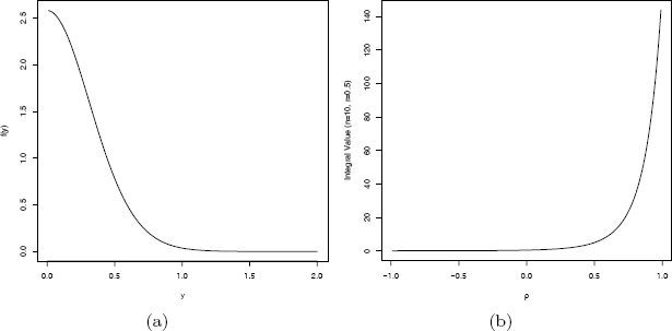
Example 11.8 (n = 10, r = 0.5, ρ = 0.2) (a) Integrand, (b) Value of the integral as a function of ρ.
First write a function that returns the value of the integrand. This function should take as its first argument a vector containing the nodes, and return a vector of the same length. Additional arguments can also be supplied. This function or the name of this function is the first argument to integrate.
A simple way to compute the integral for fixed parameters, say (n = 10, r = 0.5, ρ = 0.2) is
> integrate(function(y){(cosh(y) - 0.1)^(-9)}, 0, Inf)
1.053305 with absolute error < 2.3e-05
The integral for arbitrary (n, r, ρ) is needed, so write a more general integrand function with these arguments, and supply the extra arguments in the call to integrate.
f <- function(y, N, r, rho) {
(cosh(y) - rho * r)^(1 - N)
}
integrate(f, lower=0, upper=Inf,
rel.tol=.Machine$double.eps^0.25,
N=10, r=0.5, rho=0.2)
This version produces the same estimate as above.
To see how the result depends on ρ, fix n = 10 and r = 0.5 and plot the value of the integral as a function of ρ. The plot is shown in Figure 11.1(b), as produced by the following code.
ro <- seq(-.99, .99, .01)
v <- rep(0, length(ro))
for (i in 1:length(ro)) {
v[i] <- integrate(f, lower=0, upper=Inf,
rel.tol=.Machine$double.eps^0.25,
N=10, r=0.5, rho=ro[i])$value
}
plot(ro, v, type="l", xlab=expression(rho),
ylab="Integral Value (n=10, r=0.5)")
R note 11.4 Sometimes there is a conflict between named arguments and optional user-supplied arguments. To avoid the conflict, either choose another name for the optional argument, or supply both arguments. For example, the following produces an error, because of apparent ambiguity between argument rel.tol and R.
> integrate(f, lower=0, upper=Inf, n=10, r=0.5, rho=0.2)
Error in f(x, ...) : argument "r" is missing, with no default
The integral (11.1) appears in a density function in the following example.
Example 11.9 (Density of sample correlation coefficient)
The sample product-moment correlation coefficient measures linear association between two variables. The population correlation coefficient of (X, Y) is
ρ=E[(X−E(X))(Y−E(Y))]√Var(X)Var(Y).
If {(Xj, Yj), j = 1, ... , n} are paired sample observations, the sample correlation coefficient is
R=∑nj=1(Xj−ˉX)(Yj−ˉY)[∑nj=1(Xj−ˉX)2∑nj=1(Yj−ˉY)2]1/2.
Assume that {(Xj, Yj), j = 1, ... , n} are iid with BV N(µ1, µ2, σ1, σ2, ρ) (bivariate normal) distribution. If ρ = 0, the density function of R (see e.g. [157, Ch. 32]) is given by
f(r)=Γ((n−1)/2)Γ(1/2)Γ((n−2)/2)(1−r2)(n−4)/2, −1<r<1. (11.2)
For 0 < |ρ| < 1, the density function is more complicated. Several forms of the density function are given in [157, p. 549], including:
f(r)=(n−1)(1−ρ2)(n−1)/2(1−r2)n−4/2π∫∞0dw(coshw−ρr)n−1, (11.3)
for −1< r< 1.
To evaluate the density function (11.3), the integral must be evaluated. This is covered in Example 11.8. The case ρ = 0 can be handled separately using the simpler formula (11.2). The method for evaluating the constant Γ((n − 1)/2)/Γ((n − 2)/2) was discussed in Example 11.2. The following function combines these results to evaluate the density of the correlation statistic.
.dcorr <- function(r, N, rho=0) {
# compute the density function of sample correlation
if (abs(r) > 1 || abs(rho) > 1) return (0)
if (N < 4) return (NA)
if (isTRUE(all.equal(rho, 0.0))) {
a <- exp(lgamma((N - 1)/2) - lgamma((N - 2)/2)) /
sqrt(pi)
return (a * (1 - r^2)^((N - 4)/2))
}
# if rho not 0, need to integrate
f <- function(w, R, N, rho)
(cosh(w) - rho * R)^(1 - N)
#need to insert some error checking here
i <- integrate(f, lower=0, upper=Inf,
R=r, N=N, rho=rho)$value
c1 <- (N - 2) * (1 - rho^2)^((N - 1)/2)
c2 <- (1 - r^2)^((N - 4) / 2) / pi
return(c1 * c2 * i)
}
Some error checking should be added to this function in case the numerical integration fails.
As an informal check on the density calculations, plot the density curve. For ρ = 0 the density curve should be symmetric about 0 and the shape should resemble a symmetric beta density. The plot is shown in Figure 11.2.
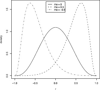
r <- as.matrix(seq(-1, 1, .01))
d1 <- apply(r, 1, .dcorr, N=10, rho=.0)
d2 <- apply(r, 1, .dcorr, N=10, rho=.5)
d3 <- apply(r, 1, .dcorr, N=10, rho=-.5)
plot(r, d2, type="l", lty=2, lwd=2, ylab="density")
lines(r, d1, lwd=2)
lines(r, d3, lty=4, lwd=2)
legend("top", inset=.02, c("rho = 0", "rho = 0.5",
"rho = -0.5"), lty=c(1,2,4), lwd=2)
R note 11.5 Density functions in R are vectorized, but the function .dcorr of Example 11.3 is really expecting a single number r, rather than a vector. Later this function can be extended to a general version dcorr, like the density functions dnorm, dgamma, etc. in R that accept vector arguments.
11.4 Maximum Likelihood Problems
Maximum likelihood is a method of estimation of parameters of a distribution. The abbreviation MLE may refer to maximum likelihood estimation (the method), to the estimate, or to the estimator. The method finds a value of the parameter that maximizes the likelihood function. Thus, an important class of optimization problems in statistics are maximum likelihood problems.
Suppose that X1, ... , Xn are random variables with parameter θ ∈ Θ(θ may be a vector). The likelihood function L(θ) of random variables X1, ... , Xn evaluated at x1, ... , xn is defined as the joint density
L(θ) = f(x1, ... , xn; θ).
If X1, ... , Xn are a random sample (so X1, ... , Xn are iid) with density f(x; θ), then
L(θ)=n∏i=1f(xi;θ).
A maximum likelihood estimate of θ is a value ˆθthat maximizes L(θ). That is, ˆθis a solution (not necessarily unique) to
L(ˆθ)=f(x1,...,xn;ˆθ)=mθa∈xΘ f(x1,...,xn;θ). (11.4)
If ˆθ. is unique, ˆθis the maximum likelihood estimator (MLE) of θ.
If θ is a scalar, the parameter space Θ is an open interval, and L(θ) is differentiable and assumes a maximum on Θ, then ˆθis a solution of
ddθL(θ)=0. (11.5)
The solutions to (11.5) are solutions to
ddθl(θ)=0, (11.6)
where l(θ)=logL(θ) is the log-likelihood. In the case where X1, ... , Xn are a random sample, we have
l(θ)=n∏i=1f(xi;θ)=n∑i=1logf(xi;θ),
so (11.6) is often easier to solve than (11.5).
Example 11.10 (MLE using mle)
Suppose Y1, Y2 are iid with density f(y) = θe−θy, y > 0. Find the MLE of θ. By independence,
L(θ)=(θe−θy1)(θe−θy2)=θ2e−θ(y1+y2).and the log-likelihood equation to be solved is
ddθl(θ)=2θ−(y1+y2)=0, θ>0.
The unique solution is ˆθ=2/(y1+y2), which maximizes L(θ). Therefore the MLE is the reciprocal of the sample mean in this example.
Although we have the analytical solution, let us see how the problem can be solved numerically using the mle (stats4) function. The mle function takes as its first argument the function that evaluates −ℓ(θ) = − log(L(θ)). The negative log-likelihood is minimized by a call to optim, an optimization routine.
#the observed sample
y <- c(0.04304550, 0.50263474)
mlogL <- function(theta=1) {
#minus log-likelihood of exp. density, rate 1/theta
return(- (length(y) * log(theta) - theta * sum(y)))
}
library(stats4)
fit <- mle(mlogL)
summary(fit)
Maximum likelihood estimation
Call: mle(minuslogl = mlogL)
Coefficients:
Estimate Std. Error
theta 3.66515 2.591652
-2 log L: -1.195477
Alternately, the initial value for the optimizer could be supplied in the call to mle; two examples are
mle(mlogL, start=list(theta=1))
mle(mlogL, start=list(theta=mean(y)))
In this example, the maximum likelihood estimate is ˆθ=1/ˉY=3.66515. The maximum log-likelihood is l(ˆθ)=2log(1/ˉy)−(1/ˉy)(y1+y2)=0.5977386, or −2 log(L) = −1.195477. The same result was obtained by mle.
Suppose ˆθsatisfies (11.6). Then ˆθmay be a relative maximum, relative minimum, or an inflection point of ℓ(θ). If ℓ″(ˆθ)<0,then ˆθis a local maximum of log ℓ(θ).
The second derivative of the log-likelihood also contains information about the variance of ˆθ. The Fisher information (see e.g. [39, 231]) on X at θ is defined
ℐ(θ)=[−Eθℓ″(θ)]|θ.
The Fisher information gives a bound on the variance of unbiased estimators of θ. The larger the information ℐ(θ), the more information the sample contains about the value of θ, and the smaller the variance of the best unbiased estimator.
If θ is a vector in ℝd,Θ is an open subset of ℝd, and the first order partial derivatives of L(θ) exist in all coordinates of θ, then ˆθmust satisfy simultaneously the d equations
∂∂θjL(ˆθ)=0, j=1,...,d, (11.7)
or the d corresponding log-likelihood equations.
If the log-likelihood is not quadratic, the solution of the likelihood equations (11.11) is a nonlinear system of d equations in d variables. Thus, maximum likelihood estimation and maximum likelihood based inference often require nonlinear numerical methods.
Note that there are several potential problems to finding a solution: the derivatives of the likelihood function may not exist, or may not exist on all of Θ; the optimal θ may not be an interior point of Θ; or the likelihood equation (11.5) or (11.7) may be difficult to solve. In this case, numerical methods of optimization may succeed in finding optimal solutions ˆθsatisfying (11.4).
11.5 One-dimensional Optimization
There are several approaches to one-dimensional optimization implemented in R. Many types of problems can be restated so that the root-finding function uniroot can be applied. The nlm function implements nonlinear minimization with a Newton-type algorithm. The documentation for the optimize function indicates that it is C translation of Fortran code based on the Algol 60 procedure “localmin” given in [32], which implements a combination of golden section search and successive parabolic interpolation.
Example 11.11 (One-dimensional optimization with optimize)
Maximize the function
f(x)=log(1+log(x))log(1+x)
with respect to x. The graph of f(x) in Figure 11.3 shows that the maximum occurs between 4 and 8.
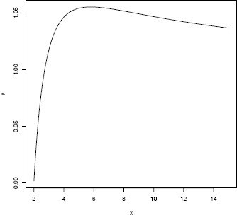
x <- seq(2, 8, .001)
y <- log(x + log(x))/(log(1+x))
plot(x, y, type = "l")
Apply optimize on the interval (4, 8). The default is to minimize the function. To maximize f(x), set maximum = TRUE. The default tolerance is .Machine$double.eps^0.25.
f <- function(x)
log(x + log(x))/log(1+x)
> optimize(f, lower = 4, upper = 8, maximum = TRUE)
$maximum
[1] 5.792299
$objective
[1] 1.055122
Example 11.12 (MLE: Gamma distribution)
Let x1, ... , xn be a random sample from a Gamma(r, λ) distribution (r is the shape parameter and λ is the rate parameter). In this example, θ=(r,λ)∈ℝ2 and Θ=ℝ+×ℝ+. Find the maximum likelihood estimator of θ = (r, λ).
The likelihood function is
L(r,λ)=λnrΓ(r)nn∏i=1xr−1iexp (−λn∑i=1xi), xi≥0,
and the log-likelihood function is
l(r,λ)=nrlogλ−nlogΓ(r)+(r−1)n∑i=1logxi−λn∑i=1xi. (11.8)
The problem is to maximize (11.8) with respect to r and λ. In this form it is a two-dimensional optimization problem. This problem can be reduced to a one-dimensional root-finding problem. Find the simultaneous solution(s) (r, λ) to
∂∂λℓ(r,λ)=nrλ−n∑i=1xi=0;(11.9)
∂∂λℓ(r,λ)=nlogλ−nΓ′(r)Γ(r)+n∑i=1logxi=0.(11.10)
Equation (11.9) implies ˆλ=ˆr/ˉx Substituting ˆλfor λ in (11.10) reduces the problem to solving
nlogˆrˉx+∑ni=1logxi−nΓ′(ˆr)Γ(ˆr)=0 (11.11)
for ˆr. Thus, the MLE (ˆr,ˆλ)is the simultaneous solution (r, λ) of
logλ+1n∑ni=1logxi=ψ(λˉx); ˉx=rλ,
where ψ(t)=ddtlogΓ(t)/Γ′(t)/Γ(t) (the digamma function in R). A numerical solution is easily obtained using the uniroot function.
In the following simulation experiment, random samples of size n = 200 are generated from a Gamma(r = 5, λ = 2) distribution, and the parameters are estimated by optimizing the likelihood equations using uniroot. The sampling and estimation is repeated 20000 times. Below is a summary of the estimates obtained by this method.
m <- 20000
est <- matrix(0, m, 2)
n <- 200
r <- 5
lambda <- 2
obj <- function(lambda, xbar, logx.bar) {
digamma(lambda * xbar) - logx.bar - log(lambda)
}
for (i in 1:m) {
x <- rgamma(n, shape=r, rate=lambda)
xbar <- mean(x)
u <- uniroot(obj, lower = .001, upper = 10e5,
xbar = xbar, logx.bar = mean(log(x)))
lambda.hat <- u$root
r.hat <- xbar * lambda.hat
est[i,] <- c(r.hat, lambda.hat)
}
ML <- colMeans(est)
[1] 5.068116 2.029766
The average estimate for the shape parameter r was 5.068116 and the average estimate for λ was 2.029766. The estimates are positively biased, but close to the target parameters (r = 5, λ = 2).
Recall that a maximum likelihood estimator is asymptotically normal. For large n, ˆλ~N(λ,σ21)and ˆr~N(r,σ22)where σ21 and σ22 are the Cramér-Rao lower bounds of λ and r, respectively. The histogram of replicates ˆλis shown in Figure 11.4(a), and the histogram of replicates ˆris shown in Figure 11.4(b). Here n = 200 is not very large, and the histogram of replicates in both cases is slightly skewed but close to normal.
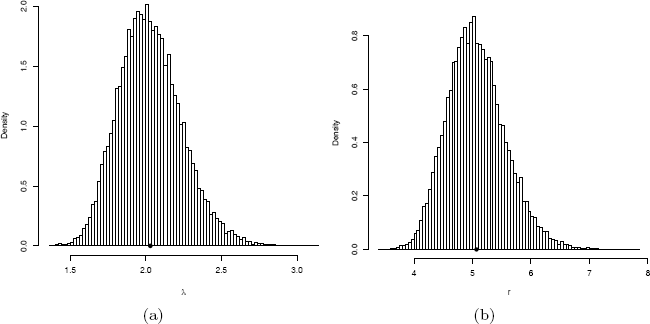
Replicates of maximum likelihood estimates by numerical optimization of the likelihood of a Gamma(r = 5, λ = 2) random variable in Example 11.12.
hist(est[, 1], breaks="scott", freq=FALSE,
xlab="r", main="")
points(ML[1], 0, cex=1.5, pch=20)
hist(est[, 2], breaks="scott", freq=FALSE,
xlab=bquote(lambda), main="")
points(ML[2], 0, cex=1.5, pch=20)
11.6 Two-dimensional Optimization
In the gamma MLE problem we seek the maximum of a two parameter likelihood function. Although it is possible to simplify the problem and solve it as in Example 11.12, it serves as a simple example to illustrate the optim general purpose optimization function in R. It implements Nelder-Mead [205], quasi-Newton, and conjugate-gradient algorithms [96], and also methods for box-constrained optimization and simulated annealing. See Nocedal and Wright [206] and the R manual [217] for reference on these methods and their implementation. The syntax for optim is
optim(par, fn, gr = NULL, method =
c("Nelder-Mead", "BFGS", "CG", "L-BFGS-B", "SANN"),
lower = -Inf, upper = Inf,
control = list(), hessian = FALSE, ...)
The default method is Nelder-Mead. The first argument par is a vector of initial values of the target parameters, and fn is the objective function. The first argument to fn is the vector of target parameters and its return value should be a scalar.
Example 11.13 (Two-dimensional optimization with optim)
The objective function to be maximized is the log-likelihood function
logL(θ|x)=nrlogλ+(r−1)∑ni=1logxi−λ∑ni=1xi−nlogΓ(r),
and the parameters are θ = (r, λ). The log-likelihood function is implemented as
LL <- function(theta, sx, slogx, n) {
r <- theta[1]
lambda <- theta[2]
loglik <- n * r * log(lambda) + (r - 1) * slogx -
lambda * sx - n * log(gamma(r))
- loglik
}
which avoids some repeated calculation of the sums sx=∑ni=1xi and slogx=∑ni=1logxi. As optim performs minimization by default, the return value is − log L(θ). Initial values for the estimates must be chosen carefully. For this problem, the method of moments estimators could be given for the initial values of the parameters, but for simplicity r = 1 and λ = 1 are used here as the initial values. If x is the random sample of size n, the optim call is
optim(c(1,1), LL, sx=sum(x), slogx=sum(log(x)), n=n)
The return object includes an error code $convergence, which is 0 for success and otherwise indicates a problem. The MLE is computed for one sample below.
n <- 200
r <- 5; lambda <- 2
x <- rgamma(n, shape=r, rate=lambda)
optim(c(1,1), LL, sx=sum(x), slogx=sum(log(x)), n=n)
# results from optim
par1 5.278565
par2 2.142059
value 284.550086
counts.function 73.000000
counts.gradient NA
convergence 0.000000
This result indicates that the Nelder-Mead (default) method successfully converged to ˆr=5.278565and ˆλ=2.142059. The precision can be adjusted by reltol. The algorithm stops if it is unable to reduce the value by a factor of reltol, which defaults to sqrt(.Machine$double.eps) = 1.490116e-08 in this computation.
The simulation experiment below repeats the estimation procedure for comparison with the results in Example 11.12.
mlests <- replicate(20000, expr = {
x <- rgamma(200, shape = 5, rate = 2)
optim(c(1,1), LL, sx=sum(x), slogx=sum(log(x)), n=n)$par
})
colMeans(t(mlests))
[1] 5.068109 2.029763
The estimates obtained by the two-dimensional optimization of (11.8) have approximately the same average value as the estimates obtained by the one-dimensional root-finding approach in Example 11.12.
R note 11.6 When replicating a vector, note that replicate fills a matrix in column major order. In the example above, the vector in each replicate is length 2, so the matrix has 2 rows and 20000 columns. The transpose of this result is the two dimensional sample of replicates.
Example 11.14 (MLE for a quadratic form)
Consider the problem of estimating the parameters of a quadratic form of centered Gaussian random variables given by
Y=λ1X21+λ2X22+...+λkX2k,
where Xj are iid standard normal random variables, j = 1, ... , k, and λ1 >· · ·> λk > 0. By elementary transformations, each Yj=λjX2j has a gamma distribution with shape parameter 1/2 and rate parameter 1/(2λj), j = 1, ... , k. Hence Y can be represented as the mixture of the k independent gamma variables,
YD¯¯1kG(12,12λ1)+⋯+1kG(12,12λk).
The notation above means that Y can be generated from a two-stage experiment. First a random integer J is observed, where J is uniformly distributed on the integers 1 to k. Then a random variate Y from the distribution of YJ ~ Gamma (12,12λJ) is observed.
Assume that Suppose a random sample y1, ... , ym is observed from the distribution of Y , and k = 3. Find the maximum likelihood estimate of the parameters λj, j = 1, 2, 3.
This problem can be approached by numerical optimization of the log-likelihood function with two unknown parameters λ1 and λ2. The density of the mixture is
where fj(y|λ) is the gamma density with shape parameter 1/2 and rate parameter 1/(2λj). The log-likelihood can be written in terms of two unknown parameters λ1 and λ2, with λ3 = 1 − λ1 − λ2.
LL <- function(lambda, y) {
lambda3 <- 1 - sum(lambda)
f1 <- dgamma(y, shape=1/2, rate=1/(2*lambda[1]))
f2 <- dgamma(y, shape=1/2, rate=1/(2*lambda[2]))
f3 <- dgamma(y, shape=1/2, rate=1/(2*lambda3))
f <- f1/3 + f2/3 + f3/3 #density of mixture
#returning -loglikelihood
return(-sum(log(f)))
}
The sample data in this example is generated from the quadratic form with λ = (0.60, 0.25, 0.15). Then the optim function is applied to search for the minimum of LL, starting with initial estimates λ = (0.5, 0.3, 0.2).
set.seed(543)
m <- 2000
lambda <- c(.6, .25, .15) #rate is 1/(2 lambda)
lam <- sample(lambda, size = 2000, replace = TRUE)
y <- rgamma(m, shape = .5, rate = 1/(2*lam))
opt <- optim(c(.5,.3), LL, y=y)
theta <- c(opt$par, 1 - sum(opt$par))
Results are shown below. The return code in opt$convergence is 0, indicating successful convergence. The optimal value obtained for the log-likelihood was 736.325 at the point (λ1, λ2) = (0.5922404, 0.2414725).
> as.data.frame(unlist(opt))
unlist(opt)
par1 0.5922404
par2 0.2414725
value -736.3250225
counts.function 43.0000000
counts.gradient NA
convergence 0.0000000
> theta
[1] 0.5922404 0.2414725 0.1662871
The maximum likelihood estimate is The data was generated with parameter values (0.60, 0.25, 0.15). For another approach to estimating λ see Example 11.15.
Remark 11.1
The problem of approximating the distribution of quadratic forms has received much attention in the literature over the years. Many theoretical results and numerical methods have been developed for this important class of distributions. On numerical approximations for the distribution of quadratic forms of normal variables see Imhof [150, 151] and Kuonen [166].
11.7 The EM Algorithm
The EM (Expectation–Maximization) algorithm is a general optimization method that is often applied to find maximum likelihood estimates when data are incomplete. Following the seminal paper of Dempster, Laird and Rubin [67] in 1977, the method has been widely applied and extended to solve many other types of statistical problems. For a recent review of EM methods and extensions see [178, 194, 292].
Incompleteness of data may arise from missing data as is often the case with multivariate samples, or from other types of data such as samples from censored or truncated distributions, or latent variables. Latent variables are unobservable variables that are introduced in order to simplify the analysis in some way.
The main idea of the EM algorithm is simple, and although it may be slow to converge relative to other available methods, it is reliable at finding a global maximum. Start with an initial estimate of the target parameter, and then alternate the E (expectation) step and M (maximization) step. In the E step compute the conditional expectation of the objective function (usually a log-likelihood function) given the observed data and current parameter estimates. In the M step, the conditional expectation is maximized with respect to the target parameter. Update the estimates and iteratively repeat the E and M steps until the algorithm converges according to some criterion. Although the main idea of EM is simple, for some problems computing the conditional expectation in the E step can be complicated. For incomplete data, the E step requires computing the conditional expectation of a function of the complete data, given the missing data.
Example 11.15 (EM algorithm for a mixture model)
In this example the EM algorithm is applied to estimate the parameters of the quadratic form introduced in Example 11.14. Recall that the problem can be formulated as estimation of the rate parameters of a mixture of gamma random variables. Although the EM algorithm is not the best approach for this problem, as an exercise we repeat the estimation for k = 3 components (two unknown parameters) as outlined in Example 11.14.
The EM algorithm first updates the posterior probability pij that the ith sample observation yi was generated from the jth component. At the tth step,
where λ(t) is the current estimate of the parameters {λj}, and fj(yi|y, λ(t))is the Gamma density evaluated at yi. Note that the mean of the jth component is λj so the updating equation is
In order to compare the estimates, we generate the data from the mixture Y using the same random number seed as in Example 11.14.
set.seed(543)
lambda <- c(.6, .25, .15) #rate is 1/(2lambda)
lam <- sample(lambda, size = 2000, replace = TRUE)
y <- rgamma(m, shape = .5, rate = 1/(2*lam))
N <- 10000 #max. number of iterations
L <- c(.5, .4, .1) #initial est. for lambdas
tol <- .Machine$double.eps^0.5
L.old <- L + 1
for (j in 1:N) {
f1 <- dgamma(y, shape=1/2, rate=1/(2*L[1]))
f2 <- dgamma(y, shape=1/2, rate=1/(2*L[2]))
f3 <- dgamma(y, shape=1/2, rate=1/(2*L[3]))
py <- f1 / (f1+ f2 + f3) #posterior prob y from 1
qy <- f2 / (f1 + f2 + f3) #posterior prob y from 2
ry <- f3 / (f1 + f2 + f3) #posterior prob y from 3
mu1 <- sum(y * py) / sum(py) #update means
mu2 <- sum(y * qy) / sum(qy)
mu3 <- sum(y * ry) / sum(ry)
L <- c(mu1, mu2, mu3) #update lambdas
L <- L / sum(L)
if (sum(abs(L - L.old)/L.old) < tol) break
L.old <- L
}
Results are shown below.
print(list(lambda = L/sum(L), iter = j, tol = tol))
$lambda [1] 0.5954759 0.2477745 0.1567496
$iter [1] 592
$tol [1] 1.490116e-08
Here the EM algorithm converged in 592 iterations (within < 1.5e − 8) to the estimate . The data was generated with parameters (0.60, 0.25, 0.15). Compare this result with the maximum likelihood estimate obtained by two-dimensional numerical optimization of the log-likelihood function in Example 11.14.
11.8 Linear Programming – The Simplex Method
The simplex method is a widely applied optimization method for a special class of constrained optimization problems with linear objective functions and linear constraints. The constraints usually include inequalities, and therefore the region over which the objective function is to be optimized (the feasible region) can be described by a simplex. Linear programming methods include the simplex method and interior point methods, but here we illustrate the simplex method only. See Nocedal and Wright [206, Ch. 13] for a summary of the simplex method.
Given m linear constraints in n variables, let A be the m × n matrix of coefficients, so that the constraints are given by Ax ≥ b, where . Here we suppose that m < n. An element of the feasible set satisfies the constraint Ax ≥ b. The objective function is a linear function of n variables with coefficients given by vector c. Hence, the objective is to minimize cT x subject to the constraint Ax ≥ b.
The problem as stated above is the primal problem. The dual problem is: maximize bTy subject to the constraint ATy ≤ c where The duality theorem states that if either the primal or the dual problem has an optimal solution with a finite objective value, then the primal and the dual problems have the same optimal objective value.
The vertices of the simplex are called the basic feasible points of the feasible set. When the optimal value of the objective function exists, it will be achieved at one of the basic feasible points. The simplex algorithm evaluates the objective function at the basic feasible points, but selects the points at each iteration in such a way that an optimal solution is found in relatively few iterations. It can be shown (see e.g. [206, Thm. 13.4]) that if the linear program is bounded and not degenerate, the simplex algorithm will terminate after finitely many iterations at one of the basic feasible points.
The simplex method is implemented by the simplex function in the boot package [34]. The simplex function will maximize or minimize the linear function ax subject to the constraints A1x ≤ b1, A2x ≥ b2, A3x = b3, and x ≥ 0. Either the primal or dual problem is easily handled by the simplex function.
Example 11.16 (Simplex algorithm)
Use the simplex algorithm to solve the following problem.
Maximize 2x + 2y + 3z subject to
For such a small problem, it would not be too difficult to solve it directly, because the theory implies that if there is an optimal solution, it will be achieved at one of the vertices of the feasible set. Hence, we need only evaluate the objective function at each of the finitely many vertices. The vertices are determined by the intersection of the linear constraints. The simplex method also evaluates the objective function as it moves from one vertex to another, usually changing the coordinates in one vertex only at each step. The trick is to decide which vertex to check next by moving in the direction of greatest increase/decrease in the objective function. Eventually, for bounded, nondegenerate problems, the value of the objective function cannot be improved and the algorithm terminates with the solution. The simplex function implements the algorithm.
library(boot) #for simplex function
A1 <- rbind(c(-2, 1, 1), c(4, -1, 3))
b1 <- c(1, 3)
a <- c(2, 2, 3)
simplex(a = a, A1 = A1, b1 = b1, maxi = TRUE)
Optimal solution has the following values
x1 x2 x3
2 5 0
The optimal value of the objective function is 14.
11.9 Application: Game Theory
In the linear program of Example 11.16, the constraints are inequalities. Equality constraints are also possible. Equality constraints might arise if, for example, the sum of the variables is fixed. If the variables represent a discrete probability mass function, the sum of the probabilities must equal one. We solve for a probability mass function in the next problem. It is a classical problem in game theory.
Example 11.17 (Solving the Morra game)
One of the world’s oldest known games of strategy is the Morra game. In the 3-finger Morra game, each player shows 1, 2, or 3 fingers, and simultaneously each calls his guess of the number of fingers his opponent will show. If both players guess correctly, the game is a draw. If exactly one player guesses correctly, he wins an amount equal to the sum of the fingers shown by both players. This example appears in Dresher [74] and in Székely and Rizzo [264]. For more details on methods of solving games, see Owen [208].
The strategies for each player are pairs (d, g), where d is the number of fingers and g is the guess. Thus, each player has nine pure strategies, (1,1), (1,2), ... , (3,3). This is a zero-sum game: the gain of the first player is the loss of the second player. Player 1 seeks to maximize his winnings, and Player 2 seeks to minimize his losses. The game can be represented by the payoff matrix in Table 11.1.
Payoff Matrix of the Game of Morra
Strategy |
1 |
2 |
3 |
4 |
5 |
6 |
7 |
8 |
9 |
|---|---|---|---|---|---|---|---|---|---|
1 |
0 |
2 |
2 |
−3 |
0 |
0 |
−4 |
0 |
0 |
2 |
−2 |
0 |
0 |
0 |
3 |
3 |
−4 |
0 |
0 |
3 |
−2 |
0 |
0 |
−3 |
0 |
0 |
0 |
4 |
4 |
4 |
3 |
0 |
3 |
0 |
−4 |
0 |
0 |
−5 |
0 |
5 |
0 |
−3 |
0 |
4 |
0 |
4 |
0 |
−5 |
0 |
6 |
0 |
−3 |
0 |
0 |
−4 |
0 |
5 |
0 |
5 |
7 |
4 |
4 |
0 |
0 |
0 |
−5 |
0 |
0 |
−6 |
8 |
0 |
0 |
−4 |
5 |
5 |
0 |
0 |
0 |
−6 |
9 |
0 |
0 |
−4 |
0 |
0 |
−5 |
6 |
6 |
0 |
Denote the payoff matrix by A = (aij). By von Neumann’s minimax theorem [282], the optimal strategies of both players in this game are mixed strategies because mini maxj aij > maxj mini aij. A mixed strategy is simply a probability distribution (x1, ... , x9) on the set of strategies, where strategy j is chosen with probability xj.
The minimax theorem implies that if both players apply optimal strategies x* and y* respectively, then each player has expected payoff v = x*T Ay*, the value of the game. If the first player applies an optimal strategy x* against any strategy y of the other player, his expected gain is at least v. Introduce the variable x10 = v, and let x = (x1, ... , x9, x10).
Let A1 be the matrix formed by augmenting A with a column of −1’s. Then since x*T Ay ≥ v for every pure strategy yj = 1, we have the system of constraints A1x ≤ 0. The equality constraint is The simplex function automatically includes the constraints xi ≥ 0. (To be sure that v ≥ 0, one can translate the payoff matrix by subtracting min(A) from each element. The set of optimal strategies does not change.)
Define the 1 × (n+ 1) vector A3 = [1, 1, ... ,1, 0]. Maximize v = x10 subject to the constraints A1x ≥ 0 and A3x = 1. Keep in mind that the optimal x returned by simplex will be x* = (x1, ... , xm) and v = xm+1.
Note that we are interested in optimal solutions of both the primal and the dual problem, with analogous constraints and objective for the second player. All two-player zero-sum games have similar representations as linear programs, so the solution can be obtained for general m × n two-player zero-sum games. Our function solve.game has the payoff matrix as its single argument, and returns in a list, the payoff matrix, optimal strategies, and the value of the game.
solve.game <- function(A) {
#solve the two player zero-sum game by simplex method
#optimize for player 1, then player 2
#maximize v subject to ...
#let x strategies 1:m, and put v as extra variable
#A1, the <= constraints
#
min.A <- min(A)
A <- A - min.A #so that v >= 0
max.A <- max(A)
A <- A / max(A)
m <- nrow(A)
n <- ncol(A)
it <- n^3
a <- c(rep(0, m), 1) #objective function
A1 <- -cbind(t(A), rep(-1, n)) #constraints <=
b1 <- rep(0, n)
A3 <- t(as.matrix(c(rep(1, m), 0))) #constraints sum(x)=1
b3 <- 1
sx <- simplex(a=a, A1=A1, b1=b1, A3=A3, b3=b3,
maxi=TRUE, n.iter=it)
#the ’solution’ is [x1,x2,...,xm | value of game]
#
#minimize v subject to ...
#let y strategies 1:n, with v as extra variable
a <- c(rep(0, n), 1) #objective function
A1 <- cbind(A, rep(-1, m)) #constraints <=
b1 <- rep(0, m)
A3 <- t(as.matrix(c(rep(1, n), 0))) #constraints sum(y)=1
b3 <- 1
sy <- simplex(a=a, A1=A1, b1=b1, A3=A3, b3=b3,
maxi=FALSE, n.iter=it)
soln <- list("A" = A * max.A + min.A,
"x" = sx$soln[1:m],
"y" = sy$soln[1:n],
"v" = sx$soln[m+1] * max.A + min.A)
soln
}
Although the function solve.game applies in principle to arbitrary m × n games, it is of course limited in practice to systems that are not too large for the simplex (boot) function to solve.
Now we apply the function solve.game to solve the Morra game. A list object is returned that contains optimal strategies for each player and the value of the game.
#enter the payoff matrix
A <- matrix(c(0,-2,-2,3,0,0,4,0,0,
2,0,0,0,-3,-3,4,0,0,
2,0,0,3,0,0,0,-4,-4,
-3,0,-3,0,4,0,0,5,0,
0,3,0,-4,0,-4,0,5,0,
0,3,0,0,4,0,-5,0,-5,
-4,-4,0,0,0,5,0,0,6,
0,0,4,-5,-5,0,0,0,6,
0,0,4,0,0,5,-6,-6,0), 9, 9)
library(boot) #needed for simplex function
s <- solve.game(A)
The optimal strategies returned by solve.game are the same for both players (the game is symmetric).
> round(cbind(s$x, s$y), 7)
[,1] [,2]
x1 0.0000000 0.0000000
x2 0.0000000 0.0000000
x3 0.4098361 0.4098361
x4 0.0000000 0.0000000
x5 0.3278689 0.3278689
x6 0.0000000 0.0000000
x7 0.2622951 0.2622951
x8 0.0000000 0.0000000
x9 0.0000000 0.0000000
Each player should randomize their strategies according to the probability distributions above.
It can be shown (see e.g. [74]) that the extreme points of the set of optimal strategies of either player for this Morra game are
Notice that the solutions obtained by the simplex method in this example correspond to the extreme point (11.15).
For linear and integer programming, also see the lp function in the contributed package lpSolve [26].
Exercises
11.1 The natural logarithm and exponential functions are inverses of each other, so that mathematically log(exp x) = exp(log x) = x. Show by example that this property does not hold exactly in computer arithmetic. Does the identity hold with near equality? (See all.equal.)
11.2 Suppose that X and Y are independent random variables variables, X ~ Beta(a, b) and Y ~ Beta(r, s). Then it can be shown [7] that
Write a function to compute P(X < Y) for any a, b, r, s > 0. Compare your result with a Monte Carlo estimate of P(X < Y) for (a, b) = (10, 20) and (r, s) = (5, 5).
- 11.3 (a) Write a function to compute the kth term in
where d ≥ 1 is an integer, a is a vector in , and || . || denotes the Euclidean norm. Perform the arithmetic so that the coefficients can be computed for(almost) arbitrarily large k and d. (This sum converges for all ).
- (b) Modify the function so that it computes and returns the sum.
- (c) Evaluate the sum when a = (1, 2)T.
- 11.3 (a) Write a function to compute the kth term in
11.4 Find the intersection points A(k) in of the curves
and
for k = 4 : 25, 100, 500, 1000, where t(k) is a Student t random variable with k degrees of freedom. (These intersection points determine the critical values for a t-test for scale-mixture errors proposed by Székely [260].)
11.5 Write a function to solve the equation
for a, where
Compare the solutions with the points A(k) in Exercise 11.4.
11.6 Write a function to compute the cdf of the Cauchy distribution, which has density
where θ > 0. Compare your results to the results from the R function pcauchy. (Also see the source code in pcauchy.c.)
11.7 Use the simplex algorithm to solve the following problem.
Minimize 4x + 2y + 9z subject to
11.8 In the Morra game, the set of optimal strategies are not changed if a constant is subtracted from every entry of the payoff matrix, or a positive constant is multiplied times every entry of the payoff matrix. However, the simplex algorithm may terminate at a different basic feasible point (also optimal). Compute B <- A + 2, find the solution of game B, and verify that it is one of the extreme points (11.12)–(11.15) of the original game A. Also find the value of game A and game B.