Chapter 3
Tools of the Trade
IN THIS CHAPTER
![]() Seeing statistics as a process, not just as numbers
Seeing statistics as a process, not just as numbers
![]() Gaining success with statistics in your everyday life, your career, and in the classroom
Gaining success with statistics in your everyday life, your career, and in the classroom
![]() Becoming familiar with some basic statistical jargon
Becoming familiar with some basic statistical jargon
In today’s world, the buzzword is data, as in, “Do you have any data to support your claim?” “What data do you have on this?” “The data supported the original hypothesis that,” “Statistical data show that,” and “The data bear this out.” But the field of statistics is not just about data.
 Statistics is the entire process involved in gathering evidence to answer questions about the world, in cases where that evidence happens to be data.
In this chapter, I give you an overview of the role statistics plays in today’s data-packed society and what you can do to not only survive but also thrive. You see firsthand how statistics works as a process and where the numbers play their part. You’re also introduced to the most commonly used forms of statistical jargon, and you find out how these definitions and concepts all fit together as part of that process. You get a much broader view of statistics as a partner in the scientific method — designing effective studies, collecting good data, organizing and analyzing information, interpreting results, and making appropriate conclusions. (And you thought statistics was just number-crunching!)
Thriving in a Statistical World
It’s hard to get a handle on the flood of statistics that affect your daily life in large and small ways. It begins the moment you wake up in the morning and check the news and listen to the meteorologist give you their predictions for the weather, based on their statistical analyses of past data and present weather conditions. You pore over nutritional information on the side of your cereal box while you eat breakfast. At work, you pull numbers from charts and tables, enter data into spreadsheets, run diagnostics, take measurements, perform calculations, estimate expenses, make decisions using statistical baselines, and order inventory based on past sales data.
At lunch, you go to the number-one restaurant based on a survey of 500 people. You eat food that is priced based on marketing data. You go to your doctor’s appointment, where they take your blood pressure, temperature, and weight, and do a blood test; after all the information is collected, you get a report showing your numbers and how you compare to the statistical norms.
You head home in your car that’s been serviced by a computer running statistical diagnostics. When you get home, you turn on the news and hear the latest crime statistics, see how the stock market performed, and discover how many people visited the zoo last week.
At night, you brush your teeth with toothpaste that’s been statistically proven to fight cavities, you read a few pages of your New York Times bestseller (based on statistical sales estimates), and you go to sleep — only to start all over again the next morning. But how can you be sure that all those statistics you encounter and depend on each day are correct? In Chapter 1, I discuss a few examples of how statistics is involved in your life and workplace, what its impact is, and how you can raise your awareness of it.
 Some statistics are vague, inappropriate, or just plain wrong. You need to become more aware of the statistics you encounter each day and train your mind to stop and say, “Wait a minute!” Then you sift through the information, ask questions, and raise red flags when something’s not quite right. In Chapter 2, you see ways in which you can be misled by bad statistics, and you develop skills to think critically and identify problems before automatically believing results.
Like any other field, statistics has its own set of jargon, and I outline and explain some of the most commonly used statistical terms in this chapter. Knowing the language increases your ability to understand and communicate statistics at a higher level without being intimidated. It raises your credibility when you use precise terms to describe what’s wrong with a statistical result (and why). And your presentations involving statistical tables, graphs, charts, and analyses will be informational and effective. (Heck, if nothing else, you need the jargon because I use it throughout this book. Don’t worry, though; I always review it.)
In the following sections, you see how statistics is involved in each phase of the scientific method.
Statistics: More than Just Numbers
Statisticians don’t just “do statistics.” Although the rest of the world views them as number crunchers, they think of themselves as the keepers of the scientific method. Of course, statisticians work with experts in other fields to satisfy their need for data, because people cannot live by statistics alone, but crunching someone’s data is only a small part of a statistician’s job. (In fact, if that’s all they did all day, they’d quit their day jobs and moonlight as casino consultants.) In reality, statistics is involved in every aspect of the scientific method — formulating good questions, setting up studies, collecting good data, analyzing the data properly, and making appropriate conclusions. But aside from analyzing the data properly, what do any of these aspects have to do with statistics? In this chapter you find out.
All research starts with a question, such as:
- Is it possible to drink too much water?
- What’s the cost of living in San Francisco?
- Who will win the next presidential election?
- Do herbs really help maintain good health?
- Will my favorite TV show get renewed for next year?
None of these questions asks anything directly about numbers. Yet each question requires the use of data and statistical processes to come up with the answer.
Suppose a researcher wants to determine who will win the next U.S. presidential election. To answer with confidence, the researcher has to follow several steps:
Determine the population to be studied.
In this case, the researcher intends to study registered voters who plan to vote in the next election.
Collect the data.
This step is a challenge, because you can’t go out and ask every person in the United States whether they plan to vote, and if so, for whom they plan to vote. Beyond that, suppose someone says, “Yes, I plan to vote.” Will that person really vote come Election Day? And will that same person tell you whom they actually plan to vote for? And what if that person changes their mind later on and votes for a different candidate?
Organize, summarize, and analyze the data.
After the researcher has gone out and collected the data they need, getting it organized, summarized, and analyzed helps them answer their questions. This step is what most people recognize as the business of statistics.
Take all the data summaries, charts, graphs, and analyses, and draw conclusions from them to try to answer the researcher’s original question.
Of course, the researcher will not be able to have 100 percent confidence that their answer is correct, because not every person in the United States was asked. But they can get an answer that they are nearly 100 percent sure is correct. In fact, with a sample of about 2,500 people who are selected in a fair and unbiased way (that is, every possible sample of size 2,500 had an equal chance of being selected), the researcher can get accurate results within plus or minus 2.5 percent (if all the steps in the research process are done correctly).
In making conclusions, the researcher has to be aware that every study has limits and that — because the chance for error always exists — the results could be wrong. A numerical value can be reported that tells others how confident the researcher is about the results and how accurate these results are expected to be. (See Chapter 13 for more information about margin of error.)
After the research is done and the question has been answered, the results typically lead to even more questions and even more research. For example, if young voters appear to favor one candidate but older voters favor the opponent, the next questions may be: “Who goes to the polls more often on Election Day — young voters or older voters — and what factors determine whether they will vote?”
The field of statistics is really the business of using the scientific method to answer research questions about the world. Statistical methods are involved in every step of a good study, from designing the research to collecting the data, organizing and summarizing the information, doing an analysis, drawing conclusions, discussing limitations, and, finally, designing the next study in order to answer new questions that arise. Statistics is more than just numbers — it’s a process.
Designing Appropriate Studies
Everyone’s asking questions, from drug companies to biologists, from marketing analysts to the U.S. government. And ultimately, all those people will use statistics to help them answer their questions. In particular, many medical and psychological studies are done because someone wants to know the answer to a question. For example,
- Will this vaccine be effective in preventing the flu?
- What do Americans think about the state of the economy?
- Does an increase in the use of social networking websites cause depression in teenagers?
The first step after a research question has been formed is to design an effective study to collect data that will help answer that question. This step amounts to figuring out what process you’ll use to get the data you need. In this section, I give an overview of the two major types of studies — surveys and experiments — and explore why it’s so important to evaluate how a study was designed before you believe the results.
Surveys (Polls)
A survey (more commonly known as a poll) is a questionnaire; it’s most often used to gather people’s opinions along with some relevant demographic information. Because so many policymakers, marketers, and others want to “get at the pulse of the American public” and find out what the average American is thinking and feeling, many people now feel that they cannot escape the barrage of requests to take part in surveys and polls. In fact, you’ve probably received many requests to participate in surveys, and you may even have become numb to them, simply throwing away surveys received in the mail or saying “no” when asked to participate in a telephone survey.
If done properly, a good survey can really be informative. People use surveys to find out what TV programs Americans (and others) like, how consumers feel about Internet shopping, and whether the United States should allow someone under 35 to become president. Surveys are used by companies to assess the level of satisfaction their customers feel, to find out what products their customers want, and to determine who is buying their products. TV stations use surveys to get instant reactions to news stories and events, and movie producers use them to determine how to end their movies.
However, if statisticians had to choose one word to assess the general state of surveys in the media today, they’d say it’s quantity rather than quality. In other words, you’ll find no shortage of bad surveys. But in this book you find no shortage of good tips and information for analyzing, critiquing, and understanding survey results, and for designing your own surveys to do the job right. (To take off with surveys, head to Chapter 17.)
Experiments
An experiment is a study that imposes a treatment (or control) on the subjects (participants), controls their environment (for example, restricting their diets, giving them certain dosage levels of a drug or placebo, or asking them to stay awake for a prescribed period of time), and records the responses. The purpose of most experiments is to pinpoint a cause-and-effect relationship between two factors (such as alcohol consumption and impaired vision, or dosage level of a drug and intensity of side effects). Here are some typical questions that experiments try to answer:
- Does taking zinc help reduce the duration of a cold? Some studies show that it does.
- Does the shape and position of your pillow affect how well you sleep at night? The Emory Spine Center in Atlanta says yes.
- Does shoe heel height affect foot comfort? A study done at UCLA says up to 1-inch heels are better than flat soles.
In this section, I discuss some additional definitions of words that you may hear when someone is talking about experiments — Chapter 18 is entirely dedicated to the subject. For now, just concentrate on basic experiment lingo.
Treatment group versus control group
Most experiments try to determine whether some type of experimental treatment (or important factor) has a significant effect on an outcome. For example, does zinc help to reduce the length of a cold? Subjects who are chosen to participate in the experiment are typically divided randomly into two groups: a treatment group and a control group. (More than one treatment group is possible.)
- The treatment group consists of participants who receive the experimental treatment whose effect is being studied (in this case, zinc tablets).
- The control group consists of participants who do not receive the experimental treatment being studied. Instead, they get a placebo (a fake treatment; for example, a sugar pill); a standard, nonexperimental treatment (such as vitamin C, in the zinc study); or no treatment at all, depending on the situation.
In the end, the responses of those in the treatment group are compared with the responses from the control group to look for differences that are statistically significant (unlikely to have occurred just by chance assuming the subjects were chosen in a fair and unbiased way).
The fact that they were randomly assigned makes the samples similar, and any present biases wash out, so to speak. If the groups were not randomly assigned, the end results may not be telling us what we think they are.
Placebo
A placebo is a fake treatment, such as a sugar pill. Placebos are given to the control group to account for a psychological phenomenon called the placebo effect, in which patients receiving a fake treatment still report having a response, as if it were the real treatment. For example, after taking a sugar pill, a patient experiencing the placebo effect might say, “Yes, I feel better already,” or “Wow, I am starting to feel a bit dizzy.” By measuring the placebo effect in the control group, you can tease out what portion of the reports from the treatment group is real and what portion is likely due to the placebo effect. (Experimenters assume that the placebo effect affects both the treatment and control groups in the same way.)
Blind and double-blind
A blind experiment is one in which the subjects who are participating in the study are not aware of whether they’re in the treatment group or the control group. In the zinc example, the vitamin C tablets and the zinc tablets would be made to look exactly alike, and patients would not be told which type of pill they were taking. A blind experiment attempts to control for bias on the part of the participants.
A double-blind experiment controls for potential bias on the part of both the patients and the researchers. Neither the patients nor the researchers collecting the data know which subjects received the treatment and which didn’t. So who does know what’s going on as far as who gets what treatment? Typically a third party (someone not otherwise involved in the experiment) puts together the pieces independently. A double-blind study is best, because even though researchers may claim to be unbiased, they often have a special interest in the results — otherwise, they wouldn’t be doing the study!
Collecting Quality Data
After a study has been designed, be it a survey or an experiment, the individuals who will participate have to be selected, and a process must be in place to collect the data. This phase of the process is critical to producing credible data in the end, and this section hits the highlights.
Sample, random, or otherwise
When you sample some soup, what do you do? You stir the pot, reach in with a spoon, take out a little bit of the soup, and taste it. Then you draw a conclusion about the whole pot of soup, without actually having tasted all of it. If your sample is taken in a fair way (for example, you don’t just grab all the good stuff), you will get a good idea of how the soup tastes without having to eat it all. Taking a sample works the same way in statistics. Researchers want to find out something about a population, but they don’t have the time or money needed to study every single individual in the population. So they select a subset of individuals from the population, study those individuals, and use that information to draw conclusions about the whole population. This subset of the population is called a sample.
Although the idea of a selecting a sample seems straightforward, it’s anything but. The way a sample is selected from the population can mean the difference between results that are correct and fair and results that are garbage. Here’s an example: Suppose you want a sample of teenagers’ opinions on whether they’re spending too much time on the Internet. If you send out a survey using text messaging, your results have a higher chance of representing the teen population than if you call them; research shows that most teenagers have access to texting and are more likely to answer a text than a phone call.
Some of the biggest culprits of statistical misrepresentation caused by bad sampling are surveys done on the Internet. You can find thousands of surveys on the Internet that are done by having people log on to a particular website and give their opinions. But even if 50,000 people in the U.S. complete a survey on the Internet, it doesn’t represent the population of all Americans. It represents only those folks who have Internet access, who logged on to that particular website, and who were interested enough to participate in the survey (which typically means that they have strong opinions about the topic in question). The result of all these problems is bias — systematic favoritism of certain individuals or certain outcomes of the study.
How do you select a sample in a way that avoids bias? The key word is random. A random sample is a sample selected by equal opportunity; that is, every possible sample the same size as yours has an equal chance to be selected from the population. What random really means is that no group in the population is favored in or excluded from the selection process.
Nonrandom (in other words, biased) samples are selected in such a way that some type of favoritism and/or automatic exclusion of a part of the population is involved. A classic example of a nonrandom sample comes from polls for which the media asks you to phone in your opinion on a certain issue (“call-in” polls). People who choose to participate in call-in polls do not represent the population at large because they had to be watching that program, and they had to feel strongly enough to call in. They technically don’t represent a sample at all, in the statistical sense of the word, because no one selected them beforehand — they selected themselves to participate, creating a volunteer or self-selected sample. The results will be skewed toward people with strong opinions.
To take an authentic random sample, you need a randomizing mechanism to select the individuals. For example, the Gallup Organization starts with a computerized list of all telephone exchanges in America, along with estimates of the number of residential households that have those exchanges. The computer uses a procedure called random digit dialing (RDD) to randomly create phone numbers from those exchanges, and then selects samples of telephone numbers from those created numbers. So what really happens is that the computer creates a list of all possible household phone numbers in America and then selects a subset of numbers from that list for Gallup to call.
Another example of random sampling involves the use of random number generators. In this process, the items in the sample are chosen using a computer-generated list of random numbers, where each sample of items has the same chance of being selected. Researchers also may use this type of randomization to assign patients to a treatment group versus a control group in an experiment (see Chapter 20). This process is equivalent to drawing names out of a hat or drawing numbers in a lottery.
 No matter how large a sample is, if it’s based on nonrandom methods, the results will not represent the population that the researcher wants to draw conclusions about. Don’t be taken in by large samples — first, check to see how they were selected. Look for the term random sample. If you see that term, dig further into the fine print to see how the sample was actually selected, and use the preceding definition to verify that the sample was, in fact, selected randomly. A small random sample is better than a large non-random one. Then second, look at how the population was defined (what is the target population?) and how the sample was selected. Does the sample represent the target population?
Bias
Bias is a word you hear all the time, and you probably know that it means something bad. But what really constitutes bias? Bias is systematic favoritism that is present in the data collection process, resulting in lopsided, misleading results. Bias can occur in any of a number of ways.
- In the way the sample is selected: For example, if you want to estimate how much holiday shopping people in the United States plan to do this year, and you take your clipboard and head out to a shopping mall on the day after Thanksgiving to ask customers about their shopping plans, you have bias in your sampling process. Your sample tends to favor those die-hard shoppers at that particular mall who were braving the massive crowds on that day known to retailers and shoppers as “Black Friday.”
- In the way data are collected: Poll questions are a major source of bias. Because researchers are often looking for a particular result, the questions they ask can often reflect and lead to that expected result. For example, the issue of a tax levy to help support local schools is something every voter faces at one time or another. A poll question asking, “Don’t you think it would be a great investment in our future to support the local schools?” has a bit of bias. On the other hand, so does “Aren’t you tired of paying money out of your pocket to educate other people’s children?” Question wording can have a huge impact on results.
Other issues that result in bias with polls are timing, length, level of question difficulty, and the manner in which the individuals in the sample were contacted (phone, mail, house-to-house, and so on). See Chapter 17 for more information on designing and evaluating polls and surveys.
When examining polling results that are important to you or that you’re particularly interested in, find out what questions were asked and exactly how the questions were worded before drawing your conclusions about the results.
Grabbing Some Basic Statistical Jargon
Every trade has a basic set of tools, and statistics is no different. If you think about the statistical process as a series of stages that you go through to get from question to answer, you may guess that at each stage you’ll find a group of tools and a set of terms (or jargon) to go along with it. Now, if the hair is beginning to stand up on the back of your neck, don’t worry. No one is asking you to become a statistics expert and plunge into the heavy-duty stuff, or to turn into a statistics nerd who uses this jargon all the time. Hey, you don’t even have to carry a calculator and pocket protector in your shirt pocket (because statisticians really don’t do that; it’s just an urban myth).
But as the world becomes more numbers-conscious, statistical terms are thrown around more in the media and in the workplace, so knowing what the language really means can give you a leg up. Also, if you’re reading this book because you want to find out more about how to calculate some statistics, understanding basic jargon is your first step. So, in this section, you get a taste of statistical jargon; I send you to the appropriate chapters elsewhere in the book to get details.
Data
Data are the actual pieces of information that you collect through your study. For example, say that you ask five of your friends how many pets they own, and they give you the following data: 0, 2, 1, 4, 18. (The fifth friend counted each of their aquarium fish as a separate pet.) Not all data are numbers; you also record the gender of each of your friends, giving you the following data: male, male, female, male, female.
Most data fall into one of two groups: numerical or categorical. (I present the main ideas about these variables here; see Chapters 4 and 5 for more details.)
Numerical data: These data have meaning as a measurement, such as a person’s height, weight, IQ, or blood pressure; or they’re a count, such as the number of stock shares a person owns, how many teeth a dog has, or how many pages you can read of your favorite book before you fall asleep. (Statisticians also call numerical data quantitative data.)
Numerical data can be further divided into two types: discrete and continuous.
- Discrete data represent items that can be counted; they take on possible values that can be listed out. The list of possible values may be fixed (also called finite); or it may go from 0, 1, 2, on to infinity (making it countably infinite). For example, the number of heads in 100 coin flips takes on values from 0 through 100 (finite case), but the number of flips needed to get 100 heads takes on values from 100 (the fastest scenario) on up to infinity. Its possible values are listed as 100, 101, 102, 103, (representing the countably infinite case).
- Continuous data represent measurements; their possible values cannot be counted and can only be described using intervals on the real number line. For example, the exact amount of gas purchased at the pump for cars with 20-gallon tanks represents nearly continuous data from 0.00 gallons to 20.00 gallons, represented by the interval [0, 20>, inclusive. (Okay, you can count all these values, but why would you want to? In cases like these, statisticians bend the definition of continuous a wee bit.) The lifetime of a C battery can technically be anywhere from zero to infinity, with all possible values in between. Granted, you don’t expect a battery to last more than a few hundred hours, but no one can put a cap on how long it can go (remember the Energizer bunny?).
- Categorical data: Categorical data represent characteristics such as a person’s marital status, hometown, or the types of movies they like. Categorical data can take on numerical values (such as “1” indicating married, “2” for single, “3” for divorced, and “4” for domestic partner), but those numbers don’t have any meaning. You couldn’t add them together, for example. (Other names for categorical data are qualitative data, or Yes/No data.)
Ordinal data mixes numerical and categorical data. The data fall into categories, but the numbers placed on the categories have meaning. For example, rating a restaurant on a scale from 0 to 4 stars gives you ordinal data. Ordinal data are often treated as categorical, where the groups are ordered when graphs and charts are made. I don’t address them separately in this book.
Data set
A data set is the collection of all the data taken from your sample. For example, if you measure the weights of five packages, and those weights are 12, 15, 22, 68, and 3 pounds, then those five numbers (12, 15, 22, 68, 3) constitute your data set. If you only record the general size of the package (for example, small, medium, or large), then your data set may look like this: medium, medium, medium, large, small.
Variable
A variable is any characteristic or numerical value that varies from individual to individual. A variable can represent a count (for example, the number of pets you own); or a measurement (the time it takes you to wake up in the morning). Or the variable can be categorical, where each individual is placed into a group (or category) based on certain criteria (for example, political affiliation, race, or marital status). Actual pieces of information recorded on individuals regarding a variable are the data.
Population
For virtually any question you may want to investigate about the world, you have to center your attention on a particular group of individuals (such as a group of people, cities, animals, rock specimens, exam scores, and so on). For example:
- What do Americans think about the president’s foreign policy?
- What percentage of planted crops in Wisconsin did deer destroy last year?
- What’s the prognosis for breast cancer patients taking a new experimental drug?
- What percentage of all cereal boxes get filled according to specification?
In each of these examples, a question is posed. And in each case, you can identify a specific group of individuals being studied: the American people, all planted crops in Wisconsin, all breast cancer patients, and all cereal boxes that are being filled, respectively. The group of individuals you want to study in order to answer your research question is called a population. Populations, however, can be hard to define. In a good study, researchers define the population very clearly, whereas in a bad study, the population is poorly defined.
The question of whether babies sleep better with music is a good example of how difficult defining the population can be. Exactly how would you define a baby? Under three months old? Under a year? And do you want to study babies only in the United States, or all babies worldwide? The results may be different for older and younger babies, for American versus European versus African babies, and so on.
Many times, researchers want to study and make conclusions about a broad population, but in the end — to save time, money, or just because they don’t know any better — they study only a narrowly defined population. That shortcut can lead to big trouble when conclusions are drawn. For example, suppose a college professor, Dr. Lewis, wants to study how TV ads persuade consumers to buy products. Her study is based on a group of her own students who participated to get five points extra credit. This test group may be convenient, but her results can’t be generalized to any population beyond her own students, because no other population is represented in her study.
Statistic
A statistic is a number that summarizes the data collected from a sample. People use many different statistics to summarize data. For example, data can be summarized as a percentage (60 percent of U.S. households sampled own more than two cars), an average (the average price of a home in this sample is ), a median (the median salary for the 1,000 computer scientists in this sample was ), or a percentile (your baby’s weight is at the 90th percentile this month, based on data collected from over 10,000 babies).
The type of statistic calculated depends on the type of data. For example, percentages are used to summarize categorical data, and means are used to summarize numerical data. The price of a home is a numerical variable, so you can calculate its mean or standard deviation. However, the color of a home is a categorical variable; finding the standard deviation or median of color makes no sense. In this case, the important statistics are the percentages of homes of each color.
Not all statistics are correct or fair, of course. Just because someone gives you a statistic, nothing guarantees that the statistic is scientific or legitimate. You may have heard the saying, “Figures don’t lie, but liars figure.”
Parameter
Statistics are based on sample data, not on population data. If you collect data from the entire population, that process is called a census. If you then summarize all of the census information from one variable into a single number, that number is a parameter, not a statistic. Most of the time, researchers are trying to estimate the parameters using statistics. The U.S. Census Bureau wants to report the total number of people in the U.S., so it conducts a census. However, due to logistical problems in doing such an arduous task (such as being able to contact homeless folks), the census numbers can only be called estimates in the end, and they’re adjusted upward to account for people the census missed.
Mean (Average)
The mean, also referred to by statisticians as the average, is the most common statistic used to measure the center, or middle, of a numerical data set. The mean is the sum of all the numbers divided by the total number of numbers. The mean of the entire population is called the population mean, and the mean of a sample is called the sample mean. (See Chapter 5 for more on the mean.)
The mean may not be a fair representation of the data, because the average is easily influenced by outliers (very small or large values in the data set that are not typical).
Median
The median is another way to measure the center of a numerical data set. A statistical median is much like the median of an interstate highway. On many highways, the median is the middle, and an equal number of lanes lay on either side of it. In a numerical data set, the median is the point at which there are an equal number of data points whose values lie above and below the median value. Thus, the median is truly the middle of the data set. See Chapter 5 for more on the median.
The next time you hear an average reported, look to see whether the median is also reported. If not, ask for it! The average and the median are two different representations of the middle of a data set and can often give two very different stories about the data, especially when the data set contains outliers (very large or small numbers that are not typical).
Standard deviation
Have you heard anyone report that a certain result was found to be “two standard deviations above the mean”? More and more, people want to report how significant their results are, and the number of standard deviations above or below average is one way to do it. But exactly what is a standard deviation?
The standard deviation is a measurement statisticians use for the amount of variability (or spread) among the numbers in a data set. As the term implies, a standard deviation is a standard (or typical) amount of deviation (or distance) from the average (or mean, as statisticians like to call it). So the standard deviation, in very rough terms, is the average distance from the mean.
The formula for standard deviation (denoted by s) is as follows, where n equals the number of values in the data set, each x represents a number in the data set, and ![]() is the average of all the data:
is the average of all the data:
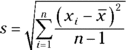
For detailed instructions on calculating the standard deviation, see Chapter 5.
The standard deviation is also used to describe where most of the data should fall, in a relative sense, compared to the average. For example, if your data have the form of a bell-shaped curve (also known as a normal distribution), about 95 percent of the data lie within two standard deviations of the mean. (This result is called the Empirical Rule, or the 68–95–99.7% rule. See Chapter 5 for more on this.)
The standard deviation is an important statistic, but it is often absent when statistical results are reported. Without it, you’re getting only part of the story about the data. Statisticians like to tell the story about a man named Dustin who had one foot in a bucket of ice water and the other foot in a bucket of boiling water. He said on average he felt just great! But think about the variability in the two temperatures for each of his feet. Closer to home, the average house price, for example, tells you nothing about the range of house prices you may encounter when house-hunting. The average salary may not fully represent what’s really going on in your company, if the salaries are extremely spread out.
Don’t be satisfied with finding out only the average; be sure to ask for the standard deviation as well. Without a standard deviation, you have no way of knowing how spread out the values may be. (If you’re talking starting salaries, for example, this could be very important!)
Percentile
You’ve probably heard references to percentiles before. If you’ve taken any kind of standardized test, you know that when your score was reported, it was presented to you with a measure of where you stood compared to the other people who took the test. This comparison measure was most likely reported to you in terms of a percentile. The percentile reported for a given score is the percentage of values in the data set that fall below that certain score. For example, if your score was reported to be at the 90th percentile, that means that 90 percent of the other people who took the test with you scored lower than you did (and 10 percent scored higher than you did). The median is right in the middle of a data set, so it represents the 50th percentile. For more specifics on percentiles, see Chapter 5.
Percentiles are used in a variety of ways for comparison purposes and to determine relative standing (that is, how an individual data value compares to the rest of the group). Babies’ weights are often reported in terms of percentiles, for example. Percentiles are also used by companies to see where they stand compared to other companies in terms of sales, profits, customer satisfaction, and so on.
Standard score
The standard score is a slick way to put results in perspective without having to provide a lot of details — something that the media loves. The standard score represents the number of standard deviations above or below the mean (without caring what that standard deviation or mean actually is).
For example, suppose Pat took the statewide 10th-grade test recently and scored 400. What does that mean? Not much, because you can’t put 400 into perspective. But knowing that Pat’s standard score on the test is +2 tells you everything. It tells you that Pat’s score is two standard deviations above the mean. (Bravo, Pat!) Now suppose Emily’s standard score is –2. In this case, this is not good (for Emily), because it means her score is two standard deviations below the mean.
The process of taking a number and converting it to a standard score is called standardizing. For the details on calculating and interpreting standard scores when you have a normal (bell-shaped) distribution, see Chapter 10.
Distribution and normal distribution
The distribution of a data set (or a population) is a listing or function showing all the possible values (or intervals) of the data and how often they occur. When a distribution of categorical data is organized, you see the number or percentage of individuals in each group. When a distribution of numerical data is organized, they’re often ordered from smallest to largest, broken into reasonably sized groups (if appropriate), and then put into graphs and charts to examine the shape, center, and amount of variability in the data.
The world of statistics includes dozens of different distributions for categorical and numerical data; the most common ones have their own names. One of the most well-known distributions is called the normal distribution, also known as the bell curve. The normal distribution is based on numerical data that is continuous; its possible values lie on the entire real number line. Its overall shape, when the data are organized in graph form, is a symmetric bell shape. In other words, most of the data are centered around the mean (giving you the middle part of the bell), and as you move farther out on either side of the mean, you find fewer and fewer values (representing the downward-sloping sides on either side of the bell).
The mean (and hence the median) is directly in the center of the normal distribution due to symmetry, and the standard deviation is measured by the distance from the mean to the inflection point (where the curvature of the bell changes from concave up to concave down). Figure 3-1 shows a graph of a normal distribution with mean 0 and standard deviation 1 (this distribution has a special name: the standard normal distribution or Z-distribution). The shape of the curve resembles the outline of a bell.
Because every distinct population of data has a different mean and standard deviation, an infinite number of different normal distributions exists, each with its own mean and its own standard deviation to characterize it. See Chapter 10 for plenty more on the normal and standard normal distributions.
Central Limit Theorem
The normal distribution is also used to help measure the accuracy of many statistics, including the mean, using an important tool in statistics called the Central Limit Theorem. This theorem gives you the ability to measure how much your sample mean will vary, without having to take any other sample means to compare it with (thankfully!). By taking this variability into account, you can now use your data to answer questions about the population, such as, “What’s the mean household income for the whole U.S.?” or “This report said 75 percent of all gift cards go unused; is that really true?” (These two particular analyses made possible by the Central Limit Theorem are called confidence intervals and hypothesis tests, respectively, and are described in Chapters 14 and 15, respectively.)
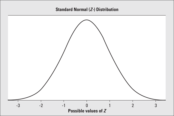
FIGURE 3-1: A standard normal (Z-) distribution has a bell-shaped curve with mean 0 and standard deviation 1.
The Central Limit Theorem (CLT for short) basically says that for non-normal data, your sample mean has an approximate normal distribution, no matter what the distribution of the original data looks like (as long as your sample size was large enough). And it doesn’t just apply to the sample mean; the CLT is also true for other sample statistics, such as the sample proportion (see Chapters 14 and 15). Because statisticians know so much about the normal distribution (see the preceding section), these analyses are much easier. See Chapter 12 for more on the Central Limit Theorem, known by statisticians as the “crown jewel in the field of all statistics.” (Should you even bother to tell them to get a life?)
z-values
If a data set has a normal distribution, and you standardize all the data to obtain standard scores, those standard scores are called z-values. All z-values have what is known as a standard normal distribution (or Z-distribution). The standard normal distribution is a special normal distribution with a mean equal to 0 and a standard deviation equal to 1.
The standard normal distribution is useful for examining the data and determining statistics like percentiles, or the percentage of the data falling between two values. So if researchers determine that the data have a normal distribution, they usually first standardize the data (by converting each data point into a z-value) and then use the standard normal distribution to explore and discuss the data in more detail. See Chapter 10 for more details on z-values.
Margin of error
You’ve probably heard or seen results like this: “This survey had a margin of error of plus or minus 3 percentage points.” What does this mean? Most surveys (except a census) are based on information collected from a sample of individuals, not the entire population. A certain amount of error is bound to occur — not in the sense of calculation error (although there may be some of that, too), but in the sense of sampling error, which is the error that occurs simply because the researchers aren’t asking everyone. The margin of error is supposed to measure the maximum amount by which the sample results are expected to differ from those of the actual population. Because the results of most survey questions can be reported in terms of percentages, the margin of error most often appears as a percentage, as well.
How do you interpret a margin of error? Suppose you know that 51 percent of people sampled say that they plan to vote for Senator Calculation in the upcoming election. Now, projecting these results to the whole voting population, you would have to add and subtract the margin of error and give a range of possible results in order to have sufficient confidence that you’re bridging the gap between your sample and the population. Assuming a margin of error of plus or minus 3 percentage points, you would be pretty confident that between 48 percent ![]() and 54 percent
and 54 percent ![]() of the population will vote for Senator Calculation in the election, based on the sample results. In this case, Senator Calculation may get slightly more or slightly less than the majority of votes and could either win or lose the election. This has become a familiar situation in recent years, when the media wants to report results on election night, but based on early exit polling results, the election is “too close to call.” For more about the margin of error, see Chapter 13.
of the population will vote for Senator Calculation in the election, based on the sample results. In this case, Senator Calculation may get slightly more or slightly less than the majority of votes and could either win or lose the election. This has become a familiar situation in recent years, when the media wants to report results on election night, but based on early exit polling results, the election is “too close to call.” For more about the margin of error, see Chapter 13.
The margin of error measures accuracy; it does not measure the amount of bias that may be present (you find a discussion of bias earlier in this chapter). Results that look numerically scientific and precise don’t mean anything if they are collected in a biased way.
Confidence interval
One of the biggest uses of statistics is to estimate a population parameter using a sample statistic. In other words, you use a number that summarizes a sample to help you guesstimate the corresponding number that summarizes the whole population (the definitions of parameter and statistic appear earlier in this chapter). You’re looking for a population parameter in each of the following questions:
- What’s the average household income in America? (Population = all households in America; parameter = average household income.)
- What percentage of all Americans watched the Academy Awards this year? (Population = all Americans; parameter = percentage who watched the Academy Awards this year.)
- What’s the average life expectancy of a baby born today? (Population = all babies born today; parameter = average life expectancy.)
- How effective is this new drug on adults with Alzheimer’s? (Population = all adults who have Alzheimer’s; parameter = percentage of these people who see improvement when taking this drug.)
It’s not possible to find these parameters exactly; they each require an estimate based on a sample. You start by taking a random sample from a population (say a sample of 1,000 households in America) and then finding the corresponding statistic from that sample (the sample’s mean household income). Because you know that sample results vary from sample to sample, you need to add a “plus or minus something” to your sample results if you want to draw conclusions about the whole population (all households in America). This “plus or minus” that you add to your sample statistic in order to estimate a parameter is the margin of error.
When you take a sample statistic (such as the sample mean or sample percentage) and you add/subtract a margin of error, you come up with what statisticians call a confidence interval. A confidence interval represents a range of likely values for the population parameter, based on your sample statistic. For example, suppose the average time it takes you to drive to work each day is 35 minutes, with a margin of error of plus or minus 5 minutes. You estimate that the average time driving to work would be anywhere from 30 to 40 minutes. This estimate is a confidence interval.
Some confidence intervals are wider than others (and wide isn’t good, because it means less accuracy). Several factors influence the width of a confidence interval, such as sample size, the amount of variability in the population being studied, and how confident you want to be in your results. (Most researchers are happy with a 95 percent level of confidence in their results.) For more on factors that influence confidence intervals, as well as instructions for calculating and interpreting confidence intervals, see Chapter 14.
Hypothesis testing
Hypothesis test is a term you probably haven’t run across in your everyday dealings with numbers and statistics. But I guarantee that hypothesis tests have been a big part of your life and your workplace, simply because of the major role they play in industry, medicine, agriculture, government, and a host of other areas. Any time you hear someone talking about their study showing a “statistically significant result,” you’re encountering a hypothesis test. (A statistically significant result is one that is unlikely to have occurred by chance, based on using a well-selected sample. See Chapter 15 for the full scoop.)
Basically, a hypothesis test is a statistical procedure in which data are collected from a sample and measured against a claim about a population parameter. For example, if a pizza delivery chain claims to deliver all pizzas within 30 minutes of placing the order, on average, you could test whether this claim is true by collecting a random sample of delivery times over a certain period and looking at the average delivery time for that sample. To make your decision, you must also take into account the amount by which your sample results can change from sample to sample (which is related to the margin of error).
Because your decision is based on a sample (even a well-selected one) and not the entire population, a hypothesis test can sometimes lead you to the wrong conclusion. However, statistics are all you have, and if done properly, they can give you a good chance of being correct. For more on the basics of hypothesis testing, see Chapter 15.
A variety of hypothesis tests are done in scientific research, including t-tests (comparing two population means), paired t-tests (looking at before/after data), and tests of claims made about proportions or means for one or more populations. For specifics on these hypothesis tests, see Chapter 16.
p-values
Hypothesis tests are used to test the validity of a claim that is made about a population. This claim that’s on trial, in essence, is called the null hypothesis. The alternative hypothesis is the one you would conclude if the null hypothesis is rejected. The evidence in the trial is your data and the statistics that go along with it. All hypothesis tests ultimately use a p-value to weigh the strength of the evidence (what the data are telling you about the population). The p-value is a number between 0 and 1 and is interpreted in the following way:
- A small p-value (such as less than 0.05) indicates strong evidence against the null hypothesis, so you reject it.
- A large p-value (greater than 0.05) indicates weak evidence against the null hypothesis, so you fail to reject it.
- p-values very close to the cutoff (0.05) are considered to be marginal (could go either way). Always report the p-value so your readers can draw their own conclusions.
For example, suppose a pizza place claims its delivery times are 30 minutes or less on average but you think it’s more than that. You conduct a hypothesis test because you believe the null hypothesis, H0, that the mean delivery time is 30 minutes max, is incorrect. Your alternative hypothesis (Ha) is that the mean time is greater than 30 minutes. You randomly sample some delivery times and run the data through the hypothesis test, and your p-value turns out to be 0.001, which is much less than 0.05. You conclude that the pizza place is wrong; their delivery times are in fact more than 30 minutes on average, and you want to know what they’re gonna do about it! (Of course, you could be wrong by having sampled an unusually high number of late pizzas just by chance; but whose side am I on?) For more on p-values, head to Chapter 15.
Statistical significance
Whenever data are collected to perform a hypothesis test, the researcher is typically looking for something out of the ordinary. (Unfortunately, research that simply confirms something that was already well known doesn’t make headlines.) Statisticians measure the amount by which a result is out of the ordinary using hypothesis tests (see Chapter 15). They use probability, the chance of how likely or unlikely some event is to occur, to put a number on how ordinary their result is. They define a statistically significant result as a result with a very small probability of happening just by chance, and provide a number called a p-value to reflect that probability (see the previous section on p-values).
For example, if a drug is found to be more effective at treating breast cancer than the current treatment, researchers say that the new drug shows a statistically significant improvement in the survival rate of patients with breast cancer. That means that based on their data, the difference in the overall results from patients using the new drug compared to those using the old treatment is so big that it would be hard to say it was just a coincidence. However, proceed with caution: You can’t say that these results necessarily apply to each individual or to each individual in the same way. For full details on statistical significance, see Chapter 15.
When you hear that a study’s results are statistically significant, don’t automatically assume that the study’s results are important. Statistically significant means the results were unusual, but unusual doesn’t always mean important. For example, would you be excited to learn that cats move their tails more often when lying in the sun than when lying in the shade, and that those results are statistically significant? This result may not even be important to the cat, much less anyone else!
Sometimes statisticians make the wrong conclusion about the null hypothesis because a sample doesn’t represent the population (just by chance). For example, a positive effect that was experienced by a sample of people who took the new treatment may have just been a fluke; or in the example in the preceding section, the pizza company really may have been delivering those pizzas on time and you just got an unlucky sample of slow ones. However, the beauty of research is that as soon as someone gives a press release saying that they found something significant, the rush is on to try to replicate the results, and if the results can’t be replicated, this probably means that the original results were wrong for some reason (including being wrong just by chance). Unfortunately, a press release announcing a “major breakthrough” tends to get a lot of play in the media, but follow-up studies refuting those results often don’t show up on the front page.
One statistically significant result shouldn’t lead to quick decisions on anyone’s part. In science, what most often counts is not a single remarkable study, but a body of evidence that is built up over time, along with a variety of well-designed follow-up studies. Take any major breakthroughs you hear about with a grain of salt and wait until the follow-up work has been done before using the information from a single study to make important decisions in your life. The results may not be replicable, and even if they are, you can’t know whether they necessarily apply to each individual.
Correlation, regression, and two-way tables
One of the most common goals of research is to find links between variables. For example,
- Which lifestyle behaviors increase or decrease the risk of cancer?
- What side effects are associated with this new drug?
- Can I lower my cholesterol by taking this new herbal supplement?
- Does spending a large amount of time on the Internet cause a person to gain weight?
Finding links between variables is what helps the medical world design better drugs and treatments, provides marketers with information on who is more likely to buy their products, and gives politicians information on which to build arguments for and against certain policies.
In the mega-business of looking for relationships between variables, you find an incredible number of statistical results — but can you tell what’s correct and what’s not? Many important decisions are made based on these studies, and it’s important to know what standards need to be met in order to deem the results credible, especially when a cause-and-effect relationship is being reported.
Chapter 19 breaks down all the details and nuances of plotting data from two numerical variables (such as dosage level and blood pressure), finding and interpreting correlation (the strength and direction of the linear relationship between x and y), finding the equation of a line that best fits the data (and when doing so is appropriate), and how to use these results to make predictions for one variable based on another (called regression). You also gain tools for investigating when a line fits the data well and when it doesn’t, and what conclusions you can make (and shouldn’t make) in the situations where a line does fit.
I cover methods used to look for and describe links between two categorical variables (such as the number of doses taken per day and the presence or absence of nausea) in detail in Chapter 20. I also provide info on collecting and organizing data into two-way tables (where the possible values of one variable make up the rows and the possible values for the other variable make up the columns), interpreting the results, analyzing the data from two-way tables to look for relationships, and checking for independence. And, as I do throughout this book, I give you strategies for critically examining results of these kinds of analyses for credibility.
Drawing Credible Conclusions
To perform statistical analyses, researchers use statistical software that depends on formulas. But formulas don’t know whether they are being used properly, and they don’t warn you when your results are incorrect. At the end of the day, computers can’t tell you what the results mean; you have to figure it out. Throughout this book you see what kinds of conclusions you can and can’t make after the analysis has been done. The following sections provide an introduction to drawing appropriate conclusions.
Reeling in overstated results
Some of the most common mistakes made in conclusions are overstating the results or generalizing the results to a larger group than was actually represented by the study. For example, Professor Lewis wants to know which Super Bowl commercials viewers liked best. He gathers 100 students from his class on Super Bowl Sunday and asks them to rate each commercial as it is shown. A top-five list is formed, and he concludes that all Super Bowl viewers liked those five commercials the best. But he really only knows which ones his students liked best — he didn’t study any other groups, so he can’t draw conclusions about all viewers.
Questioning claims of cause and effect
One situation in which conclusions cross the line is when researchers find that two variables are related (through an analysis such as regression; see the earlier section, “Correlation, regression, and two-way tables,” for more info) and then automatically leap to the conclusion that those two variables have a cause-and-effect relationship.
For example, suppose a researcher conducted a health survey and found that people who took vitamin C every day reported having fewer colds than people who didn’t take vitamin C every day. Upon finding these results, the researcher wrote a paper and gave a press release saying vitamin C prevents colds, using this data as evidence.
Now, while it may be true that vitamin C does prevent colds, this researcher’s study can’t claim that. This study was observational, which means they didn’t assign who would take vitamin C. For example, people who take vitamin C every day may be more health-conscious overall, washing their hands more often, exercising more, and eating better foods; all these behaviors may be helpful in reducing colds.
A controlled experiment can give you a cause-and-effect conclusion based on relationships you find. Observational studies can find cause-and-effect connections too, but it takes a larger body of evidence and more complex methods. (I discuss experiments in more detail earlier in this chapter.)
Becoming a Sleuth, Not a Skeptic
Statistics is about much more than numbers. To really “get” statistics, you need to understand how to make appropriate conclusions from studying data and be savvy enough to not believe everything you hear or read until you find out how the information came about, what was done with it, and how the conclusions were drawn. That’s something I discuss throughout the book.
Much of our advice is based on understanding the big picture as well as the details of tackling statistical problems and coming out a winner on the other side.
Becoming skeptical or cynical about statistics is very easy, especially after finding out what’s going on behind the scenes; don’t let that happen to you. You can find a lot of good information out there that can affect your life in a positive way. Find a good channel for your skepticism by setting two personal goals:
- To become a well-informed consumer of the statistical information you see every day.
- To establish job security by being the statistics “go-to” person who knows when and how to help others and when to find a statistician.
Through reading and using the information in this book, you’ll be confident in knowing you can make good decisions about statistical results. You’ll conduct your own statistical studies in a credible way. And you’ll be ready to tackle your next office project, critically evaluate that annoying political ad, or ace your next exam!