7 Opinionated optimization

This chapter covers

• Embracing premature optimization
• Taking a top-down approach to performance problems
• Optimizing CPU and I/O bottlenecks
• Making safe code faster and unsafe code safer

Programming literature on optimization always starts with a well-known quote by the famous computer scientist Donald Knuth: “Premature optimization is the root of all evil.” Not only is the statement wrong, but it’s also always misquoted. First, it’s wrong because everybody knows that the root of all evil is object-oriented programming since it leads to bad parenting and class struggles. Second, it’s wrong because the actual quote is more nuanced. This is almost another case of lorem ipsum, which is gibberish because it is quoted from the middle of an otherwise meaningful Latin text. Knuth’s actual statement is, “We should forget about small efficiencies, say about 97% of the time: premature optimization is the root of all evil. Yet we should not pass up our opportunities in that critical 3%.”¹

I claim that premature optimization is the root of all learning. Don’t hold yourself back from something you are so passionate about. Optimization is problem solving, and premature optimization creates nonexistent, hypothetical problems to solve, just like how chess players set up pieces to challenge themselves. It’s a good exercise. You can always throw away your work, as I’ve discussed in chapter 3, and keep the wisdom you gained. Exploratory programming is a legitimate way to improve your skills as long as you’re in control of the risks and the time. Don’t deprive yourself of learning opportunities.

That said, people try to discourage you from premature optimization for a reason. Optimization can bring rigidness to the code, making it harder to maintain. Optimization is an investment, and its return heavily depends on how long you can keep it. If specifications change, the optimizations you’ve performed may have you dug into a hole that is painful to get out of. More importantly, you could be trying to optimize for a problem that doesn’t exist in the first place, and making your code less reliable.

For example, you could have a file-copying routine, and you might know that the larger the buffer sizes you read and write at once, the faster the whole operation becomes. You might be tempted to just read everything in memory and write it to get the maximum possible buffer size. That might make your app consume unreasonable amounts of memory or cause it to crash when it tries to read an exceptionally large file. You need to understand the tradeoffs you’re making when you’re optimizing, which means you must correctly identify the problem you need to solve.

7.1 Solve the right problem

Slow performance can be fixed in many ways, and depending on the exact nature of the problem, the solution’s effectiveness and how much time you spend implementing it can vary drastically. The first step to understanding the true nature of a performance problem is to determine if there is a performance problem in the first place.

7.1.1 Simple benchmarking

Benchmarking is the act of comparing performance metrics. It may not help you identify the root cause of a performance problem, but it can help you identify its existence. Libraries like BenchmarkDotNet (https://github.com/dotnet/BenchmarkDotNet) make it extremely easy to implement benchmarks with safety measures to avoid statistical errors. But even if you don’t use any library, you can use a timer just to understand the execution time of the pieces of your code.

Something I have always wondered about is how much faster the Math.DivRem() function can be than a regular division-and-remainder operation. It’s been recommended that you use DivRem if you’re going to need the result of the division and the remainder at the same time, but I’ve never had the chance to test whether the claim holds up until now:

int division = a / b;
int remainder = a % b;

That code looks very primitive, and therefore it’s easy to assume that the compiler can optimize it just fine, while the Math.DivRem() version looks like an elaborate function call:

int division = Math.DivRem(a, b, out int remainder);

TIP You might be tempted to call the % operator the modulus operator, but it’s not. It’s the remainder operator in C or C#. There is no difference between the two for positive values, but negative values produce different results. For example, -7 % 3 is -1 in C#, while it’s 2 in Python.

You can create a benchmark suite right away with BenchmarkDotNet, and it’s great for microbenchmarking, a type of benchmarking in which you measure small and fast functions because either you’re out of options or your boss is on vacation. BenchmarkDotNet can eliminate the measurement errors related to fluctuations or the function call overhead. In listing 7.1, you can see the code that uses BenchmarkDotNet to test the speed of DivRem versus manual division/remainder operations. We basically create a new class that describes the benchmark suite with benchmarked operations marked with [Benchmark] attributes. BenchmarkDotNet itself figures out how many times it needs to call those functions to get accurate results because a one-time measurement or running only a few iterations of benchmarks is susceptible to errors. We use multitasking operating systems, and other tasks running in the background can impact the performance of the code we’re benchmarking on these systems. We mark the variables used in calculation with the [Params] attribute to prevent the compiler from eliminating the operations it deems unnecessary. Compilers are easily distracted, but they’re smart.

Listing 7.1 Example BenchmarkDotNet code

public class SampleBenchmarkSuite {
  [Params(1000)]                       ❶
  public int A;
 
  [Params(35)]                         ❶
  public int B;
 
  [Benchmark]                          ❷
  public int Manual() {
    int division = A / B;
    int remainder = A % B;
    return division + remainder;       ❸
  }
 
  [Benchmark]                          ❷
  public int DivRem() {
    int division = Math.DivRem(A, B, out int remainder);
    return division + remainder;       ❸
  }
}

❶ We’re avoiding compiler optimizations.

❷ Attributes mark the operations to be benchmarked.

❸ We return values, so the compiler doesn’t throw away computation steps.

You can run these benchmarks simply by creating a console application and adding a using line and Run call in your Main method:

using System;
using System.Diagnostics;
using BenchmarkDotNet.Running;
 
namespace SimpleBenchmarkRunner {
  public class Program {
    public static void Main(string[] args) {
      BenchmarkRunner.Run<SampleBenchmarkSuite>();
    }
  }
}

If you run your application, the Benchmark results will be shown after a minute of running:

| Method |    a |  b |     Mean |     Error |    StdDev |
|------- |----- |--- |---------:|----------:|----------:|
| Manual | 1000 | 35 | 2.575 ns | 0.0353 ns | 0.0330 ns |
| DivRem | 1000 | 35 | 1.163 ns | 0.0105 ns | 0.0093 ns |

It turns out Math.DivRem() is twice as fast as performing division and remainder operations separately. Don’t be alarmed by the Error column because it’s only a statistical property to help the reader assess accuracy when BenchmarkDotNet doesn’t have enough confidence in the results. It’s not the standard error, but rather, half of the 99.9% confidence interval.

Although BenchmarkDotNet is dead simple and comes with features to reduce statistical errors, you may not want to deal with an external library for simple benchmarking. In that case, you can just go ahead and write your own benchmark runner using a Stopwatch, as in listing 7.2. You can simply iterate in a loop long enough to get a vague idea about the relative differences in the performance of different functions. We’re reusing the same suite class we created for BenchmarkDotNet, but we’re using our own loops and measurements for the results.

Listing 7.2 Homemade benchmarking

private const int iterations = 1_000_000_000;
 
private static void runBenchmarks() {
  var suite = new SampleBenchmarkSuite {
    A = 1000,
    B = 35
  };
 
  long manualTime = runBenchmark(() => suite.Manual());
  long divRemTime = runBenchmark(() => suite.DivRem());
 
  reportResult("Manual", manualTime);
  reportResult("DivRem", divRemTime);
}
 
private static long runBenchmark(Func<int> action) {
  var watch = Stopwatch.StartNew();
  for (int n = 0; n < iterations; n++) {
    action();                             ❶
  }
  watch.Stop();
  return watch.ElapsedMilliseconds;
}
 
private static void reportResult(string name, long milliseconds) {
  double nanoseconds = milliseconds * 1_000_000;
  Console.WriteLine("{0} = {1}ns / operation",
    name,
    nanoseconds / iterations);
}

❶ We call the benchmarked code here.

When we run it, the result is relatively the same:

Manual = 4.611ns / operation
DivRem = 2.896ns / operation

Note that our benchmarks don’t try to eliminate function call overhead or the overhead of the for loop itself, so they seem to be taking longer, but we successfully observe that DivRem is still twice as fast as manual division-and-remainder operations.

7.1.2 Performance vs. responsiveness

Benchmarks can only report relative numbers. They can’t tell you if your code is fast or slow, but they can tell you if it’s slower or faster than some other code. A general principle about slowness from a user’s point of view is that any action that takes more than 100 ms feels delayed, and any action that takes more than 300 ms is considered sluggish. Don’t even think about taking a full second. Most users will leave a web page or an app if they have to wait for more than three seconds. If a user’s action takes more than five seconds to respond, it might as well take the lifetime of the universe—it doesn’t matter at that point. Figure 7.1 illustrates this.

Figure 7.1 Response delays vs. frustration

Obviously, performance isn’t always about responsiveness. In fact, being a responsive app might require performing an operation more slowly. For example, you might have an app that replaces faces in a video with your face using machine learning. Because such a task is computationally intensive, the fastest way to calculate it is to do nothing else until the job’s done. But that would mean a frozen UI, which would make the user think something’s wrong and persuade them to quit the app. So instead of doing the computation as fast as you can, you instead spare some of the computational cycles to show a progress bar, perhaps to calculate estimated time remaining and to show a nice animation that can entertain users while they’re waiting. In the end, you have slower code, but a more successful outcome.

That means that even if benchmarks are relative, you can still have some understanding of slowness. Peter Norvig came up with the idea in his blog² of listing latency numbers to have a context of how things can be slower by orders of magnitude in different contexts. I create a similar table with my own back-of-the-envelope calculations in table 7.1. You can come up with your own numbers by looking at this.

Table 7.1 Latency numbers in various contexts

Latency affects performance too, not just user experience. Your database resides on a disk, and your database server resides on a network. That means that even if you write the fastest SQL queries and define the fastest indexes on your database, you’re still bound by the laws of physics, and you can’t get any result faster than a millisecond. Every millisecond you spend eats into your total budget, which is ideally less than 300 ms.

7.2 Anatomy of sluggishness

To understand how to improve performance, you must first understand how performance fails. As we’ve seen, not all performance problems are about speed—some are about responsiveness. The speed part, though, is related to how computers work in general, so it’s a good idea to acquaint yourself with some low-level concepts. This will help you understand the optimization techniques I’ll discuss later in the chapter.

CPUs are chips that process instructions they read from RAM and perform them repetitively in a never-ending loop. You can imagine it like a wheel turning, and every rotation of the wheel typically performs another instruction, as depicted in figure 7.2. Some operations can take multiple turns, but the basic unit is a single turn, popularly known as a clock cycle, or a cycle for short.

Figure 7.2 The 20,000-feet anatomy of a single CPU cycle

The speed of a CPU, typically expressed in hertz, indicates how many clock cycles it can process in a second. The first electronic computer, ENIAC, could process 100,000 cycles a second, shortened to 100 KHz. The antique 4 MHz Z80 CPU in my 8-bit home computer back in the 1980s could only process 4 million cycles per second. A modern 3.4 GHz AMD Ryzen 5950X CPU can process 3.4 billion cycles in a second on each of its cores. That doesn’t mean CPUs can process that many instructions, because first, some instructions take more than one clock cycle to complete, and second, modern CPUs can process multiple instructions in parallel on a single core. Thus, sometimes CPUs can even run more instructions than what their clock speed allows.

Some CPU instructions can also take an arbitrary amount of time depending on their arguments, such as block memory copy instructions. Those take O(N) time based on how large the block is.

Basically, every performance problem related to code speed comes down to how many instructions are executed and for how many times. When you optimize code, what you’re trying to do is either reduce the number of instructions executed or use a faster version of an instruction. The DivRem function runs faster than division and remainder because it gets converted into instructions that take fewer cycles.

7.3 Start from the top

The second-best way to reduce the number of instructions executed is to choose a faster algorithm. The best way obviously is to delete the code entirely. I’m serious: delete the code you don’t need. Don’t keep unneeded code in the codebase. Even if it doesn’t degrade the performance of the code, it degrades the performance of developers, which eventually degrades the performance of the code. Don’t even keep commented-out code. Use the history features of your favorite source control system like Git or Mercurial to restore old code. If you need the feature occasionally, put it behind configuration instead of commenting it out. This way, you won’t be surprised when you finally blow the dust off the code and it won’t compile at all because everything’s changed. It’ll remain current and working.

As I pointed out in chapter 2, a faster algorithm can make a tremendous difference, even if it’s implemented in a poorly optimized way. So first ask yourself, “Is this the best way to do this?” There are ways to make badly implemented code faster, but nothing beats solving the problem at the top, as in the broadest scope, the scenario itself, and delve deeper until you figure out the actual location of the problem. This way is usually faster, and the result ends up being way more easily maintained.

Consider an example in which users complain that viewing their profile on the app is slow, and you can reproduce the problem yourself. The performance problem can come from either the client or the server. So you start from the top: you first identify which major layer the problem appears in by eliminating one of the two layers the problem can possibly be in. If a direct API call doesn’t have the same problem, the problem must be in the client, or, otherwise, in the server. You continue on this path until you identify the actual problem. In a sense, you’re doing a binary search, as shown in figure 7.3.

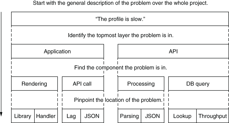
Figure 7.3 A top-down approach for identifying the root cause

When you follow a top-down approach, you’re guaranteed to find the root cause of the problem in an efficient way, instead of guessing. Since you do a binary search manually here, you’re now using algorithms in real life to make your life easier, so, good job! When you determine where the problem happens, check any red flags for obvious code complexity. You can identify patterns that might be causing more complex code to execute when a simple one could suffice. Let’s go over some of them.

7.3.1 Nested loops

One of the easiest ways to slow down code is to put it inside another loop. When writing code in nested loops, we underestimate the effects of multiplication. Nested loops aren’t always visible, either. To expand on our example about the slow user profile, suppose you found the problem in the backend code that generates the profile data. There is a function that returns the badges a user has and shows them on their profile. Some sample code might look like this:

public IEnumerable<string> GetBadgeNames() {
  var badges = db.GetBadges();
  foreach (var badge in badges) {
    if (badge.IsVisible) {
      yield return badge.Name;
    }
  }
}

There are no apparent nested loops here. As a matter of fact, it’s possible to write the same function with LINQ without any loops at all, but with the same slowness problem:

public IEnumerable<string> GetBadgesNames() {
  var badges = db.GetBadges();
  return badges
    .Where(b => b.IsVisible)
    .Select(b => b.Name);
}

Where is the inner loop? That’s something you’ll have to ask yourself over the course of your programming career. The culprit is the IsVisible property because we just don’t know what it’s doing underneath.

Properties in C# were invented because the developers of the language were tired of writing get in front of every function name regardless of how simple it might be. As a matter of fact, property code is converted to functions when compiled, with get_ and set_ prefixes added to their name. The upside of using properties is that they allow you to change how a field-looking member in a class functions without breaking compatibility. The downside of properties is that they conceal potential complexity. They look like simple fields, basic memory access operations, which might make you assume that calling a property may not be expensive at all. Ideally, you should never put computationally intensive code inside properties, but it’s impossible for you to know whether someone else has done it, at least not without looking.

When we look at the source of the IsVisible property of the Badge class, we can see it’s more expensive than it looks:

public bool IsVisible {
  get {
    var visibleBadgeNames = db.GetVisibleBadgeNames();
    foreach (var name in visibleBadgeNames) {
      if (this.Name == name) {
        return true;
      }
    }
    return false;
  }
}

This property, without any shame, dares to call the database to retrieve the list of visible badge names and compares them in a loop to see if our supposed badge is one of the visible ones. There are too many sins in that code to explain, but your first lesson is to beware of properties. They contain logic, and their logic may not always be simple.

There are many optimization opportunities in the IsVisible property, but the first and foremost one is to not retrieve the list of visible badge names every time the property is called. You could keep them in a static list that’s retrieved only once, assuming the list rarely changes and you can afford a restart when it happens. You can also do caching, but I’ll get to that later. That way, you could reduce the property code to this:

private static List<string> visibleBadgeNames = getVisibleBadgeNames();
 
public bool IsVisible {
  get {
    foreach (var name in visibleBadgeNames) {
      if (this.Name == name) {
        return true;
      }
    }
    return false;
  }
}

The good thing about keeping a list is that it already has a Contains method so you can eliminate the loop in IsVisible:

public bool IsVisible {
  get => visibleBadgeNames.Contains(this.Name);
}

The inner loop has finally disappeared, but we still haven’t destroyed its spirit. We need to salt and burn its bones. Lists in C# are essentially arrays, and they have O(N) lookup complexity. That means our loop hasn’t gone away, but has only moved inside another function, in this case, List<T>.Contains(). We can’t reduce complexity by eliminating the loop—we have to change our lookup algorithm too.

We can sort the list and do a binary search to reduce lookup performance to O(logN), but luckily, we’ve read chapter 2, and we know how the HashSet<T> data structure can provide a much better O(1) lookup performance, thanks to looking up an item’s location using its hash. Our property code has finally started to look sane:

private static HashSet<string> visibleBadgeNames = getVisibleBadgeNames();
 
public bool IsVisible {
  get => visibleBadgeNames.Contains(this.Name);
}

We haven’t done any benchmarking on this code, but looking at computational complexity pain points can provide you good insight, as you can see in this example. You should still always test whether your fix performs better because code will always contain surprises and dark corners that might ambush you.

The story of the GetBadgeNames() method doesn’t end here. There are other questions to ask, like why the developer keeps a separate list of visible badge names instead of a single bit flag in the Badge record on the database or why they don’t simply keep them in a separate table and join them while querying the database. But as far as nested loops are concerned, it has probably become orders of magnitude faster now.

7.3.2 String-oriented programming

Strings are extremely practical. They are readable, they can hold any kind of text, and they can be manipulated easily. I have already discussed how using the right type can give better performance than using a string, but there are subtle ways that strings can seep into your code.

One of the common ways that strings can be used unnecessarily is to assume every collection is a string collection. For example, if you want to keep a flag in an HttpContext .Items or ViewData container, it’s common to find someone writing something like

HttpContext.Items["Bozo"] = "true";

You find them later checking the same flag like this:

if ((string)HttpContext.Items["Bozo"] == "true") {
. . .
}

The typecast to string is usually added after the compiler warns you, “Hey, are you sure you want to do this? This isn’t a string collection.” But the whole picture that the collection is actually an object collection is usually missed. You could, in fact, fix the code by simply using a Boolean variable instead:

HttpContext.Items["Bozo"] = true;

Check the value with

if ((bool?)HttpContext.Items["Bozo"] == true) {
...
}

This way, you avoid storage overhead, parsing overhead, and even occasional typos like typing True instead of true.

The actual overhead of these simple mistakes is minuscule, but when they become habits, it can accumulate significantly. It’s impossible to fix the nails on a leaking ship, but nailing them the right way when you build it can help you stay afloat.

7.3.3 Evaluating 2b || !2b

Boolean expressions in if statements are evaluated in the order they’re written. The C# compiler generates smart code for evaluation to avoid unnecessarily evaluating cases altogether. For example, remember our awfully expensive IsVisible property? Consider this check:

if (badge.IsVisible && credits > 150_000) {

An expensive property gets evaluated before a simple value check. If you’re calling this function mostly with values of x less than 150,000, IsVisible wouldn’t be called most of the time. You can simply swap the places of expressions:

if (credits > 150_000 && badge.IsVisible) {

This way, you wouldn’t be running an expensive operation unnecessarily. You can also apply this with logical OR operations (||). In that case, the first expression that returns true would prevent the rest of the expression from being evaluated. Obviously, in real life, having that kind of expensive property is rare, but I recommend sorting expressions based on operand types:

1. Variables

2. Fields

3. Properties

4. Method calls

Not every Boolean expression can be safely moved around the operators. Consider this:

if (badge.IsVisible && credits > 150_000 || isAdmin) {

You can’t simply move isAdmin to the beginning because it would change the evaluation. Make sure you don’t accidentally break the logic in the if statement while you’re optimizing Boolean evaluation.

7.4 Breaking the bottle at the neck

There are three types of delays in software: CPU, I/O, and human. You can optimize each category by finding a faster alternative, parallelizing the tasks, or removing them from the equation.

When you’re sure you’re using an algorithm or a method that’s suitable for the job, it finally comes down to how you can optimize the code itself. To evaluate your options for optimizations, you need to be aware of the luxuries that CPUs provide you.

7.4.1 Don’t pack data

Reading from a memory address, say, 1023, can take more time than reading from memory address 1024 because CPUs can incur a penalty when reading from unaligned memory addresses. Alignment in that sense means a memory location on the multiples of 4, 8, 16, and so forth, at least the word size of the CPU, as seen in figure 7.4. On some older processors, the penalty for accessing unaligned memory is death by a thousand small electrical shocks. Seriously, some CPUs don’t let you access unaligned memory at all, such as the Motorola 68000 that is used in Amiga and some ARM-based processors.

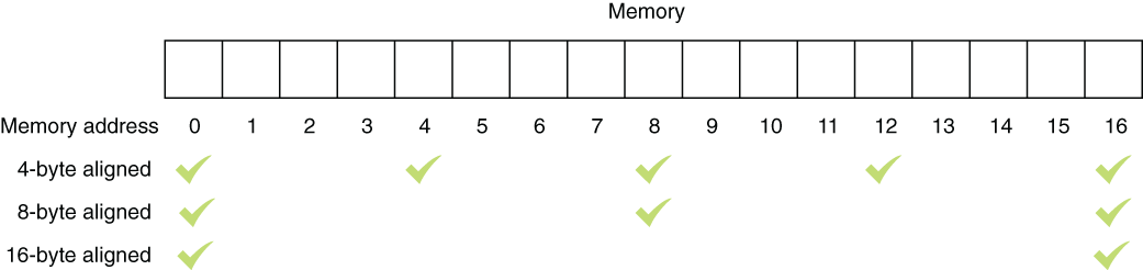
Figure 7.4 Memory address alignment

Thankfully, we have compilers, and they usually take care of the alignment stuff. But it’s possible to override the behavior of the compiler, and it still may not feel that something’s wrong: you’re storing more stuff in a small space, there is less memory to read, so it should be faster. Consider the data structure in listing 7.4. Because it’s a struct, C# will apply alignment only based on some heuristics, and that can mean no alignment at all. You might be tempted to keep the values in bytes so it becomes a small packet to pass around.

Listing 7.3 A packed data structure

struct UserPreferences {
  public byte ItemsPerPage;
  public byte NumberOfItemsOnTheHomepage;
  public byte NumberOfAdClicksICanStomach;
  public byte MaxNumberOfTrollsInADay;
  public byte NumberOfCookiesIAmWillingToAccept;
  public byte NumberOfSpamEmailILoveToGetPerDay;
}

But, since memory accesses to unaligned boundaries are slower, your storage savings are offset by the access penalty to each member in the struct. If you change the data types in the struct from byte to int and create a benchmark to test the difference, you can see that byte access is almost twice as slow, even though it occupies a quarter of the memory, as shown in table 7.2.

Table 7.2 Difference between aligned and unaligned member access

The moral of the story is to avoid optimizing memory storage unnecessarily. There are benefits to doing it in certain cases: for example, when you want to create an array of a billion numbers, the difference between byte and int can become three gigabytes. Smaller sizes can also be preferable for I/O, but, otherwise, trust the memory alignment. The immutable law of benchmarking is, “Measure twice, cut once, then measure again, and you know what, let’s go easy on the cutting for a while.”

7.4.2 Shop local

Caching is about keeping frequently used data at a location that can be accessed faster than where it usually resides. CPUs have their own cache memories with different speeds, but all are faster than RAM itself. I won’t go into the technical details of how cache is structured, but basically, CPUs can read memory in their cache much faster than regular memory in RAM. That means, for example, that sequential reads are faster than random reads around the memory. For example, reading an array sequentially can be faster than reading a linked list sequentially, although both take O(N) time to read end to end, and arrays can perform better than linked lists. The reason is that there is a higher chance of the next element being in the cached area of the memory. The elements of linked lists, on the other hand, are scattered around in the memory because they are separately allocated.

Suppose you have a CPU with a 16-byte cache, and you have both an array of three integers and a linked list of three integers. In figure 7.5, you can see that reading the first element of the array would also trigger loading the rest of the elements into the CPU cache, while traversing the linked list would cause a cache miss and force the new region to be loaded into the cache.

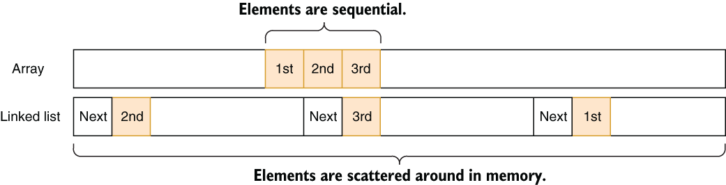
Figure 7.5 Array vs. linked list cache locality

CPUs usually bet that you’re reading data sequentially. That doesn’t mean linked lists don’t have their uses. They have excellent insert/delete performance and less memory overhead when they are growing. Array-based lists need to reallocate and copy buffers when they’re growing, which is terribly slow, so they allocate more than they need, which can cause disproportionate memory use in large lists. In most cases, though, a list would serve you fine, and it might well be faster for reading.

7.4.3 Keep dependent works separated

A single CPU instruction is processed by discrete units on the processor. For example, one unit is responsible for decoding the instruction, while another is responsible for memory access. But since a decoder unit needs to wait for an instruction to complete, it can do other decoding work for the next instruction while memory access is running. That technique is called pipelining, and it means the CPU can execute multiple instructions in parallel on a single core as long as the next instruction doesn’t depend on the result of the previous one.

Consider an example: you need to calculate a checksum in which you simply add the values of a byte array to get a result, as in listing 7.4. Normally, checksums are used for error detection, and adding numbers can be the worst implementation, but we’ll assume that it was a government contract. When you look at the code, it constantly updates the value of the result. Therefore, every calculation depends on i and result. That means the CPU cannot parallelize any work, because it depends on an operation.

Listing 7.4 A simple checksum

public int CalculateChecksum(byte[] array) {
  int result = 0;
  for (int i = 0; i < array.Length; i++) {
    result = result + array[i];             ❶
  }
  return result;
}

❶ Depends on both i and the previous value of the result

There are ways to reduce dependencies or at least reduce the blocking impact of the instruction flow. One is to reorder instructions to increase the gap between dependent code so an instruction doesn’t block the following one in the pipeline due to the dependency on the result of the first operation.

Since addition can be done in any order, we can split the addition into four parts in the same code and let the CPU parallelize the work. We can implement the task as I have in the following listing. This code contains more instructions, but four different result accumulators can now complete the checksum separately and later be summed. We then sum the remaining bytes in a separate loop.

Listing 7.5 Parallelizing work on a single core

public static int CalculateChecksumParallel(byte[] array) {
  int r0 = 0, r1 = 0, r2 = 0, r3 = 0;                       ❶
  int len = array.Length;
  int i = 0;
  for (; i < len - 4; i += 4) {
    r0 += array[i + 0];                                     ❷
    r1 += array[i + 1];                                     ❷
    r2 += array[i + 2];                                     ❷
    r3 += array[i + 3];                                     ❷
  }
  int remainingSum = 0;
  for (; i < len; i++) {                                    ❸
    remainingSum += i;
  }
  return r0 + r1 + r2 + r3 + remainingSum;                  ❹
}

❶ The four accumulators!

❷ These calculations are independent of each other.

❸ Calculate the sum of the remaining bytes.

❹ Bring everything together.

We’re doing a lot more work than in the simpler code in listing 7.4, and yet, this process turns out be 15% faster on my machine. Don’t expect magic from such a micro-optimization, but you’ll love it when it helps you tackle CPU-intensive code. The main takeaway is that reordering code—and even removing dependencies in code—can improve your code’s speed because dependent code can clog up the pipeline.

7.4.4 Be predictable

The most upvoted, the most popular question in the history of Stack Overflow is, “Why is processing a sorted array faster than processing an unsorted array?”³ To optimize execution time, CPUs try to act preemptively ahead of the running code to make preparations before there is a need. One technique CPUs employ is called branch prediction. Such code is just a sugarcoated version of comparisons and branches:

if (x == 5) {
  Console.WriteLine("X is five!");
} else {
  Console.WriteLine("X is something else");
}

The if statement and curly braces are the elements of structured programming. They are a sugarcoated version of what the CPU processes. Behind the scenes, the code gets converted into a low-level code like this during the compilation phase:

  compare x with 5
  branch to ELSE if not equal
  write "X is five"
  branch to SKIP_ELSE
ELSE:
  write "X is something else"
SKIP_ELSE:

I’m just paraphrasing here because the actual machine code is more cryptic, but this isn’t entirely inaccurate. Regardless of how elegant the design you create with your code is, it eventually becomes a bunch of comparison, addition, and branch operations. Listing 7.6 shows the actual assembly output for x86 architecture for the same code. It might feel more familiar after you’ve seen the pseudocode. There is an excellent online tool at sharplab.io that lets you see the assembly output of your C# program. I hope it will outlive this book.

Listing 7.6 Actual assembly code for our comparison

        cmp ecx, 5                     ❶
        jne ELSE                       ❷
        mov ecx, [0xf59d8cc]           ❸
        call System.Console.WriteLine(System.String)
        ret                            ❹
ELSE:   mov ecx, [0xf59d8d0]           ❺
        call System.Console.WriteLine(System.String)
        ret                            ❹

❶ Compare instruction

❷ Branching instruction (Jump if Not Equal)

❸ Pointer for the string “X is 5”

❹ Return instruction

❺ Pointer for the string “X is something else”

    let a, 42
some_label:
    decrement a
    compare a, 0
    jump_if_not_equal some_label

    mov al, 42
some_label:
    dec al
    cmp al, 0
    jne some_label

    mov r0, #42
some_label:
    sub r0, r0, #1
    cmp r0, #0
    bne some_label

A CPU can’t know if a comparison will be successful before it’s executed, but thanks to branch prediction, it can make a strong guess based on what it observes. Based on its guesses, the CPU makes a bet and starts processing instructions from that branch it predicted, and if it’s successful in its prediction, everything is already in place, boosting the performance.

That’s why processing an array with random values can be slower if it involves comparisons of values: branch prediction fails spectacularly in that case. A sorted array performs better because the CPU can predict the ordering properly and predict the branches correctly.

Keep that in mind when you’re processing data. The fewer surprises you give the CPU, the better it will perform.

7.4.5 SIMD

CPUs also support specialized instructions that can perform computations on multiple data at the same time with a single instruction. That technique is called single instruction, multiple data (SIMD). If you want to perform the same calculation on multiple variables, SIMD can boost its performance significantly on supported architectures.

SIMD works pretty much like multiple pens taped together. You can draw whatever you want, but the pens will all perform the same operation on different coordinates of the paper. An SIMD instruction will perform an arithmetic computation on multiple values, but the operation will remain constant.

C# provides SIMD functionality via Vector types in the System.Numerics namespace. Since every CPU’s SIMD support is different, and some CPUs don’t support SIMD at all, you first must check whether it’s available on the CPU:

if (!Vector.IsHardwareAccelerated) {
  . . . non-vector implementation here . . .
}

Then you need to figure out how many of a given type the CPU can process at the same time. That changes from processor to processor, so you have to query it first:

int chunkSize = Vector<int>.Count;

In this case, we’re looking to process int values. The number of items the CPU can process can change based on the data type. When you know the number of elements you can process at a time, you can go ahead and process the buffer in chunks.

Consider that we’d like to multiply values in an array. Multiplication of a series of values is a common problem in data processing, whether it’s changing the volume of a sound recording or adjusting the brightness of an image. For example, if you multiply pixel values in an image by 2, it becomes twice as bright. Similarly, if you multiply voice data by 2, it becomes twice as loud. A naive implementation would look like that in the following listing. We simply iterate over the items and replace the value in place with the result of the multiplication.

Listing 7.7 Classic in-place multiplication

public static void MultiplyEachClassic(int[] buffer, int value) {
  for (int n = 0; n < buffer.Length; n++) {
    buffer[n] *= value;
  }
}

When we use the Vector type to make these calculations instead, our code becomes more complicated, and it looks slower, to be honest. You can see the code in listing 7.8. We basically check for SIMD support and query the chunk size for integer values. We later go over the buffer at the given chunk size and copy the values into vector registers by creating instances of Vector<T>. That type supports standard arithmetic operators, so we simply multiply the vector type with the number given. It will automatically multiply all of the elements in the chunk in a single go. Notice that we declare the variable n outside the for loop because we’re starting from its last value in the second loop.

Listing 7.8 “We’re not in Kansas anymore” multiplication

public static void MultiplyEachSIMD(int[] buffer, int value) {
  if (!Vector.IsHardwareAccelerated) {
    MultiplyEachClassic(buffer, value);          ❶
  }
 
  int chunkSize = Vector<int>.Count;             ❷
  int n = 0;
  for (; n < buffer.Length - chunkSize; n += chunkSize) {
    var vector = new Vector<int>(buffer, n);     ❸
    vector *= value;                             ❹
    vector.CopyTo(buffer, n);                    ❺
  }
 
  for (; n < buffer.Length; n++) {               ❻
    buffer[n] *= value;                          ❻
  }                                              ❻
}

❶ Call the classic implementation if SIMDs are not supported.

❷ Query how many values SIMD can process at once.

❸ Copy the array segment into SIMD registers.

❹ Multiply all values at once.

❺ Replace the results.

❻ Process the remaining bytes the classic way.

It looks like too much work, doesn’t it? Yet, the benchmarks are impressive, as shown in table 7.3. In this case, our SIMD-based code is twice as fast as the regular code. Based on the data types you process and operations you perform on the data, it can be much higher.

Table 7.3 The SIMD difference

You can consider SIMD when you have a computationally intensive task and you need to perform the same operation on multiple elements at the same time.

7.5 1s and 0s of I/O

I/O encompasses everything a CPU communicates with the peripheral hardware, be it disk, network adapter, or even GPU. I/O is usually the slowest link on the performance chain. Think about it: a hard drive is actually a rotating disk with a spindle seeking over the data. It’s basically a robotic arm constantly moving around. A network packet can travel at the speed of light, and yet, it would still take it more than 100 milliseconds to rotate the earth. Printers are especially designed to be slow, inefficient, and anger inducing.

You can’t make I/O itself faster most of the time because its slowness arises from physics, but the hardware can run independently of the CPU, so it can work while the CPU is doing other stuff. That means you can overlap the CPU and I/O work and complete an overall operation in a smaller timeframe.

7.5.1 Make I/O faster

Yes, I/O is slow due to the inherent limitations of hardware, but it can be made faster. For example, every read from a disk incurs an operating system call overhead. Consider file-copy code like that in the following listing. It’s pretty much straightforward. It copies every byte read from the source file and writes those bytes to the destination file.

Listing 7.9 Simple file copy

public static void Copy(string sourceFileName,
  string destinationFileName) {
 
  using var inputStream = File.OpenRead(sourceFileName);
  using var outputStream = File.Create(destinationFileName);
  while (true) {
    int b = inputStream.ReadByte();      ❶
    if (b < 0) {
      break;
    }
    outputStream.WriteByte((byte)b);     ❷
  }
}

❶ Read the byte.

❷ Write the byte.

The problem is that every system call implies an elaborate ceremony. The ReadByte() function here calls the operating system’s read function. The operating system calls the switch-to-kernel mode. That means the CPU changes its execution mode. The operating system routine looks up the file handle and necessary data structures. It checks whether the I/O result is already in cache. If it’s not, it calls the relevant device drivers to perform the actual I/O operation on the disk. The read portion of the memory gets copied to a buffer in the process’s address space. These operations happen lightning fast, and it can become significant when you just read one byte.

Many I/O devices read/write in blocks called block devices. Network and storage devices are usually block devices. The keyboard is a character device because it sends one character at a time. Block devices can’t read less than the size of a block, so it doesn’t make sense to read anything less than a typical block size. For example, a hard drive can have a sector size of 512 bytes, making it a typical block size for disks. Modern disks can have larger block sizes, but let’s see how much performance can be improved simply by reading 512 bytes. The following listing shows the same copy operation that takes a buffer size as a parameter and reads and writes using that chunk size.

Listing 7.10 File copy using larger buffers

public static void CopyBuffered(string sourceFileName,
  string destinationFileName, int bufferSize) {
 
  using var inputStream = File.OpenRead(sourceFileName);
  using var outputStream = File.Create(destinationFileName);
  var buffer = new byte[bufferSize];
  while (true) {
    int readBytes = inputStream.Read(buffer, 0, bufferSize);     ❶
    if (readBytes == 0) {
      break;
    }
    outputStream.Write(buffer, 0, readBytes);                    ❷
  }
}

❶ Read bufferSize bytes at once.

❷ Write bufferSize bytes at once.

If we write a quick benchmark that tests against the byte-based copy function and the buffered variant with different buffer sizes, we can see the difference that reading large chunks at a time makes. You can see the results in table 7.4.

Table 7.4 Effect of buffer size on I/O performance

Even using a 512-byte buffer makes a tremendous difference—the copy operation becomes six times faster. Yet, increasing it to 256 KB makes the most difference, and making it anything larger yields only marginal improvement. I ran these benchmarks on a Windows machine, and Windows I/O uses 256 KB as the default buffer size for its I/O operations and cache management. That’s why the returns suddenly become marginal after 256 KB. In the same way as food package labels say “actual contents may vary,” your actual experience on your operating system may vary. Consider finding the ideal buffer size when you’re working with I/O, and avoid allocating more memory than you need.

7.5.2 Make I/O non-blocking

One of the most misunderstood concepts in programming is asynchronous I/O. It’s often confused with multithreading, which is a parallelization model to make any kind of operation faster by letting a task run on separate cores. Asynchronous I/O (or async I/O for short) is a parallelization model for I/O-heavy operations only, and it can work on a single core. Multithreading and async I/O can also be used together because they address different use cases.

I/O is naturally asynchronous because the external hardware is almost always slower than the CPU, and the CPU doesn’t like waiting and doing nothing. Mechanisms like interrupts and direct memory access (DMA) were invented to allow hardware to signal the CPU when an I/O operation is complete, so the CPU can transfer the results. That means that when an I/O operation is issued to the hardware, the CPU can continue executing other stuff while the hardware is doing its work, and the CPU can check back when the I/O operation is complete. This mechanism is the foundation of async I/O.

Figure 7.6 gives an idea of how both types of parallelization work. In both illustrations, the second computational code (CPU Op #2) is dependent on the result of the first I/O code (I/O Op #1). Because computational code can’t be parallelized on the same thread, they execute in tandem and therefore take longer than multi-threading on a four-core machine. On the other hand, you still gain significant parallelization benefits without consuming threads or occupying cores.

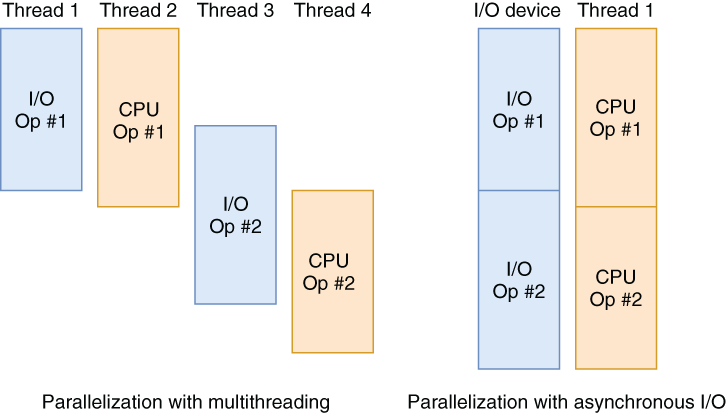
Figure 7.6 The difference between multithreading and async I/O

The performance benefit of async I/O comes from its providing natural parallelization to the code without you doing any extra work. You don’t even need to create an extra thread. It’s possible to run multiple I/O operations in parallel and collect the results without suffering through the problems multithreading brings, like race conditions. It’s practical and scalable.

Asynchronous code can also help with responsiveness in event-driven mechanisms, especially user interfaces, without consuming threads. It might seem like UI has nothing to do with I/O, but user input also comes from I/O devices like a touchscreen, a keyboard, or a mouse, and user interfaces are triggered by those events. They constitute perfect candidates for async I/O and asynchronous programming in general. Even timer-based animations are hardware driven because of how a timer on a device operates, so they are therefore ideal candidates for async I/O.

7.5.3 The archaic ways

Until the early 2010s, async I/O was managed with callback functions. Async operating system functions required you to pass them a callback function, and OS would then execute your callback function when the I/O operation was completed. Meanwhile, you could perform other tasks. If we wrote our file-copy operation in old asynchronous semantics, it would look pretty much like that in listing 7.11. Mind you, this is a very cryptic and ugly code, and it’s probably why boomers don’t like async I/O very much. Actually, I had so much trouble writing this code myself that I had to resort to some modern constructs like Task to finish it. I’m just showing you this so that you’ll love and appreciate the modern constructs and how much time they save us.

The most interesting thing about this ancient code is that it returns immediately, which is magical. That means I/O is working in the background, the operation continues, and you can do other work while it’s being processed. You’re still on the same thread, too. No multithreading is involved. In fact, that’s one of the greatest advantages of async I/O, because it conserves OS threads, so it becomes more scalable, which I will discuss in chapter 8. If you don’t have anything else to do, you can always wait for it to complete, but that’s just a preference.

In listing 7.11, we define two handler functions. One is an asynchronous Task called onComplete(), which we want to run when the whole execution finishes, but not right away. Another is a local function called onRead() that is called every time a read operation is complete. We pass this handler to the stream’s BeginRead function, so it initiates an asynchronous I/O operation and registers onRead as a callback to be called when the block is read. In the onRead handler, we start the write operation of the buffer we just read completely and make sure another round of read is called with the same onRead handler set as a callback. This goes on until the code reaches the end of the file, and that’s when the onComplete Task gets started. It’s a very convoluted way to express asynchronous operations.

Listing 7.11 Old-style file-copy code using async I/O

public static Task CopyAsyncOld(string sourceFilename,
  string destinationFilename, int bufferSize) {
 
  var inputStream = File.OpenRead(sourceFilename);
  var outputStream = File.Create(destinationFilename);
 
  var buffer = new byte[bufferSize];
  var onComplete = new Task(() => {                              ❶
    inputStream.Dispose();
    outputStream.Dispose();
  });
 
  void onRead(IAsyncResult readResult) {                         ❷
    int bytesRead = inputStream.EndRead(readResult);             ❸
    if (bytesRead == 0) {
      onComplete.Start();                                        ❹
      return;
    }
    outputStream.BeginWrite(buffer, 0, bytesRead,                ❺
      writeResult => {
        outputStream.EndWrite(writeResult);                      ❻
        inputStream.BeginRead(buffer, 0, bufferSize, onRead,     ❼
          null);
      }, null);
  }
 
  var result = inputStream.BeginRead(buffer, 0, bufferSize,      ❽
    onRead, null);
  return Task.WhenAll(onComplete);                               ❾
}

❶ Called when the function finishes

❷ Called whenever a read operation is complete

❸ Get the number of bytes read.

❹ Start the final Task.

❺ Start the write operation.

❻ Acknowledge completion of the write.

❼ Start the next read operation.

❽ Start the first read operation.

❾ Return a waitable Task for onComplete

The problem with this approach is that the more async operations you start, the easier it is to lose track of the operations. Things could easily turn into callback hell, a term coined by Node.js developers.

7.5.4 Modern async/await

Luckily, the brilliant designers at Microsoft found a great way to write async I/O code using async/await semantics. The mechanism, first introduced in C#, became so popular and proved itself so practical that it got adopted by many other popular programming languages such as C++, Rust, JavaScript, and Python.

You can see the async/await version of the same code in listing 7.12. What a breath of fresh air! We declare the function with the async keyword so we can use await in the function. Await statements define an anchor, but they don’t really wait for the expression following them to be executed. They just signify the points of return when the awaited I/O operation completes in the future, so we don’t have to define a new callback for every continuation. We can write code like regular synchronous code. Because of that, the function still returns immediately, as in listing 7.11. Both ReadAsync and WriteAsync functions are functions that return a Task object like CopyAsync itself. By the way, the Stream class already has a CopyToAsync function to make copying scenarios easier, but we’re keeping read and write operations separate here to align the source with the original code.

Listing 7.12 Modern async I/O file-copy code

public async static Task CopyAsync(string sourceFilename,    ❶
  string destinationFilename, int bufferSize) {
 
  using var inputStream = File.OpenRead(sourceFilename);
  using var outputStream = File.Create(destinationFilename);
  var buffer = new byte[bufferSize];
  while (true) {
    int readBytes = await inputStream.ReadAsync(
buffer, 0, bufferSize);                                      ❷
    if (readBytes == 0) {
      break;
    }
    await outputStream.WriteAsync(buffer, 0, readBytes);     ❷
  }
}

❶ The function is declared with the async keyword, and it returns Task.

❷ Any operation following await is converted to a callback behind the scenes.

When you write code with async/await keywords, the code behind the scenes gets converted to something similar to that in listing 7.11 during compilation, with callbacks and everything. Async/await saves you a lot of legwork.

7.5.5 Gotchas of async I/O

Programming languages don’t require you to use async mechanisms just for I/O. You can declare an async function without calling any I/O-related operations at all and perform only CPU work on them. In that case, you’d have created an unnecessary level of complexity without any gains. The compiler usually warns you of that situation, but I’ve seen many examples of compiler warnings being ignored in a corporate setting because nobody wants to deal with the fallout from any problems a fix would cause. The performance issues would pile up, and then you’d get tasked with fixing all those problems at once, thus dealing with greater fallout. Bring this up in code reviews, and make your voice heard.

One rule of thumb you need to keep in mind with async/await is that await doesn’t wait. Yes, await makes sure that the next line is run after it completes executing, but it does that without waiting or blocking, thanks to asynchronous callbacks behind the scenes. If your async code waits for something to complete, you’re doing it wrong.

7.6 If all else fails, cache

Caching is one of the most robust ways to improve performance immediately. Cache invalidation might be a hard problem, but it’s not a problem if you only cache things you don’t worry about invalidating. You don’t need an elaborate caching layer residing on a separate server like Redis or Memcached, either. You can use an in-memory cache like the one Microsoft provides in the MemoryCache class in the System.Runtime .Caching package. True, it cannot scale beyond a certain point, but scaling may not be something you’d be looking for at the beginning of a project. Ekşi Sözlük serves 10 million requests per day on a single DB server and on four web servers, but it still uses in-memory cache.

Avoid using data structures that are not designed for caching. They usually don’t have any eviction or expiration mechanism, thus becoming the source of memory leaks and, eventually, crashes. Use things that are designed for caching. Your database can also be a great persistent cache.

Don’t be afraid of infinite expiration in cache, because either a cache eviction or an application restart will arrive before the end of the universe.

Summary

• Use premature optimizations as exercises, and learn from them.

• Avoid painting yourself into a corner with unnecessary optimizations.

• Always validate your optimizations with benchmarking.

• Keep optimization and responsiveness in balance.

• Make a habit of identifying problematic code like nested loops, string-heavy code, and inefficient Boolean expressions.

• When building data structures, consider the benefits of memory alignment to get better performance.

• When you need micro-optimizations, know how a CPU behaves, and have cache locality, pipelining, and SIMD in your toolbelt.

• Increase I/O performance by using correct buffering mechanisms.

• Use asynchronous programming to run code and I/O operations in parallel without wasting threads.

• In case of emergency, break the cache.

^1. Donald Knuth let me know that his quote in the original article had been revised and reprinted in his book Literate Programming. Getting a personal response from him was one of the greatest highlights of my writing process.

^2. “Teach Yourself Programming in Ten Years,” Peter Norvig, http://norvig.com/21-days.html#answers.

^3. The Stack Overflow question can be found at http://mng.bz/Exxd.