The Proportional Hazards Model

In his 1972 paper, Cox made two significant innovations. First, he proposed a model that is standardly referred to as the proportional hazards model. That name is somewhat misleading, however, because the model can readily be generalized to allow for nonproportional hazards. Second, he proposed a new estimation method that was later named partial likelihood or, more accurately, maximum partial likelihood. The term Cox regression refers to the combination of the model and the estimation method. It didn’t take any great leap of imagination to formulate the proportional hazards model—it’s a relatively straightforward generalization of the Weibull and Gompertz models we considered in Chapter 2, “Basic Concepts of Survival Analysis.” But the partial likelihood method is something completely different. It took years for statisticians to fully understand and appreciate this novel approach to estimation.

Before discussing partial likelihood, let’s first examine the model that it was designed to estimate. We’ll start with the basic model that does not include time-dependent covariates or nonproportional hazards. The model is usually written as

Equation 5.1

This equation says that the hazard for individual i at time t is the product of two factors:

• a baseline hazard function λ₀(t) that is left unspecified, except that it can’t be negative

• a linear function of a set of k fixed covariates, which is then exponentiated.

The function λ₀(t) can be regarded as the hazard function for an individual whose covariates all have values of 0.

Taking the logarithm of both sides, we can rewrite the model as

Equation 5.2

where α(t) = log λ₀(t). If we further specify α(t) =α, we get the exponential model. If we specify α(t) = αt, we get the Gompertz model. Finally, if we specify α(t) = α log t, we have the Weibull model. As we will see, however, the great attraction of Cox regression is that such choices are unnecessary. The function α(t) can take any form whatever, even that of a step function.

Why is this called the proportional hazards model? Because the hazard for any individual is a fixed proportion of the hazard for any other individual. To see this, take the ratio of the hazards for two individuals i and j, and apply equation (5.1):

Equation 5.3

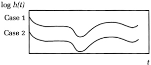
What’s important about this equation is that λ₀(t) cancels out of the numerator and denominator. As a result, the ratio of the hazards is constant over time. If we graph the log hazards for any two individuals, the proportional hazards property implies that the hazard functions should be strictly parallel, as in Figure 5.1.