
Tied Data
The formula for the partial likelihood in equation (5.10) is valid only for data in which no two events occur at the same time. It’s quite common for data to contain tied event times, however, so we need an alternative formula to handle those situations. Most partial likelihood programs use a technique called Breslow’s approximation, which works well when ties are relatively few. But when data are heavily tied, the approximation can be quite poor (Farewell and Prentice 1980; Hsieh 1995). Although PROC PHREG uses Breslow’s approximation as the default, it is unique in providing a somewhat better approximation proposed by Efron (1977) as well as two exact methods.
This section explains the background, rationale, and implementation of these alternative methods for handling ties. Since this issue is both new and confusing, I’m going to discuss it at considerable length. Those who just want the bottom line can skip to the end of the section where I summarize the practical implications. Because the formulas can get rather complicated, I won’t go into all the mathematical details. But I will try to provide some intuitive understanding of why there are different approaches and the basic logic of each one.
To illustrate the problem and the various solutions, let’s turn again to the recidivism data. As output 5.6 shows, these data include a substantial number of tied survival times (weeks to first arrest). For weeks 1 through 7, there is only one arrest in each week. For these seven events, the partial likelihood terms are constructed exactly as described in the section Partial Likelihood: Mathematical and Computational Details. Five arrests occurred in week 8, however, so the construction of L8 requires a different method. Two alternative approaches have been proposed for the construction of the likelihood for tied event times; these are specified in PROC PHREG by TIES=EXACT or TIES=DISCRETE as options in the MODEL statement. This terminology is somewhat misleading because both methods give exact likelihoods; the difference is that the EXACT method assumes that there is a true but unknown ordering for the tied event times (i.e., time is continuous), while the DISCRETE method assumes that the events really occurred at exactly the same time.
Output 5.6. Week of First Arrest for Recidivism Data
Cumulative Cumulative WEEK Frequency Percent Frequency Percent -------------------------------------------------- 1 1 0.2 1 0.2 2 1 0.2 2 0.5 3 1 0.2 3 0.7 4 1 0.2 4 0.9 5 1 0.2 5 1.2 6 1 0.2 6 1.4 7 1 0.2 7 1.6 8 5 1.2 12 2.8 9 2 0.5 14 3.2 10 1 0.2 15 3.5 11 2 0.5 17 3.9 12 2 0.5 19 4.4 13 1 0.2 20 4.6 14 3 0.7 23 5.3 15 2 0.5 25 5.8 16 2 0.5 27 6.2 17 3 0.7 30 6.9 18 3 0.7 33 7.6 19 2 0.5 35 8.1 20 5 1.2 40 9.3 21 2 0.5 42 9.7 22 1 0.2 43 10.0 23 1 0.2 44 10.2 24 4 0.9 48 11.1 25 3 0.7 51 11.8 26 3 0.7 54 12.5 27 2 0.5 56 13.0 28 2 0.5 58 13.4 30 2 0.5 60 13.9 31 1 0.2 61 14.1 32 2 0.5 63 14.6 33 2 0.5 65 15.0 34 2 0.5 67 15.5 35 4 0.9 71 16.4 36 3 0.7 74 17.1 37 4 0.9 78 18.1 38 1 0.2 79 18.3 39 2 0.5 81 18.8 40 4 0.9 85 19.7 42 2 0.5 87 20.1 43 4 0.9 91 21.1 44 2 0.5 93 21.5 45 2 0.5 95 22.0 46 4 0.9 99 22.9 47 1 0.2 100 23.1 48 2 0.5 102 23.6 49 5 1.2 107 24.8 50 3 0.7 110 25.5 52 322 74.5 432 100.0 |
The EXACT Method
Let’s begin with the EXACT method since its underlying model is probably more plausible for most applications. Since arrests can occur at any point in time, it’s reasonable to suppose that ties are merely the result of imprecise measurement of time and that there is a true time ordering for the five arrests that occurred in week 8. If we knew that ordering, we could construct the partial likelihood in the usual way. In the absence of any knowledge of that ordering, however, we have to consider all the possibilities. With five events, there are 5! = 120 different possible orderings. Let’s denote each of those possibilities by Ai, where i = 1, ..., 120. What we want is the probability of the union of those possibilities, that is, Pr(A1 or A2 or ... or A120). Now, a fundamental law of probability theory is that the probability of the union of a set of mutually exclusive events is just the sum of the probabilities for each of the events. Therefore, we can write
Equation 5.12
![]()
Each of these 120 probabilities is just a standard partial likelihood. Suppose, for example, that we arbitrarily label the five arrests at time 8 with the numbers 8, 9, 10, 11, and 12, and suppose further that A1 denotes the ordering {8, 9, 10, 11, 12}. Then
On the other hand, if A2 denotes the ordering {9, 8, 10, 11, 12}, we have
We continue in this way for the other 118 possible orderings. Then L8 is obtained by adding all the probabilities together.
The situation is much simpler for week 9 because only two arrests occurred, giving us two possible orderings. For L9, then, we have
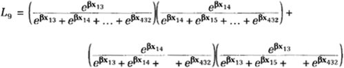
where the numbers 13 and 14 are arbitrarily assigned to the two events. When we get to week 10, there’s only one event so we’re back to the standard partial likelihood formula:
![]()
It’s difficult to write a general formula for the exact likelihood with tied data because the notation becomes very cumbersome. For one version of a general formula, see Kalbfleisch and Prentice (1980). Be forewarned that the formula in the official PROC PHREG documentation bears no resemblance to that given by Kalbfleisch and Prentice or to the explanation given here. That’s because it’s based on a re-expression of the formula in terms of a definite integral, which facilitates computation (DeLong, Guirguis, and So 1994).
It should be obvious, by this point, that computation of the exact likelihood can be a daunting task. With just five tied survival times, we have seen that one portion of the partial likelihood increased from 1 term to 120 terms. If 10 events occur at the same time, there are over three million possible orderings to evaluate. Until recently, statisticians abandoned all hope that such computations might be practical (which is why no other programs calculate the exact likelihood). What makes it possible now is the development of an integral representation of the likelihood, which is much easier to evaluate numerically. Even with this innovation, however, computation of the exact likelihood when large numbers of events occur at the same time can take an enormous amount of computing time.
Early recognition of these computational difficulties led to the development of approximations. The most popular of these is widely attributed to Breslow (1974), but it was first proposed by Peto (1972). This is the default in PROC PHREG, and it is nearly universal in other programs. Efron (1977) proposed an alternative approximation that is also available in PROC PHREG. The results we saw earlier in Output 5.1 for the recidivism data were obtained with the Breslow approximation.
To use the EXACT method, we specify
proc phreg data=recid;
   model week*arrest(0)=fin age race wexp mar paro prio
         / ties=exact;
run;
This PROC step produces the results in Output 5.7. Comparing this with Output 5.1, it’s apparent that the Breslow approximation works well in this case. The coefficients are generally the same to at least two (and sometimes three) decimal places. The test statistics all yield the same conclusions.
Output 5.7. Recidivism Results Using the EXACT Method
                         The PHREG Procedure
               Testing Global Null Hypothesis: BETA=0

              Without       With
Criterion   Covariates   Covariates   Model Chi-Square

-2 LOG L      1227.506     1194.239     33.266 with 7 DF (p=0.0001)
Score             .            .        33.529 with 7 DF (p=0.0001)
Wald              .            .        32.112 with 7 DF (p=0.0001)

               Analysis of Maximum Likelihood Estimates

                 Parameter   Standard    Wald       Pr >        Risk
  Variable DF     Estimate     Error  Chi-Square Chi-Square    Ratio

  FIN       1    -0.379427    0.19138    3.93061     0.0474    0.684
  AGE       1    -0.057438    0.02200    6.81663     0.0090    0.944
  RACE      1     0.313906    0.30800    1.03875     0.3081    1.369
  WEXP      1    -0.149793    0.21223    0.49817     0.4803    0.861
  MAR       1    -0.433705    0.38187    1.28990     0.2561    0.648
  PARO      1    -0.084873    0.19576    0.18798     0.6646    0.919
PRIO 1 0.091500 0.02865 10.20021 0.0014 1.096 |
Output 5.8 shows the results from using Efron’s approximation (invoked by using TIES=EFRON). If Breslow’s approximation is good, this one is superb. Nearly all the numbers are the same to four decimal places. In all cases where I’ve tried the two approximations, Efron’s approximation gave results that were much closer to the exact results than Breslow’s approximation. This improvement comes with only a trivial increase in computation time. For the recidivism data, Breslow’s approximation took five seconds and Efron’s formula took six seconds on a 486 DOS machine. By contrast, the EXACT method took 18 seconds.
Output 5.8. Recidivism Results Using Efron’s Approximation
               Testing Global Null Hypothesis: BETA=0

              Without       With
Criterion   Covariates   Covariates   Model Chi-Square

-2 LOG L      1350.761     1317.495     33.266 with 7 DF (p=0.0001)
Score             .            .        33.529 with 7 DF (p=0.0001)
Wald              .            .        32.113 with 7 DF (p=0.0001)
               Analysis of Maximum Likelihood Estimates

                 Parameter   Standard    Wald       Pr >        Risk
  Variable DF     Estimate     Error  Chi-Square Chi-Square    Ratio

  FIN       1    -0.379422    0.19138    3.93056     0.0474    0.684
  AGE       1    -0.057438    0.02200    6.81664     0.0090    0.944
  RACE      1     0.313900    0.30799    1.03873     0.3081    1.369
  WEXP      1    -0.149796    0.21222    0.49821     0.4803    0.861
  MAR       1    -0.433704    0.38187    1.28991     0.2561    0.648
  PARO      1    -0.084871    0.19576    0.18797     0.6646    0.919
PRIO 1 0.091497 0.02865 10.20021 0.0014 1.096 |
If the approximations are so good, why do we need the computationally intensive EXACT method? Farewell and Prentice (1980) showed that the Breslow approximation deteriorates as the number of ties at a particular point in time becomes a large proportion of the number of cases at risk. For the recidivism data in Output 5.6, the number of tied survival times at any given time point is never larger than 2 percent of the number at risk, so it’s not surprising that the approximations work well.
Now let’s look at an example where the conditions are less favorable. The data consist of 100 simulated job durations, measured from the year of entry into the job until the year that the employee quit. Durations after the fifth year are censored. If the employee was fired before the fifth year, the duration is censored at the end of the last full year in which the employee was working. We know only the year in which the employee quit, so the survival times have values of 1, 2, 3, 4, or 5.
Here’s a simple life table for these data:
| Duration | Number Ouit | Number Censored | Number At Risk | Quit/At Risk |
|---|---|---|---|---|
| 1 | 22 | 7 | 100 | .22 |
| 2 | 18 | 3 | 71 | .25 |
| 3 | 16 | 4 | 50 | .32 |
| 4 | 8 | 1 | 30 | .27 |
| 5 | 4 | 17 | 21 | .19 |
The number at risk at each duration is equal to the total number of cases (100) minus the number who quit or were censored at previous durations. Looking at the last column, we see that the ratio of the number quitting to the number at risk is substantial at each of the five points in time. Three covariates were measured at the beginning of the job: years of schooling (ED), salary in thousands of dollars (SALARY), and the prestige of the occupation (PRESTIGE) measured on a scale from 1 to 100.
Output 5.9 displays selected results from using PROC PHREG with the three different methods for handling ties. Breslow’s method yields coefficient estimates that are about one-third smaller in magnitude than those using the EXACT method, while the p-values (for testing the hypothesis that each coefficient is 0) are substantially higher. In fact, the p-value for the SALARY variable is above the .05 level for Breslow’s method, but it is only .01 for the EXACT method. Efron’s method produces coefficients that are about midway between the other two methods, but the p-values are much closer to those of the EXACT method. Clearly, the Breslow approximation is unacceptable for this application. Efron’s approximation is not bad for drawing qualitative conclusions, but there is an appreciable loss of accuracy in estimating the magnitudes of the coefficients. With regard to computing time, both approximate methods took 3 seconds on a 486 DOS machine. The EXACT method took 24 seconds.
Output 5.9. Results for Job Duration Data: Three Methods for Handling Ties
Ties Handling: BRESLOW

                 Parameter   Standard    Wald       Pr >        Risk
  Variable DF     Estimate     Error  Chi-Square Chi-Square    Ratio

  ED        1     0.116453    0.05918    3.87257     0.0491    1.124
  PRESTIGE  1    -0.064278    0.00959   44.93725     0.0001    0.938
  SALARY    1    -0.014957    0.00792    3.56573     0.0590    0.985


Ties Handling: EFRON

                 Parameter   Standard    Wald       Pr >        Risk
  Variable DF     Estimate     Error  Chi-Square Chi-Square    Ratio

  ED        1     0.144044    0.05954    5.85271     0.0156    1.155
  PRESTIGE  1    -0.079807    0.00996   64.20009     0.0001    0.923
  SALARY    1    -0.020159    0.00830    5.90363     0.0151    0.980


Ties Handling: EXACT

                 Parameter   Standard    Wald       Pr >        Risk
  Variable DF     Estimate     Error  Chi-Square Chi-Square    Ratio

  ED        1     0.164332    0.06380    6.63419     0.0100    1.179
  PRESTIGE  1    -0.092019    0.01240   55.10969     0.0001    0.912
SALARY 1 -0.022545 0.00884 6.50490 0.0108 0.978 |
The DISCRETE Method
The DISCRETE option in PROC PHREG is also an exact method, but one based on a fundamentally different model. In fact, it is not a proportional hazards model at all. The model does fall within the framework of Cox regression, however, since it was proposed by Cox in his original 1972 paper and since the estimation method is a form of partial likelihood. Unlike the EXACT model, which assumes that ties are merely the result of imprecise measurement of time, the DISCRETE model assumes that time is really discrete. When two or more events appear to happen at the same time, there is no underlying ordering—they really happen at the same time.
While most applications of survival analysis involve events that can occur at any moment on the time continuum, there are definitely some events that are best treated as if time were discrete. If the event of interest is a change in the political party occupying the U.S. presidency, that can only occur once every four years. Or suppose the aim is to predict how many months it takes before a new homeowner misses a mortgage payment. Because payments are only due at monthly intervals, a discrete-time model is the natural way to go.
Cox’s model for discrete-time data can be described as follows. The time variable t can only take on integer values. Let Pit be the conditional probability that individual i has an event at time t, given that an event has not already occurred to that individual. This probability is sometimes called a discrete-time hazard. The model says that Pit is related to the covariates by a logit-regression equation:
![]()
The expression on the left side of the equation is the logit or log-odds of Pit. On the right side, we have a linear function of the covariates, plus a term αt that plays the same role as α(t) in expression (5.2) for the proportional hazards model. αt is just a set of constants—one for each time point—that can vary arbitrarily from one time point to another.
This model can be described as a proportional odds model, although that term has a different meaning here than it did in Chapter 4 (see the section The Log-Logistic Model). The odds that individual i has an event at time t (given that i did not already have an event) is just Oit = Pit/(1 - Pit). The model implies that ratio of the odds for any two individuals Oit/Ojt does not depend on time (although it may vary with the covariates).
How can we estimate this model? In Chapter 7, “Analysis of Tied or Discrete Data with the LOGISTIC, PROBIT, and GENMOD Procedures,” we will see how to estimate it using standard maximum likelihood methods that yield estimates of both the β coefficients and the αts. Using partial likelihood, however, we can treat the αts as nuisance parameters and estimate only the βs. If there are J unique times at which events occur, there will be J terms in the partial likelihood function:
![]()
where Lj is the partial likelihood of the jth event. Thus, for the job duration data, there are only five terms in the partial likelihood function. But each of those five terms is colossal. Here’s why:
At time 1, there were 22 people with events out of 100 who were at risk. To get L1 we ask the question: given that 22 events occurred, what is the probability that they occurred to these particular 22 people rather than to some different set of 22 people from among the 100 at risk? How many different ways are there of selecting 22 people from among a set of 100? A lot! Specifically, 7.3321 × 10²¹. Let’s call that number Q, and let q be a running index from 1 to Q, with q = 1 denoting the set that actually experienced the events. For a given set q, let ψq be the product of the odds for all the individuals in that set. Thus, if the individuals who actually experienced events are labeled i = 1 to 22, we have
![]()
We can then write
![]()
This is a simple expression, but there are trillions of terms being summed in the denominator. Fortunately, there is a recursive algorithm that makes it practical, even with substantial numbers of ties (Gail et al. 1981). Still, doing this with a large data set with many ties can take a great deal of computer time.
For the job duration data, the DISCRETE method takes only 11 seconds of computer time on a 486 DOS machine as compared with 3 seconds each for the Breslow and Efron approximations and 24 seconds for the EXACT method. But does the discrete-time model make sense for these data? For most jobs it’s possible to quit at any point in time, suggesting that the model might not be appropriate. Remember, however, that these are simulated data. Since the simulation is actually based on a discrete-time model, it makes perfectly good sense in this case. Output 5.10 displays the results. Comparing these with the results for the EXACT method in Output 5.9, we see that the chi-square statistics and the p-values are similar. However, the coefficients for the DISCRETE method are about one-third larger for ED and PRESTIGE and about 15 percent larger for SALARY. This discrepancy is due largely to the fact that completely different models are being estimated, a hazard model and a logit model. The logit coefficients will usually be larger. For the logit model, 100(eβ – 1) gives the percent change in the odds that an event will occur for a one-unit increase in the covariate. Thus, each additional year of schooling increases the odds of quitting a job by 100(e.219–1) = 24 percent.
Output 5.10. Job Duration Results Using the DISCRETE Method
Ties Handling: DISCRETE

               Analysis of Maximum Likelihood Estimates

                 Parameter   Standard    Wald       Pr >         Risk
  Variable DF     Estimate     Error  Chi-Square Chi-Square     Ratio

  ED        1     0.219378    0.08480    6.69295     0.0097     1.245
  PRESTIGE  1    -0.120474    0.01776   46.02220     0.0001     0.886
SALARY 1 -0.026108 0.01020 6.55603 0.0105 0.974 |
Comparison of Methods
Though the job duration coefficients differ for the two exact methods, they are at least in the same ballpark. More generally, it has been shown that if ties result from grouping continuous time data into intervals, the logit model converges to the proportional hazards model as the interval length gets smaller (Thompson 1977). When there are no ties, the partial likelihoods for all four methods (the two exact methods and the two approximations) reduce to the same formula, although PROC PHREG is still slightly faster with the Breslow method.
The examples we’ve seen so far have been small enough, both in number of observations and numbers of ties, that the computing times for the two exact methods were quite tolerable. Before concluding, let’s see what happens as those data sets get larger. I took the 100 observations in the job duration data set and duplicated them to produce data sets of size 200, 400, 800, 1000, and 1200. The models were run on a Power Macintosh 7100/80 using a preproduction version of Release 6.10 SAS/STAT software. Here are the elapsed times, in seconds, for the four methods and seven sample sizes:
| 100 | 200 | 400 | 600 | 800 | 1000 | 1200 | |
|---|---|---|---|---|---|---|---|
| BRESLOW | 3 | 3 | 3 | 3 | 4 | 5 | 5 |
| EFRON | 3 | 3 | 3 | 3 | 4 | 5 | 5 |
| EXACT | 4 | 6 | 18 | 38 | 70 | 129 | 204 |
| DISCRETE | 3 | 4 | 6 | 9 | 12 | 19 | 26 |
For the two approximate methods, computing time hardly increased at all with the sample size, and the methods had identical times in every case. For the EXACT method, on the other hand, computing time went up much more rapidly than the sample size. Doubling the sample size from 600 to 1200 increased the time by a factor of over five times. I also tried the EXACT method with an additional doubling to 2400 observations, which increased time to 20 minutes, a factor of nearly six times. Computing time for the DISCRETE method rose at about the same rate as the number of observations. On the other hand, the DISCRETE method produced a floating-point divide error for anything over 1200 cases. According to a SAS Note, this bug occurs in Release 6.10 whenever the number of ties at any one time point exceeds about 250 (the exact number dependent on the operating system).
What we’ve learned about the handling of ties can be summarized in six points:
When there are no ties, all four options in PROC PHREG give identical results.
When there are few ties, it makes little difference which method is used. But since computing times will also be comparable, you might as well use one of the exact methods.
When the number of ties is large, relative to the number at risk, the approximate methods tend to yield coefficients that are biased toward 0.
Both the EXACT and DISCRETE methods produce exact results (i.e., true partial likelihood estimates), but the EXACT method assumes that ties arise from grouping continuous, untied data, while the DISCRETE method assumes that events really occur at the same, discrete times. The choice should be based on substantive grounds, although qualitative results will usually be similar.
Both of the exact methods need a substantial amount of computer time for large data sets containing many ties. This is especially true for the EXACT method where doubling the sample size increases computing time by at least a factor of 5.
If the exact methods are too time-consuming, use the Efron approximation, at least for model exploration. It’s nearly always better than the Breslow method, with virtually no increase in computer time.