
5
Reliable Systems on a Spatial Scale
Simplicity is prerequisite for reliability.
5.1 Principle 2
A system is a region where EEIS are intended to serve. On a spatial scale, a system can be classified as residential, community, city, country, or global level. Reliability is defined as the duration of an EEIS to function normally and provide the required service to protect human health and the environments under normal conditions. Reliability usually is measured by the time period during which the system will not fail. Therefore, it can be quantified as the time from starting service to failure of the system. EEIS should be designed in such a way that their reliability is quantified with known uncertainty and sensitivity on different spatial scales. To reduce probability of failure is to design EEIS as simple as possible because propagation of failure increases with increasing components.
Reliability on spatial scales must be quantified in designing EEIS such as WTPs, WWTPs, and GIs. Local geography, resource, economy, and culture could also be weighted to increase reliability of EEIS. For a household, if the land is large enough, on‐site WWT processes such as septic tanks and constructed wetlands could be the most economical way to achieve regenerative design. For communities of population greater than 1000 PE, energy‐neutral design may be more realistic. For large cities, if energy‐neutral design cannot be achieved, designers should target maximum reuse of materials and energy to reduce the FP on water, energy, and nutrients. In general, decentralized WWT is more suitable for rural areas than metropolitan cities. New urban communities and cities have the opportunity to design and build source‐separating systems optimized for cost‐effective resource recovery due to established technologies and design strategies. EEIS should be designed to support sustainable industries, agriculture, and social institutions. Engineers should design EEIS adapted to local geographical conditions, because local resources and geographical settings significantly influence the availability of water, energy, and nutrients. For example, in hilly settings, WTP and WRRF should be sited on a slope from 1 to 3% when gravity flow is used to save energy needed for pumping. For WRRF, reliability is affected by the variability of system performance under normal operation and impact of mechanical failure. For WTP, two components determining the system reliability are the probability of being online and the number of parallel treatment units (AWWA, 2012). To achieve reliability at different spatial scales, following design strategies are recommended:
- To achieve reliability, design philosophy should switch from fit for all to fit for purpose.
- Economy of scale should be quantified in terms of unit cost on individual, household, community, city, state, and country levels.
- Zero discharge and energy‐independent residential house should be designed when sufficient land or space is available.
- Green infrastructure (GI) should be implemented as much as possible on household, community, city, state, and country levels to prevent nonpoint pollution.
- Laboratory, pilot, and full‐scale testing should be validated with quantified uncertainty to increase the reliability of EEIS. Laboratory‐scale data could be used to design the full‐scale system if kinetics and mechanisms are fully understood and validated through computer simulation.
- Separated management of blue, green, gray, brown, and black water could increase reliability on a specific spatial scale.
- Decentralized WRRF could increase reliability of water utility for small to medium size cities due to its approximate to irrigation and other water reuse demands.
In designing an EEIS, basic research on molecular reaction, applied research on materials and components, and the development of devices and products should consider the life cycle impact of the EEIS on the environments. Figure 5.1 shows that basic and applied research, product development, and manufacturing are corresponding to molecules, materials, components, and products. Life cycle assessment should be used to quantify and minimize the footprints on the environments at each stage. Since all the stages interact with environments, increasing reliability should not increase environmental impacts.

Figure 5.1 Schematic of sustainable environmental engineering system development.
5.1.1 Central Versus Decentralized WWTP
Sedlak (2014) considered that water and wastewater engineering have went through four stages: (i) transportation of water for drinking and irrigation in the Roman Empire 2000 years ago until 1800, (ii) water treatment and the collection of wastewater and discharge into nature in England until 1900, (iii) centralized wastewater treatment plants from 1900 to today, and (iv) decentralized wastewater treatment that may offer ecological and economic benefits from now on as the fourth stage. Indeed, aging EEIS such as WWTPs causes great problems due to increased population, infiltration, and inflow in sewer system. For example, from January 2007 to May 2013, Miami‐Dade County reported 211 sewer overflows totaling in excess of 51 million gallons, including at least 29 million gallons of raw sewage. In June 2013, the Environmental Protection Agency (EPA) and the state of Florida imposed a fine of $978 000 on the Miami‐Dade County for wastewater violations. The county has to sell a $13.6 billion bond to finance the required repairs of three WWTPs, ending ocean outfalls, upgrading pump stations, and constructing deep wells for the injection of treated wastewater. While the county has made progress toward improving operations since the penalty was issued, many proposed projects are not necessarily sustainable in terms of increasing system reliability. For example, $4 billion is proposed to design and construct two deep wells to dispose treated effluent after high level chlorination at the North and Central WWTPs. Many stakeholders and county commissioners are expressing their concerns for wasting tax payers’ money. Indeed, to increase reliability of the system, innovative technologies have to be assessed to reclaim the effluent for reuse and avoid the costly deep well injection.
In developing countries, decentralized wastewater treatment appears to be even more important. Rudimentary sanitation facilities such as stand‐alone septic tanks, composting or pit toilets, may be one of the best solutions for low‐income areas. However, the potential of contaminating the ground or surface water makes it necessary to employ decentralized WWTP, because conventional on‐site treatment has proved to be of low community acceptance while conventional sewage is too costly. Oxidation ponds, constructed wetlands, sand filters, and biological disks could be effectively applied in small communities as decentralized treatment technologies. A decentralized wastewater management system is defined as a wastewater treatment system that collects wastewater from the source, conveys to a treatment system, and disperses the water near the point of origin. It includes treatment facilities in rural, satellite, cluster, on‐site, and small WWTPs. Small WWTPs refer plants with flow rates ranging from 1 000 to 50 000 GPD. There are also privately owned WWTPs such as mobile home parks, camp sites, recreational facilities, apartments, schools, and privately owned public facilities such as condominiums, shopping centers, and parks. Major advantages of these systems include the protection of public health and the environment, cost effectiveness, recharging of local aquifers, and the provision of water close to wastewater generation. Therefore, they are appropriate for low‐density communities with varying site conditions and are especially suitable for ecologically sensitive areas. Small WWTP systems can be optimized to achieve low cost and high performance with several criteria. They should be easy to be constructed using low‐precision construction techniques, minimize moving parts, operate without electricity, provide feedback on the performance of every step of the treatment process, operate without complicated calculations, and use chemical dosages that can be set directly by a few persons.
5.1.2 Best Practice for Small WWTPs
US EPA recommends the following procedure as the best practice to increase the reliability of small WWTPs:
- Preparing an asset inventory and system maps.
- Developing a condition assessment and rating system.
- Assessing remaining useful life by consulting projected‐useful‐life tables or decay curves.
- Determining asset values and replacement costs.
- Analyzing current and anticipated customer demand and satisfaction with the system.
- Understanding current and anticipated regulatory requirements.
- Writing system’s performance targets.
- Using level of service standards to track system performance over time.
- Conducting a failure analysis (root cause analysis, failure mode analysis).
- Determining the probability of failure and listing assets by failure type.
- Analyzing failure risk and consequences.
- Reviewing and updating system’s vulnerability assessment.
Financing assets for rehabilitation, repair, and replacement through borrowing or other financial assistance should be analyzed in asset management plan (long term). The asset management program should assess performance, evaluate progress, adopt new best practices, and take action based on review results to ensure that assets are managed to ensure reliable EEISs.
5.2 Integrated System Approach
5.2.1 The EPA Tools
There are many tools available to facilitate the decision‐making process of different treatment options. Table 5.1 lists analysis tools that the US EPA provided to design an integrated system by selecting.
Table 5.1 Analysis tools.
| Tools | Description |
| Check Up Program for Small Systems (CUPSS) | This EPA‐developed software provides a simple comprehensive approach to asset management for small water and wastewater utilities in an easy‐to‐use, no‐cost package |
| Financing Alternatives Comparison Tool (FACT) | A financial analysis tool developed by EPA to identify the most cost‐effective method to fund a wastewater or drinking water management project |
| The Wastewater Information System Tool (TWIST) | This computer‐based tool allows state and local health departments to inventory and manage small wastewater treatment systems by tracking information on residences and facilities served, permits, site evaluations, types of systems, inspections, and complaints in their jurisdictions |
| Water and Wastewater Treatment Technologies Appropriate for Reuse (WAWTTAR) | This software identifies appropriate water and wastewater treatment options. It estimates local performance and costs associated with each system based on available material and manpower resources |
Operations and maintenance (O&M), personnel, and the capital budget account for an estimated 85% of a typical water system’s expenses. Asset management enables a system to determine the lowest cost options for providing the highest level of reliable service over time. The work by O&M crew should be optimized on what are they doing, where they are doing it, and why the tasks have to be performed as listed by the US EPA in Table 5.2.
Table 5.2 Five core questions for SWWTPs.
| Step | Action |
| 1 | What is the current state of my system’s assets? |
| 2 | What is my required “sustainable” level of service? |
| 3 | Which assets are critical to sustained performance? |
| 4 | What are my minimum life cycle costs? |
| 5 | What is my best long‐term funding strategy? |
5.2.2 Integrated Engineering Design Example
Figure 5.2 Components of a conventional on‐site wastewater treatment and reuse system. Table 5.3 Daily water consumption for standard domestic appliances. Figure 5.3 Cross section of a single‐compartment septic tank. Table 5.4 Daily water consumption for water‐efficient domestic appliances. Table 5.5 Comparing the costs and water consumption of standard and water‐efficient appliances. Table 5.6 Comparing the capital and running costs of the water treatment and reuse systems. Figure 5.4 Comparison of the capital costs of components. Figure 5.5 Comparison of the operation costs of components. Table 5.7 Comparing the total cost of conventional and IED systems over 20 years. Figure 5.6 Comparison of the total cost of the conventional and integrated engineering design systems over 20 years.
Waste source
Allowance (l/person/day)
Toilet
50
Bath and shower
50
Handbasin tap
10
Kitchen
10
Tap
7
Dishwasher
3
Laundry
30
Tap
5
Washing machine
25
Total
150
Waste source
Allowance (l/person/day)
Toilet
33
Bath and shower
19
Handbasin tap
1
Kitchen
3
Tap
1
Dishwasher
2
Laundry
11
Tap
1
Washing machine
10
Total
64
Water‐consuming appliances
Capital costs (not installed)
Water consumption
Running costs (water only)
Standard appliances
$2650
273 kl/year
$129/year
Toilet
$300
Shower head
$50
Taps
$800
Dishwasher
$700
Washing machine
$800
Water‐efficient appliances
$3380
116 kl/year
$55/year
Toilet
$300
Shower head
$80
Taps
$1000
Dishwasher
$1000
Washing machine
$1000
Water treatment and reuse system
Capital costs (installed)
Running costs
Conventional solution
$10 836
$640/year
Septic system
$6 500
$240/year
Slow sand filter system
$1 500
$400/year
Subsurface drip irrigation system
$2 836
WDS solution
$10 701
$367/year
Biolytix system
$8 829
$367/year
Subsurface drip irrigation system
$1 872

Solution
Capital costs
O/M costs
20‐year cost
20‐year water consumption
Conventional
$13 486 + $3 630 in 10 years
$769/year
$25 741
5460 kl
Whole system design
$14 081
$422/year
$18 311
2320 kl
5.3 Scale‐up of Laboratory or Pilot Design to Full‐scale Plant
Innovative technologies in EEIS design start from laboratory research. Therefore, laboratory data are the major source for scaling up to pilot and full scale. For example, to ensure the reliability of a UV disinfection system to achieve a specific inactivation level of log inactivation (log I), the US EPA requires utilities to validate their UV processes so that the credit of a specific log I can be granted.
5.3.1 Minimum Requirements for Validation Testing
Reliability must be proven according to the US EPA protocol of UV disinfection from laboratory data to the full‐scale reactor. In addition, uncertainty associated with the scale‐up must be quantified so that the system can perform as expected to earn the US EPA disinfection credit under different flow rate or water quality such as the transmittance of water. Although UV sensors can measure the intensity of UV light, they cannot measure the dose delivered to the microorganisms as they pass through the reactor at different trajectories. Therefore, to receive treatment credit for inactivating Cryptosporidium, Giardia, or viruses using UV light, the LT2ESWTR requires water systems to use UV reactors that have undergone validation testing. Table 5.8 summarizes the regulatory requirements for all LT2ESWTR requirements related to UV disinfection, including minimum dose, validation, monitoring, and reporting requirements.
Table 5.8 Summary of LT2ESWTR validation requirements.
| Requirement | Conditions |
| Validated operating conditions must include |
|
| Validation testing must include |
|
| Validation testing must account for |
|
5.3.1.1 Collimated Beam Test
Collimated beam test typically has the following steps (US EPA, 2006):
- The microbe of interest is cultured under controlled and reproducible laboratory conditions.
- This culture is then prepared for testing, again under controlled and reproducible conditions: (i) there is a known concentration and/or distribution of the cultured pathogen, and (ii) the medium in which the culture is to be presented is of a known UVT.
- The culture is then exposed to a known UV intensity, of known wavelength, for a fixed period of time, delivering a known UV dose to the known area of the presentation plate; hence dose and intensity are measured per cm2 (area) rather than cm3 (volume), which is referred as a collimated beam apparatus.
- The exposed content is recultured to see how many of the microbes survived.
- This procedure is replicated many times at systematically increasing doses to build a dose–response curve. This curve enables the log survival (and by inference, log reduction) for the microbe of interest to be determined at any given UV dose.
- After the various dose–response curves have been constructed in the laboratory, these curves would be applied to test an actual UV system to validate the actual Log I. The important thing is that the microbes used to test the UV system are cultured (albeit in much higher volumes) under exactly the same conditions as were used in the laboratory. This microbe culture is presented to the UV system mixed with the water of known UVT and tested over the range of UVTs and flow rates of interest.
- A sample of the water is taken at the entry and exit of the UV system and recultured to quantify the reduction of the microbe.
- Using the observed log reduction of the microbe and comparing it with the microbe’s dose–response curve, the UV dose delivered can be determined. This UV dose is termed the reduction equivalent dose (RED).
US EPA (2006) recommends test procedure using a challenge microbe such as MS2 for health, safety, and repeatability. To validate the full‐scale UV reactor, biodosimetric‐tested RED dose results from the real‐life tests with actual microbes should be used to measure the reactor performance using the following three steps:
- Step 1: Conduct experimental tests using a challenge microorganism. A challenge microorganism whose sensitivity to UV light is similar to the target pathogen is recommended in all experiments by US EPA (2006). However, it introduces uncertainty into the testing results. This uncertainty is accounted for by applying a validation factor (VF) as described in step 3. Two types of experimental tests can be used for UV reactor validation: (i) bench‐scale testing using a collimated beam apparatus and (ii) full‐scale reactor testing.
Bench‐scale testing using a collimated beam apparatus. Collimated beam testing characterizes the UV dose–response relationship of the challenge microorganism. UV light is directed through a collimating tube to dose a sample of challenge microorganisms of a known concentration. After a specified exposure time, the sample is analyzed to determine the log inactivation (where log inactivation in this situation equals the log concentration prior to UV light exposure minus the log concentration after UV light exposure) as a function of UV dose. The UV dose delivered to the microorganisms is calculated based on the UV intensity, exposure time, and other experimental factors. Collimated beam tests are performed at a range of doses to generate a UV dose–response curve for the specific challenge microorganism. The functional forms of the equations for UV dose–response curves can vary depending on the results. EPA provided guidance on developing UV dose–response curves (US EPA, 2006). A quadratic UV dose–response equation can be used as follows:
(5.1)
The coefficients A and B would be solved for using the collimated beam testing data by Example 5.2 using Matlab. UVT is typically reported at 254 nm because UV manufacturers, WTPs and WWTPs widely use A254.
Full‐scale reactor testing. The challenge microorganisms are injected upstream of the UV reactor. Samples are analyzed to determine the log inactivation at the test conditions of flow rate, UVT, lamp status, and UV intensity as measured by UV sensors. Full‐scale reactor testing can be performed on‐site at a water or a wastewater treatment plant or off‐site at a validation test center.
- Step 2: Estimate the RED. The results from the two experimental tests in step 1 are combined. The log inactivation of the challenge microorganism measured during the full‐scale testing is entered into the UV dose–response equation (if the relationship is quadratic) to calculate the RED of the reactor. Another way to conceptualize this step is to consider the RED to be “back calculated” using the field‐measured log inactivation as the input variable. This approach is the opposite of most applications in which UV dose is the independent variable and log inactivation is the dependent variable. RED values are always specific to challenge microorganism used during experimental testing and the validation test conditions during full‐scale reactor tests (flow rate, UVT, lamp status, and UV intensity as measured by the UV sensor).
- Step 3: Adjust for uncertainty to calculate the validated dose. RED is divided by a VF to produce the validated dose. The VF accounts for biases associated with using a challenge microorganism instead of the target pathogen, and experimental uncertainty provides a detailed description of how the VF is derived. The validated dose is associated with the validation test conditions of flow rate, lamp status, UV intensity as measured by a UV sensor, and, in some cases, UVT. The validated dose is compared with the required dose to determine the inactivation credit for the target pathogen.
5.3.2 Correlation of UV Sensitivity of Different Challenge Microorganisms with Target Microorganisms
Male‐specific‐2 bacteriophage (MS2) and Bacillus subtilis spores have historically been used for validation testing to receive treatment credit for Cryptosporidium and Giardia. Of importance is how much the UV sensitivity of each microorganism is related to the target microorganisms. The UV sensitivity of some commonly used and some candidate bioassay microorganisms is shown in Table 5.9.
Table 5.9 UV sensitivity of challenge microorganisms (US EPA, 2006).
| Microorganism | Reported delivered UV dose(mJ/cm2) to achieve indicated log inactivation | Reference | |||
| 1‐log | 2‐log | 3‐log | 4‐log | ||
| Bacillus subtilis | 28 | 39 | 50 | 62 | Sommer et al. (1998a) |
| MS2 phage | 16 | 34 | 52 | 71 | Wilson et al. (1992 |
| Qß phage | 10.9 | 22.5 | 34.6 | 47.6 | Mackey et al.(2006) |
| PRD‐1 phage | 9.9 | 17 | 24 | 30 | Mengand Gerba (1996) |
| B40‐8 phage | 12 | 18 | 23 | 28 | Sommer et al. (1998b) |
| φx174 phage | 2.2 | 5.3 | 7.3 | 11 | Sommer et al. (1998b) |
| E. coli | 3.0 | 4.8 | 6.7 | 8.4 | Chang et al. (1985) |
| T7 | 3.6 | 7.5 | 11.8 | 16.6 | Mackey et al. (2006) |
| T1 | ~5 | ~10 | ~15 | ~20 | Wright (2006) |
Since the UVT of water has to be monitored during operations, it is critical to validate the UV reactor to confirm dose delivery.
Figure 5.7 Dose–response standard relationship by NWRI. The sampling points for microorganisms should be placed far enough from the UV reactor that the germicidal UV intensity at the point of sampling is less than 0.1% of the germicidal intensity within the UV reactor. If the outlet sample port is located downstream of a 90° bend (or the inlet sample port is upstream of a 90° bend), incident light is not a concern. To estimate intensity at a certain distance from the reactor, the following equation can be used: where
US EPA (2006) provided ample examples in validating UV disinfection technology and process. Matlab codes were developed for EEIS designers to comply with the EPA requirements.
The calculated dose approach uses a dose‐monitoring equation to estimate the UV dose based on the parameters measured during reactor operations. The most common operational parameters in dose‐monitoring equation are (i) flow rate, (ii) UV intensity, and (iii) UVT. Since different configurations of reactor have different UV distributions, the RED calculation becomes very complicated. As a result, Matlab codes will greatly facilitate the process.
5.3.2.1 Sampling Ports
5.3.3 Calculating the RED
The RED should be calculated for all full‐scale reactor test conditions, individually for each replicate. For each test condition replicate (i.e. influent and effluent sample pairs), calculate the log inactivation (log I) using the following equation:
where
- N0 = concentration of infectious microorganisms before exposure to UV light
- N = concentration of infectious microorganisms after exposure to UV light
Determine the RED in mJ/cm2 for each test condition replicate pair using the measured log inactivation (log I) and the UV dose–response curve developed through collimated beam testing. If individual UV dose–response curves cannot be combined, the curve for a given day of testing should be used to determine RED for full‐scale reactor testing data collected that day. If individual dose–response curves developed on the same day of testing cannot be combined, the curve resulting in the most conservative (lowest) RED values should be used. Replicates are evaluated separately to develop the UV dose‐monitoring equation.
Table 5.10 Dose‐monitoring approaches: Key characteristics (US EPA 2006). Table 5.11 Log N0 and log N. Table 5.12 Calculated RED according to the full‐scale tests. The water system’s maximum and minimum flow rates, as well as one or more intermediate flow rates, are recommended by the US EPA to be selected as test conditions. To select intermediate flow rates, geometric progression in the following equation should be used because the relationship between UV dose and flow rate is nonlinear: where
The value of β should be sufficient to obtain at least three measured data points for developing the dose‐monitoring equation. The value of n should be selected to span the range of flow rates.
Table 5.13 Flow rates for the validation test. Table 5.14
RED (mW/cm2) vs. flow rates. Figure 5.8 RED (mW/cm2) versus flow rates. Table 5.15 UV dose (in mJ/cm2) required by LT2ESWTR to inactivate target pathogens (US EPA, 2006). Table 5.16 Results of validation testing. Figure 5.9 RED versus UV sensitivity.
Dose‐monitoring strategy
Parameter used as the operational set point
Parameters monitored during operations to confirm dose delivery
UV intensity set point approach
UV intensity
Flow rate lamp status UV intensity
Calculated dose approach
Calculated or validated dose
Flow rate lamp status UV intensity UVT
Test condition
Replicate
N0 (pfu/ml)
N (pfu/ml)
1
1
5.94
4.57
1
2
6.00
4.54
1
3
5.84
4.56
2
1
6.01
4.10
2
2
5.99
4.09
2
3
6.04
4.06
Test condition
Replicate
N0 (pfu/ml)
N (pfu/ml)
log I
RED (mJ/cm2)
1
1
5.94
4.57
1.37
25.1
1
2
6.00
4.54
1.46
27.0
1
3
5.84
4.56
1.28
23.2
2
1
6.01
4.10
1.91
37.2
2
2
5.99
4.09
1.9
36.9
2
3
6.04
4.06
1.98
38.8
5.3.3.1 Flow Rate for Validation
![]()
N
1
2
3
4
Q (MGD)
20
12.5
7.8
4.9
Flow rate (US gallon per minute (GPM))
RED (mW/cm2)
RED5
RED8
RED11
RED15
RED20
3400
4.8
5.7
6.44
7.3
8
3150
5
6
6.8
7.7
8.5
2810
5.5
6.6
7.5
8.5
9.5
2460
6
7.3
8.2
9.5
10.5
2110
6.8
8.2
9.3
10.6
11.8
1760
7.9
9.5
10.8
12
13.4
1210
10.7
12.7
14.2
16
17.7
710
15.9
18.7
21.1
23.5
26
315
28.7
33.5
37.6
41.5
45.5
175
42.2
49
55
60.5
66.5

Log inactivation
0.5
1
1.5
2
2.5
3
3.5
4
Cryptosporidium
1.6
2.5
3.9
5.8
8.5
12
15
22
Giardia
1.5
2.1
3.0
5.2
7.7
11
15
22
Virus
39
58
79
100
121
143
163
186
Challenge microorganism
Influent conc. (pfu/ml)
Effluent conc. (pfu/ml)
UV sensitivity (mJ/cm2 per log I)1
logI2
RED (mJ/cm2)3
MS2
1 × 10⁶
1 × 10⁴
20
2.0
40
φ × 174
1 × 10⁴
0
2
≥4.0
≥8.0

5.3.4 Uncertainty in Validation
The UV intensity set point approach has intrinsic uncertainty due to systematic or random errors. The uncertainty in the set point value is based on a prediction interval at a 95% confidence level using the following procedure:
- Calculate the average and standard deviation of RED values for each test condition (typically at least 3–5 replicate pairs are generated for each test condition).
- Calculate the uncertainty of the set point RED using:(5.9)where RED = average RED value measured for each test condition
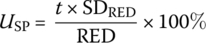
SDRED = standard deviation of the RED values measured for each test condition
t = t‐statistic for a 95% confidence level defined as a function of the number of replicate samples by using the following data (Table 5.17).
- Select the highest USP from all test conditions for calculating the VF.
Table 5.17 t‐Statistic for a 95% confidence level. For reactors using the calculated dose approach, the uncertainty of interpolation (UIN) is calculated as the lower boundary of the 95% prediction interval for the dose‐monitoring equation. This prediction interval reflects the noise in the data about that fit. In nonstatistical terms, the UIN represents the difference between (i) the RED value as derived using measured log inactivation and the UV dose–response curve and (ii) the RED value as calculated using the dose‐monitoring equation. The value of UIN depends on the calculated RED (or calculated dose), increasing at low calculated RED values. EPA recommends that one UIN be selected that represents the most conservative (largest) uncertainty value calculated for the validated dose‐operating range (for the lowest calculated RED). Alternatively, UIN can be expressed as a function of the calculated RED. UIN is calculated using the following equation: where
Table 5.18 t‐Statistic at a 95% confidence level for a sample size equal to the number of test conditions. The last step is to adjust the RED results by the VF to determine the validated dose for the UV reactor using the following equation:
UV intensity set point approach can be used to validate the validated dose through the following example:
Table 5.19 Design specifications. Table 5.20 Characteristics of UV reactor. Table 5.21 Challenge microorganism UV dose–response measured using a collimated beam apparatus. Table 5.22 Flow rate, UVT, lamp power, and UV sensor data measured during validation testing. Table 5.23 Measured influent and effluent challenge microorganism concentrations. Table 5.24 Sensor 1 measurements with lamp 2 operated at 100% ballast power. Table 5.25 Reference UV sensor checks. Figure 5.10 Log N versus UV dose using the data in Table 5.21 at 90% UVT. Figure 5.11 Log I versus UV dose using the data in Table 5.21 at 97% UVT. Table 5.26 Challenge microorganism UV dose–response defined as UV dose versus [log(No/N)] (i.e. log I). Figure 5.12 Log I versus UV dose using the data in Table 5.26.
Number of samples
T
3
3.18
4
2.78
5
2.57
5.3.4.1 Calculating UIN for the Calculated Dose Approach
![]()
Number of data points used to develop the dose‐monitoring equation
T
Number of data points used to develop the dose‐monitoring equation
t
3
3.18
14
2.14
4
2.78
15
2.13
5
2.57
16
2.12
6
2.45
17
2.11
7
2.36
18
2.10
8
2.31
19–20
2.09
9
2.26
21
2.08
10
2.23
22–23
2.07
11
2.20
24–26
2.06
12
2.18
27–29
2.05
13
2.16
≥30
2.04
5.3.4.2 Determining the Validated Dose and Validated Operating Conditions
![]()
Design flow rate
400 gpm
Minimum UVT
90%
Lamp aging factor
80%
Fouling factor
85%
Fouling/aging factor
68% (80% × 85%)
Disinfection goal
2.5‐log Cryptosporidium inactivation credit
UV reactor
UV dose‐monitoring approach
UV intensity set point approach with one alarm set point
90% UVT
97% UVT
UV dose (mJ/cm2)
Replicate 1
Replicate 2
UV dose (mJ/cm2)
Replicate 1
Replicate 2
N (pfu/ml)
Log N
N (pfu/ml)
Log N
N (pfu/ml)
Log N
N (pfu/ml)
Log N
0
882 329
5.95
944 980
5.98
0
1 148 154
6.06
1 300 460
6.11
10
180 120
5.26
198 394
5.30
10
316 328
5.50
257 749
5.41
20
64 217
4.81
69 438
4.84
20
113 644
5.06
74 396
4.87
30
20 622
4.31
20 100
4.30
30
34 679
4.54
25 189
4.40
40
7 257
3.86
8 145
3.91
40
12 624
4.10
9 226
3.97
60
1 274
3.11
1 399
3.15
60
1 980
3.30
1 722
3.24
80
188
2.27
261
2.42
80
387
2.59
211
2.32
100
80
1.90
90
1.95
100
80
1.90
100
2.00
Test ID
Banks on
Flow rate (gpm)
UVT (%)
Relative lamp output (%)
Sduty, 1 (mW/cm2)
Sduty, 2 (mW/cm2)
1
1, 2
394
89.9
100
11.7
11.7
2
1, 2
403
97.0
66
11.6
11.7
Test ID
Influent challenge microorganism log concentration
Effluent challenge microorganism log concentration
Replicate
Replicate
1
2
3
1
2
3
1
5.94
6.00
5.84
4.57
4.54
4.56
2
6.01
5.99
6.04
4.10
4.09
4.06
Lamp ID
Sduty 1 (mW/cm2)
Lamp ID
Sduty 1 (mW/cm2)
1
13.6
5
13.9
2
14.6
6
13.3
3
14.2
7
14.5
4
13.4
8
14.3
Before/after validation testing
UVT(%)
Relative lamp power (%)
Sensor ID
Sduty (mW/cm2)
Sref, 1 (mW/cm2)
Sref, 2 (mW/cm2)
Sref, 3 (mW/cm2)
Before
97
100
1
11.3
11.7
12.1
11.4
Before
97
68
1
5.1
5.5
5.7
5.3
Before
90
100
2
3.7
4.0
4.1
3.8
Before
90
68
2
2.0
1.9
1.9
1.8
After
97
100
1
11.6
11.8
12.2
11.4
After
97
68
1
5.1
5.4
5.6
5.3
After
90
100
2
3.9
4.0
4.1
3.9
After
90
68
2
1.9
1.8
2.0
1.8

90% UVT
97% UVT
UV dose (mJ/cm2)
Replicate 1
UV dose (mJ/cm2)
Replicate 1
Replicate 2
5.92 − log N
Replicate 2
6.05 − log N
0
−0.03
−0.06
0
−0.01
−0.06
10
0.66
0.62
10
0.55
0.64
20
1.11
1.08
20
0.99
1.18
30
1.61
1.62
30
1.51
1.65
40
2.06
2.01
40
1.95
2.08
60
2.81
2.77
60
2.75
2.81
80
3.65
3.5
80
3.46
3.73
100
4.02
3.97
100
4.15
4.05
5.3.5 Collimated Beam Data Uncertainty
The uncertainty in the UV dose calculation using the Equation (5.15):
where
- UDR = uncertainty of the UV dose–response fit at a 95% confidence level
- UV doseCB = UV dose calculated from the UV dose–response curve in Figure 5.12
- SD = standard deviation of the difference between the calculated UV dose–response and the measured values from Table 5.21
- t = t‐statistic at a 95% confidence level for a sample size equal to the number of test condition replicates used to define the dose–response
In this case, SD = 2.2 at 1‐log inactivation and t = 2.04 for 32 test condition replicate as shown in Table 5.26. Equation (5.15) can then be used to determine UDR at various log inactivation values from Table 5.21. The graph in the succeeding text shows the relationship between log inactivation and UDR. The value of UDR should not exceed 30% at the UV dose corresponding to 1‐log inactivation of the challenge organism. In this case, UDR = 25% at 1.0‐log inactivation, which is less than the recommended limit of 30% (Figure 5.13).
Figure 5.13 Uncertainty at different log I levels.
5.3.6 Electrical Energy per Order (EE/O)
The electrical energy (in kilowatt hours) required to reduce the concentration of a pollutant by one order of magnitude for 1000 US gallons of of water is defined as electrical energy per order (EE/O). For batch reactor, the equation is

where
- EEO = electrical energy per order (kWh)
- P = lamp power (kW)
- t = exposure time (min)
- V = reactor volume (l)
- Ci = initial concentration
- Cf = final concentration
For a continuous flow reactor, the equation is
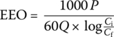
where
- P = lamp power (kW)
- t = exposure time (min)
- Q = flow rate (gpm)
- Ci = initial concentration
- Cf = final concentration
Power requirements can be estimated from manufacturer‐supplied information regarding the number of lamps in a given system, the kilowatt draw of each lamp, the warranty power setting, and the average number of UV reactors needed. The total kilowatt draw from each manufacturer is then determined, and the average power consumption (kW) is calculated. The average power consumption can be used to calculate the total power costs by multiplying the total power requirements by the assumed power rate of 0.076$/kWh. One of the most important concepts to comparing power consumptions for different UV disinfection systems is electrical energy per order (EE/O). Usually, plug flow reactor will require less EE/O than batch reactors because the distribution of UV intensity in the plug flow reactor (PFR) is more uniform than batch reactor. In addition, the equations may not hold at extreme high inactivation orders such as greater than 6 or 7 because most UV dose will be wasted when Giardia concentration is extremely low.
5.4 Exercise
5.4.1 Questions
- Conceptual questions:
- How is reliability of EEIS defined and quantified?
- What are the contributing factors to unit process failure?
- What is ISA?
- What are the advantages for decentralized WRRFs?
- What are the four major spatial scales in assessing reliability of EEIS?
- Please rank the effectiveness of best management practice (BMP) recommended by the United States in the text according to your professional judgment.
- In UV disinfection, what is the RED?
- How would UVT of a water sample affect the UV disinfection efficiency?
- Please rank fluence and cost required by UV disinfection of one cubic meter of drinking water, wastewater effluent, and reclaimed waste water? Why are there different requirements?
- Please rank what are the major factors contributing to the uncertainty in estimating RED?
- Please rank how is the uncertainty of interpolation (UIN) calculated?
- Please rank what are the differences in calculation of the electrical energy per order for batch or CSTR reactors?
- Reliability questions related to WTPs or WTWPs in your own city. In assessing the reliability of local utilities, the US EPA recommended the following questions on reliability level of service:
- What is plant useful life and value?
- What level of service do my stakeholders and customers demand?
- What do the regulators require and what is actual performance?
- How could unit processes of a plant fail and why do they fail?
- What are the likelihoods (probabilities) and consequences of unit process failure?
- What does it cost to repair the unit process and what are the other costs (social, environmental, etc.) that are associated with the failure?
- What alternative strategies exist for managing O&M, personnel, and capital budget to ensure reliability of a plant?
- What are the costs of rehabilitation, repair, and replacement for critical unit processes?
- Do utility companies have enough funding to maintain their plants for the required level of service?
5.4.2 Calculation
- Eisenberg et al. (2001) reported two different criteria in quantifying the reliability of a WWTP. One is the expected time between failure (ETBF) in unit process based on chi‐square distribution. Another is the fraction of the study period that all components in the unit were operating as shown in Table 5.27. Please answer the following:
- Which unit process in the table is the most reliable process in terms of ETBF in days?
- How would the reliability of all the unit processes be ranked?
- In terms of probability of failure, which process is most likely to fail and which one is the least?
- UV doses required to achieve required log inactivation are shown in this chapter. Please develop a Matlab program to do the following using the regression equations presented in this chapter:
- What is the ratio of UV dose required if 4‐, 3‐, and 2‐log inactivation are required for viruses, Giardia, and Crypto?
- What are the strategies you may develop to achieve the three objectives at the lowest cost?
- If a water sample has a UV absorption coefficient at 254 nm of 0.1 and I0 of 120 mJ/cm, please develop a Matlab code to answer the following:
- What would be the UV light intensity reading using a UV absorption photospectroscopy?
- How often would you expect this UVT to occur if the sample was filtered water 2 as described in the example cumulative frequency diagram for three filtered waters by US EPA (2006)?
- According to EPA’s requirement, at least 3‐log inactivation is required for Giardia, if the lamp power is 3 kW. Please answer the following by using Matlab code:
- What would be the EE/O for a batch reactor if the log of inactivation is 3, 4, 5, and 6?
- What would be the EE/O for a flow reactor if the log of inactivation is 3, 4, 5, and 6?
- Please comment on the EE/O values if the log of inactivation is greater than 6.
Table 5.27 Reliability of a WWTP (Eisenberg et al., 2001).
Unit processes
ETBF (days)
Fraction of all components are operating
Headworks
26
0.9953
Primary
41
0.9985
Secondary
9
0.9757
Tertiary
13
0.9994
UV
212
0.9991
Reverse osmosis
10
0.9990
5.4.3 Projects
5.4.3.1 Xiongan Design Project
Xiongan is located in the heart of Hebei province and next to Baiyangdian Lake. The Chinese government is relocating many nongovernmental related businesses and some government entities from Beijing to Xiongan such as science and technology, education, manufacturing, and certain corporations. It could require 350 billion USD in fixed asset investment over the next 20 years. Xiongan district is to expand to 10, 100, and 1000 km2 in 5, 10, and 20 years, respectively. According to this plan, please do the following:
- What is the historical air, water, and solid waste produced in Beijing in the past ten years?
- What would be the required fixed investment and GDP in USD for 5, 10, 15, and 20 years according to the historical data?
- What would be the air, water, and solid wastes in tons for 5, 10, 15, and 20 years if the district is to expand to 10, 100, and 1000 km2 in 5, 10, and 20 years, respectively, according to the historical data?
- How would you incorporate UV disinfection to WWTP and WTP in new Xiongan district? Why?
5.4.3.2 Community Proposal Project
The following topics may be considered:
- After you collected air, water, and wastewater production data on your hometown, you calculated the current air, water, and soil quality indices. You identified that water pollution is the most serious environmental issue in your town. Please develop a proposal to design a sustainable wastewater engineering system for your hometown to achieve water quality indices of 10, 20, and 50% improvement in 5, 10, and 20 years, respectively.
- Can your engineering design be directly applied to your state and your country? If not, what would be different at city, regional, and country levels? How would you improve your design?
- For disinfecting wastewater effluent, the best way is UV. If your community did not use UV disinfection of wastewater effluent, please conduct throughout research on the following:
- Commercially available UV products that are economic for your community to adopt.
- What are the capital costs of the UV equipment?
- What are the validation tests that have to be carried out to satisfy the US EPA UV disinfection credit requirement test to ensure the reliability of the UV system?
- why UV disinfection of treated wastewater is not practiced? Is leachate in wastewater treatment plant a problem preventing UV to be adopted?
- What are the alternatives to co-treatment of leachate with wastewater?
References
- Australia, the Natural Edge Project (TNEP) (2017). Worked example 5‐domestic water systems. http://www.naturaledgeproject.net/Whole_System_Design.aspx (accessed 9 December 2017).
- American Water Works Association and American Society of Civil Engineers (2012). Water Treatment Plant Design, 5e. New York: McGraw‐Hill.
- Chang, J.C.H., Ossoff, S.F., Lobe, D.C. et al.(1985). UV inactivation of pathogenic and indicator micro‐organisms. Applied Environmental Microbiology 49 (6): 1361–1365.
- Draper, N. and Smith, H. (1998). Applied Regression Analysis, 3e. New York: Wiley.
- Eisenberg, D., Soller, J., Sakaji, S., and Olivieri, A. (2001) A methodology to evaluate water and wastewater treatment plant reliability. Water Science & Technology 43 (10): 91–99.
- Sedlak, D. (2014). Water 4.0: The Past, Present, and Future of the World’s Most Vital Resource. New Haven: Yale Press.
- Mackey, E.D., Wright, H.B., Hargy, T. et al.(2006). Optimization of UV Reactor Validation. Denver: American Water Works Association Research Foundation.
- Meng, Q.S. and Gerba, C.P.(1996). Comparative inactivation of enteric adenoviruses, poliovirus and coliphages by ultraviolet irradiation. Water Research 30 (11): 2665–2668.
- Sommer, R., Haider, T., Cabaj, A. et al. (1998a). Time dose reciprocity in UV disinfection of water. Water Science and Technology 38: 145–150.
- Sommer, R., Haider, T., Cabaj, A. et al. (1998b). Time UV dose reciprocity in UV disinfection of water. International Association of Water Quality (IAWQ), Vancouver, 1998 Poster.
- Stasinopoulos, P., Smith, M., Hargroves, K., and Desha, C. (2008) Whole System Design: An Integrated Approach to Sustainable Engineering. Earthscan: The Natural Edge Project.
- USEPA (2006). Ultraviolet disinfection guidance manual for the final long term 2 enhanced surface water treatment rule, 2006. http://www.epa.gov/safewater/disinfection/lt2/pdfs/guide_lt2_uvguidance.pdf (accessed 13 December 2017).
- Wilson, B.R., Roessler, P.F., van Dellen, E. et al.(1992). Coliphage MS2 as a UV water disinfection efficacy test surrogate for bacterial and viral pathogens. Proceedings of the American Water Works Association Water Quality Technology Conference, Toronto, Canada (November 15–19).
- Wright, H.B. (2006). Carollo Engineers. Internal communication with Erin Mackey, Carollo Engineers.