8
Efficiency of Renewable Energy
The solar energy harnessed and used measures human civilization.
8.1 Principle 5
The efficiency of renewable energy such as biomass, solar, and wind should be maximized for all the EEIS. In gauging a civilization, mankind is at its infancy because only 0.75% of solar energy is currently harnessed for human activities. If the efficiency of solar cell were to double, the amount of renewable energy harvested could increase significantly. For example, if 2% of solar energy that reached the Earth could be efficiently utilized, human civilization could reach to the next level. If 2% of energy in the Milky Way galaxy reached the Earth and were harnessed by humans, mankind could colonize most nearby planets. However, it is estimated that about 100 years is needed to harvest 2% of the solar power.
To reduce operation cost of WWTP, the best way is to generate renewable energy such as electricity and heat while increasing energy efficiency of the WWTP. Therefore, energy efficiency is a critical step to retrofit WWTP to energy positive or design and build new WRRF.
Table 8.1 SEE design metrics.
| Design | Problems | Energy |
| Air | Incomplete combustion | Efficiency of any conversion process is less than 100% |
| Water | AS in WWTP | Energy intensive and not productive |
| Land | Pollutants in runoff | Regenerative design for biomass production |
| Ecological | Energy efficiency in food chain | Higher energy efficiency process |
Before major improvements of EEIS energy efficiency were started across the United States in 2008, design standards of WWTP and WTP have not changed for the last 100 years since the introduction of the activated sludge process in 1916. Major design theory in air, water, and solid waste management was taught without data and tools critical to design sustainable EEIS. The traditional design philosophy of one size fits all resulted in urgent environmental issues and challenges. For example, to calculate the loading factors, chemical oxygen demand (COD) is used to quantify organic matter in terms of oxygen, while the concept of biological oxygen demand (BOD) was specifically designed for biological treatment of wastewater using activated sludge. As a result, COD and BOD intrinsically represent pollutants in terms of oxygen needed to oxidize and are not meant to represent how much energy is embedded in the organic compounds. Only recently was the intrinsic energy contained in the organic pollutants considered as energy resource to be recovered in the design. The paradigm is shifting from organic pollutants as an energy liability required by aeration to energy source to be recovered. In theory, 1.7 kWh energy is contained in one cubic meter of a typical domestic wastewater in the United States. If only 25% of the energy were to be recovered, it could reach energy neutral to run the WWTP at 0.3 kWh/m3. However, no design criteria in terms of energy efficiency were established to ensure the sustainability of the EEIS. No ranking system exists to assess the sustainability of WWTP or recovery of materials. For these reasons, many challenging questions beg answers: How did the EEIS in the past get it so wrong in designing energy negative WWTPs? How can we treat our wastewater better in terms of minimal footprint on water, energy, and nutrients? What are the regenerative ways to design WWTP? Conceptual, technology, cost, and professional isolation may all contribute to the current challenges faced by the United States and all over the world. Fundamental sciences of thermodynamics may offer us a starting point to shine light into this paradigm shift through creative thinking.
8.2 Challenges and Opportunities
Solar energy has a unit radiation intensity of 1366 W/m2 and is clean, free, abundant, and reliable renewable energy. If all the solar energy were captured and stored, it could provide all the energy in one day consumed by the mankind for 1 year. Due to low efficiency of energy conversion, however, only 0.1% of 100 000 terawatts (TW) were captured by biomass through photosynthesis. These 100 TW biomasses would be consumed by herbivores to store 10 TW, primary carnivores to store 1 TW, and secondary carnivores to store 0.1 TW. Considering that the total human demand is 15 TW, 15% of primary biomass would meet human demand. Therefore, biomass is a natural candidate to harvest the solar energy in nature. For this reason, algae farming through wastewater is an important emerging technology for future renewable energy. In addition, radiant heat and light from the sun could be harnessed through photovoltaics, solar heating, artificial photosynthesis, solar architecture, and solar thermal electricity.
To achieve zero energy design, solar energy will play critical role to provide electricity or hot water as unit cost of solar photovoltaic technology decreases. To appreciate solar energy, it is important to point out that it is also the sun that produced the fossil fuels such as coal, oil, and natural gas in billion years of Earth’s evolution. The National Academy of Engineering proposed the following grand plan for replacing fossil fuel with renewable energy as shown in Figure 8.1. First, in the next 20 years (2005–2025) of continued use of fossil fuels (especially oil) as the predominant source of energy and chemical feedstocks, managing carbon, reducing the intense use of energy resources, and promoting sustainability through educational efforts will be critical. Second, in the next 20–100 years (2025–2105), the use of fossil fuels will be phased out, and the ability to carry out green chemistry and engineering (built on fundamental understanding of the full life cycle impacts and toxicology of chemicals) and having access to alternative renewable sources of fuels and feedstocks will then be critical. In designing EEISs, SEE needs to synchronize the pace of the paradigm shift and contribute to this grand vision. For example, by 2025 all the WWTPs in the United States should be retrofitted to energy positive as energy‐production centers, recovery of nutrients by 2035, and recover all the materials by 2045.
Figure 8.1 The grand challenges (box) for sustainability (arrow) address the transition from current thinking to the ideal vision for the chemical industry over the next 100 years.
(Source: Reprint with permission from the National Academy of Science.)
In the past, EE designers failed to harvest large potential energy and resource from wastewater because they were encouraged to optimize only parts of the system such as pumps in WWTPs. Components are optimized in isolation from other components; optimization typically considers single rather than multiple benefits. The optimal sequence of design steps is not usually considered because the designers have become highly specialized in their own professions. Integrated engineering design (IED) optimization has not been fully utilized to optimize the whole system. However, IED could enable designers to achieve efficiency improvements from 75 to 95% and to reduce environmental impacts due to the increased efficiency.
8.2.1 Inefficient Combustion of Fossil Fuels
The combustion of fossil fuels results in pollutant emissions that can damage human health and the environment on a number of levels. Most environmental concern has recently focused on global warming induced by the emission of so‐called “greenhouse” gases (GHGs), principally CO2 emissions from fossil fuel combustion. However, combustion has very low efficiency. Table 8.2 lists the energy efficiency of a coal‐powered electrical station. To design the most energy‐efficient EEIS, the overall energy efficiency can be estimated using an IED approach. For example, an electric motor driving a pump that transports wastewater in WWTP comprises:
- An electric motor (sizing and efficiency rating)
- Motor controls (switching, speed or torque control)
- Motor drive system (belts, gearboxes, etc.)
- Pump
- Pipework
- Demand for fluid.
Table 8.2 Thermodynamic performance of coal‐fired power stations. Source: Stasinopoulos et al. (2008). a Efficiencies based on gross calorific or higher heating value (HHV) of fuels.
Plant components
Energy losses (% of plant input)
Exergy losses (% of plant input)
Steam generator
9.0
49.0
Combustiona
(29.7)
Heat exchangera
(14.9)
Thermal stack lossa
(0.6)
Diffusional stack lossa
(3.8)
Turbines
0
4.0
Condenser
47.0
1.5
Heaters
0
1.0
Miscellaneous
3.0
5.5
Plant totals
59.0
61.0
Generation efficiencies
Z = 100 − 59 = 41
η = 100 − 61 = 39
The efficiencies of these elements interact in complex ways. For example, if each element in the chain is improved in efficiency by 10%, then the overall level of energy use is ![]() , which results in a saving of 47%. Therefore, an IED approach could yield over 50% improvements. Corresponding to the energy efficiency improvement is the correlated reductions in negative environmental impacts. If the most efficient component is chosen for each part of a motor system, overall the efficiency of the whole system would be about seven times greater as shown in Table 8.3.
, which results in a saving of 47%. Therefore, an IED approach could yield over 50% improvements. Corresponding to the energy efficiency improvement is the correlated reductions in negative environmental impacts. If the most efficient component is chosen for each part of a motor system, overall the efficiency of the whole system would be about seven times greater as shown in Table 8.3.
Table 8.3 Comparison of the best versus worst efficiency motoring systems (Stasinopoulos et al., 2008).
| System component | Best efficiency | Worst efficiency |
| Electrical wiring | 0.98 | 0.9 |
| Motor | 0.92 | 0.75 |
| Drive (e.g. gearbox or belt) | 1.0 | 0.7 |
| Pump | 0.85 | 0.4 |
| Pipes | 0.9 | 0.5 |
| Overall efficiency of system | 0.69 | 0.095 |
8.2.2 Challenges in China
In China, intensive fossil fuel consumption causes severe smog, which results in damage to human health and the environment. As a result, the Chinese government (2017) plans to reduce energy consumption as shown in Tables 8.4, 8.5, 8.6, 8.7, 8.8, and 8.9.
Table 8.4 China energy consumption reduction target in the 13th FYP.
| Regions | Energy reduction target in the 13th FYP (%) | Total energy consumption in 2015 (million tons of standard coal) | Energy consumption reduction target in the 13th FYP (million tons of standard coal) |
| Beijing | 17 | 6 853 | 800 |
| Tianjin | 17 | 8 260 | 1040 |
| Hebei | 17 | 29 395 | 3390 |
| Shanxi | 15 | 19 384 | 3010 |
| Inner Mongolia | 14 | 18 927 | 3570 |
| Liaoning | 15 | 21 667 | 3550 |
| Jilin | 15 | 8 142 | 1360 |
| Heilongjiang | 15 | 12 126 | 1880 |
| Shanghai | 17 | 11 387 | 970 |
| Jiangsu | 17 | 30 235 | 3480 |
| Zhejiang | 17 | 19 610 | 2380 |
| Anhui | 16 | 12 332 | 1870 |
| Fujian | 16 | 12 180 | 2320 |
| Jiangxi | 16 | 8 440 | 1510 |
| Shandong | 17 | 37 945 | 4070 |
| Henan | 16 | 23 161 | 3540 |
| Hubei | 16 | 16 404 | 2500 |
| Hunan | 16 | 15 469 | 2380 |
| Guangdong | 17 | 30 145 | 3650 |
| Guangxi | 14 | 9 761 | 1840 |
| Hainan | 10 | 1 938 | 660 |
| Chongqing | 16 | 8 934 | 1660 |
| Sichuan | 16 | 19 888 | 3020 |
| Guizhou | 14 | 9 948 | 1850 |
| Yunnan | 14 | 10 357 | 1940 |
| Tibet | 10 | — | — |
| Shaanxi | 15 | 11 716 | 2170 |
| Gansu | 14 | 7 523 | 1430 |
| Qinghai | 10 | 4 134 | 1120 |
| Ningxia | 14 | 5 405 | 1500 |
| Xinjiang | 10 | 15 651 | 3540 |
Table 8.5 China emission reduction target of chemical oxygen demand (COD) in the 13th FYP.
| Regions | Emission in 2015 (million tons) | Emission reductions in 2020 (%) | Emission reduction of key projects in 2020 (million tons) |
| Beijing | 16.2 | 14.4 | 2.33 |
| Tianjin | 20.9 | 14.4 | 2.47 |
| Hebei | 120.8 | 19 | 16.14 |
| Shanxi | 40.5 | 17.6 | 4.75 |
| Inner Mongolia | 83.6 | 7.1 | 5.19 |
| Liaoning | 116.7 | 13.4 | 8.41 |
| Jilin | 72.4 | 4.8 | 2.32 |
| Heilongjiang | 139.3 | 6 | 7.33 |
| Shanghai | 19.9 | 14.5 | 2.72 |
| Jiangsu | 105.5 | 13.5 | 10.39 |
| Zhejiang | 68.3 | 19.2 | 7.64 |
| Anhui | 87.1 | 9.9 | 7.7 |
| Fujian | 60.9 | 4.1 | 2.14 |
| Jiangxi | 71.6 | 4.3 | 2.73 |
| Shandong | 175.8 | 11.7 | 13.3 |
| Henan | 128.7 | 18.4 | 16.98 |
| Hubei | 98.6 | 9.9 | 8.25 |
| Hunan | 120.8 | 10.1 | 10.49 |
| Guangdong | 160.7 | 10.4 | 11.06 |
| Guangxi | 71.1 | 1 | 0.35 |
| Hainan | 18.8 | 1.2 | 0.16 |
| Chongqing | 38 | 7.4 | 2.36 |
| Sichuan | 118.6 | 12.8 | 14.09 |
| Guizhou | 31.8 | 8.5 | 2.77 |
| Yunnan | 51 | 14.1 | 5.85 |
| Tibet | 2.9 | — | — |
| Shaanxi | 48.9 | 10 | 2.63 |
| Gansu | 36.6 | 8.2 | 2.4 |
| Qinghai | 10.4 | 1.1 | 0.07 |
| Ningxia | 21.1 | 1.2 | 0.1 |
| Xinjiang | 56 | 1.6 | 0.71 |
| Xinjiang production and construction corps | 10 | 1.6 | 0.04 |
Table 8.6 China emission reduction target of ammonia nitrogen in the 13th FYP.
| Regions | Emission in 2015 (million tons) | Emission reductions in 2020 (%) | Emission reduction of key projects in 2020 (million tons) |
| Beijing | 1.6 | 16.1 | 0.24 |
| Tianjin | 2.4 | 16.1 | 0.38 |
| Hebei | 9.7 | 20 | 1.59 |
| Shanxi | 5 | 18 | 0.61 |
| Inner Mongolia | 4.7 | 7 | 0.28 |
| Liaoning | 9.6 | 8.8 | 0.85 |
| Jilin | 5.1 | 6.4 | 0.2 |
| Heilongjiang | 8.1 | 7 | 0.48 |
| Shanghai | 4.3 | 13.4 | 0.53 |
| Jiangsu | 13.8 | 13.4 | 1.25 |
| Zhejiang | 9.8 | 17.6 | 0.85 |
| Anhui | 9.7 | 14.3 | 1.07 |
| Fujian | 8.5 | 3.5 | 0.3 |
| Jiangxi | 8.5 | 3.8 | 0.32 |
| Shandong | 15.3 | 13.4 | 1.49 |
| Henan | 13.4 | 16.6 | 1.93 |
| Hubei | 11.4 | 10.2 | 1.02 |
| Hunan | 15.1 | 10.1 | 1.41 |
| Guangdong | 20 | 11.3 | 1.54 |
| Guangxi | 7.7 | 1 | 0.08 |
| Hainan | 2.1 | 1.9 | 0.04 |
| Chongqing | 5 | 6.3 | 0.32 |
| Sichuan | 13.1 | 13.9 | 1.74 |
| Guizhou | 3.6 | 11.2 | 0.41 |
| Yunnan | 5.5 | 12.9 | 0.67 |
| Tibet | 0.3 | — | — |
| Shaanxi | 5.6 | 10 | 0.38 |
| Gansu | 3.7 | 8 | 0.28 |
| Qinghai | 1 | 1.4 | 0.01 |
| Ningxia | 1.6 | 0.7 | 0.01 |
| Xinjiang | 4 | 2.8 | 0.09 |
| Xinjiang production and construction corps | 0.5 | 2.8 |
Table 8.7 China emission reduction target of SO2 in the 13th FYP.
| Regions | Emission in 2015 (million tons) | Emission reductions in 2020 (%) | Emission reduction of key projects in 2020 (million tons) |
| Beijing | 7.1 | 35 | 1.8 |
| Tianjin | 18.6 | 25 | 2.8 |
| Hebei | 110.8 | 28 | 18.4 |
| Shanxi | 112.1 | 20 | 22.4 |
| Inner Mongolia | 123.1 | 11 | 13.5 |
| Liaoning | 96.9 | 20 | 14.4 |
| Jilin | 36.3 | 18 | 5.2 |
| Heilongjiang | 45.6 | 11 | 4.3 |
| Shanghai | 17.1 | 20 | 3.4 |
| Jiangsu | 83.5 | 20 | 13.3 |
| Zhejiang | 53.8 | 17 | 9.1 |
| Anhui | 48 | 16 | 5.2 |
| Fujian | 33.8 | — | 3.5 |
| Jiangxi | 52.8 | 12 | 6.3 |
| Shandong | 152.6 | 27 | 35 |
| Henan | 114.4 | 28 | 20.5 |
| Hubei | 55.1 | 20 | 10.9 |
| Hunan | 59.6 | 21 | 8.5 |
| Guangdong | 67.8 | 3 | 2 |
| Guangxi | 42.1 | 13 | 4.5 |
| Hainan | 3.2 | — | 0.4 |
| Chongqing | 49.6 | 18 | 8.1 |
| Sichuan | 71.8 | 16 | 11.2 |
| Guizhou | 85.3 | 7 | 6 |
| Yunnan | 58.4 | 1 | 0.6 |
| Tibet | 0.5 | — | — |
| Shaanxi | 73.5 | 15 | 11 |
| Gansu | 57.1 | 8 | 4.6 |
| Qinghai | 15.1 | 6 | 0.9 |
| Ningxia | 35.8 | 12 | 4.3 |
| Xinjiang | 66.8 | 3 | 2 |
| Xinjiang production and construction corps | 11 | 13 | 0.9 |
Table 8.8 China emission reduction target of nitrogen oxides in the 13th FYP.
| Regions | Emission in 2015 (million ton) | Emission reductions in 2020 (%) | Emission reduction of key projects in 2020 (million tons) |
| Beijing | 13.8 | 25 | 0.7 |
| Tianjin | 24.7 | 25 | 3.5 |
| Hebei | 135.1 | 28 | 19.9 |
| Shanxi | 93.1 | 20 | 16.3 |
| Inner Mongolia | 113.9 | 11 | 12.5 |
| Liaoning | 82.8 | 20 | 14.9 |
| Jilin | 50.2 | 18 | 9 |
| Heilongjiang | 64.5 | 11 | 7.1 |
| Shanghai | 30.1 | 20 | 5.2 |
| Jiangsu | 106.8 | 20 | 18.7 |
| Zhejiang | 60.7 | 17 | 10.3 |
| Anhui | 72.1 | 16 | 9 |
| Fujian | 37.9 | — | 4.6 |
| Jiangxi | 49.3 | 12 | 5.9 |
| Shandong | 142.4 | 27 | 31 |
| Henan | 126.2 | 28 | 15.8 |
| Hubei | 51.5 | 20 | 5.9 |
| Hunan | 49.7 | 15 | 6.3 |
| Guangdong | 99.7 | 3 | 3 |
| Guangxi | 37.3 | 13 | 3.3 |
| Hainan | 9 | — | 1.2 |
| Chongqing | 32.1 | 18 | 2.8 |
| Sichuan | 53.4 | 16 | 3.7 |
| Guizhou | 41.9 | 7 | 2.9 |
| Yunnan | 44.9 | 1 | 0.4 |
| Tibet | 5.3 | — | — |
| Shaanxi | 62.7 | 15 | 9.4 |
| Gansu | 38.7 | 8 | 3.1 |
| Qinghai | 11.8 | 6 | 0.7 |
| Ningxia | 36.8 | 12 | 4.4 |
| Xinjiang | 63.7 | 3 | 1.9 |
| Xinjiang production and construction corps | 9.9 | 13 | 1.3 |
Table 8.9 China emission reduction target of volatile organic carbon in the 13th FYP.
| Regions | Emission in 2015 (million tons) | Emission reductions in 2020 (%) | Emission reduction of key projects in 2020 (million tons) |
| Beijing | 23.4 | 25 | 3.5 |
| Tianjin | 33.9 | 20 | 4.6 |
| Hebei | 154.6 | 20 | 19.5 |
| Liaoning | 105.4 | 10 | 10.5 |
| Shanghai | 42.1 | 20 | 8.4 |
| Jiangsu | 187 | 20 | 31.2 |
| Zhejiang | 139.2 | 20 | 25.5 |
| Anhui | 95.9 | 10 | 9.2 |
| Shandong | 192.1 | 20 | 38.4 |
| Henan | 167.5 | 10 | 16.6 |
| Hubei | 98.7 | 10 | 9.9 |
| Hunan | 98.3 | 10 | 7.9 |
| Guangdong | 137.8 | 18 | 20.7 |
| Chongqing | 40.2 | 10 | 4 |
| Sichuan | 111.3 | 5 | 5.6 |
| Shaanxi | 67.5 | 5 | 3.4 |
8.3 Energy Conservation Laws
Sustainable design alternatives are constrained by basic physical laws and costs. We start with the thermodynamic laws, then exergy, and lastly, technical benchmark data of different processes of WWTPs.
8.3.1 Thermodynamics Laws
Thermodynamic constraints and principles are applicable across both ecological and economic systems. Economic activity is entropic, while entropy increases as order decreases. Entropy leads the tendency of matter and energy to degrade or disperse into less useful forms during economic activity, although waste could be converted back to resources. Recycling of materials could close the loop of materials within society. The second law of thermodynamics requires that materials used in the economy tend to be used entropically. They get dissipated within the economic system unless reused or recovered. However, energy resource is usually degraded and difficult to be recycled depending upon the energy degradation rate. Typically, low‐entropy matter/energy comes in, while high‐entropy matter/energy goes out. The irreversibility of the real processes implies exergy destruction and waste discharged to the environment. Ecological economics starts from a recognition of the environmental, technological, individual, and social sources and support systems of productivity. Both natural and economic capitals should be maximally utilized. Table 8.10 is a brief history of sustainability by applying thermodynamic laws.
Table 8.10 Brief history of applying thermodynamic laws to sustainability limit of economic activities.
| Year | Author | Research work | References |
| 1969 | R. U. Ayres and A. V. Kneese | Introduced mass and energy balances into static input–output analysis | Ayres and Kneese (1969) |
| 1971 | N. Georgescu‐Roegen | Consequences of thermodynamic laws for economic analysis | Georgescu‐Roegen (1971) |
| 1986 | Perrings | Extended input–output analysis to linear dynamic models that showed instabilities of economic activity | Perrings (1986) |
| 1992 | Van Gool W. | Exergy analysis of industrial processes | Van Gool (1992) |
| 2006 | F. C. Krysiak | Mass and energy conservation with the second law of thermodynamics may challenge the fundamental concepts of economic analysis | Krysiak (2006) |
| 2009 | Geoffrey P. Hammond and Adrian B. Winnett | Thermodynamic ideas on ecological economics | Hammond and Winnett (2009) |
8.3.2 The First Thermodynamic Law
The first thermodynamic law defines conservation of materials and energy, which are not to be created or destroyed. Pearce and Turner (1990) analyzed the production process waste in the environment–economy interaction. The processing of resources creates waste WR, as with overburden tips at coal mines; production creates waste WP in the form of industrial effluent and air pollution and solid waste; final consumers create waste WC by generating sewage and municipal solid wastes. The amount of waste in any period equals the amount of natural resources used, R:
The first law of thermodynamics states that energy and matter cannot be created or destroyed, but only transformed. Due to insatiable human demand, mining depletes natural resource, while consumers discard waste into the environment. As a result, mounting tasks are in front of the new generation of SEE designers to sustainably manage air, water, and solid wastes produced by modern societies.
8.3.3 The Second Thermodynamic Law
The second thermodynamic law states that work input into a system can be fully converted to heat and internal energy (via dissipative processes) without perfect efficiency. The maximum amount of work achievable in a given system with different energy sources in reference to its surrounding is referred as exergy. Exergy is the available energy for conversion from a donating source (or reservoir) with reference to a specified datum under ambient environmental conditions. It predicts the theoretical maximum energy available. Usually, high exergy degrades to low exergy continuously and irrevocably.
8.3.3.1 Energy Conversion
8.3.3.2 Enthalpy
Enthalpy is the heat content of gases, which depends not only on the internal energy (U) but also on the pressure (P) and volume (V). Thermodynamically, enthalpy is defined as
where
- H = enthalpy (kJ)
- U = internal energy (kJ)
- P = pressure (kPa)
- V = volume (m3)
The reaction heat is the enthalpy change of a reaction:
If there is no pressure change, then this is the heat absorbed:
8.3.3.3 Conservation of Energy
For nonbiodegradable materials in wastewater such as cellular fiber from papers, incineration could be the best process to recover heat energy (Figure 8.2). However, for a thermal power plant, about one‐fourth or one‐third of exergy is wasted due to the inefficiency of mixing and heat loss. On the other hand, chemical efficiency is usually much higher at 94–97%. For this reason, a fuel cell is a much more efficient electricity generation process than a thermal power plant.

Figure 8.2 An energy balance for a simple control volume or unit operation.
8.4 Energy Balances
Energy balances are analogous to mass balances because energy can be neither created nor destroyed. A system can be defined by the boundary separating the system from its surroundings. Open systems refer to mass and energy transfer across system boundaries, while a closed system is only energy transfer across system boundaries. Internal energy (U) is associated with mass by virtue of its state (phase) and temperature. Enthalpy (H) is associated with mass by virtue of its state, temperature, and pressure:
where
- H = enthalpy (kJ)
- U = internal energy (kJ)
- P = pressure (kPa)
- V = volume (m3)
Energy changes in a system are a function of mass and energy inputs and outputs. For systems involving only solids and liquids, the PV term is essentially constant, so ΔU = ΔH:
where
- M = mass
- CV = specific heat (J/kg/°C, BTU/lb/°F, cal/g /°C)
- ΔT = change in temperature
When a substance changes phases, there are changes in internal energy and enthalpy not directly related to temperature change. Energy required from solid to liquid is referred as the enthalpy of fusion, while energy required from liquid to gas is called the enthalpy of vaporization.
Energy can be transferred through conduction, convection, and radiation. Conduction normally associated with solids, e.g., vibrational energy of hotter molecules translated to adjacent molecules:
where
- q = heat transfer rate (J/s)
- htc = thermal conductivity (J/s/m/K)
- A = cross‐sectional area (m2)
- T = temperature (K)
- ΔT = change in temperature (K)
- x = linear distance corresponding to temperature differential (m)
Convection transfers heat from a fluid as a result of movement of the fluid and contact with another substance. For example, a pump or blower causes coolant in auto or hot air from a heat duct by forced convection, while natural convection is a result of density differences and plays an important role in designing energy positive residential houses.
Empirical equation for convective heat transfer between a fluid and surface can be expressed as
where
- hc = system‐specific constant (J/s/m2/K)
- Tf = temperature of the fluid
- Ts = temperature of the surface
In the second law of thermodynamics, there is always inefficiency when energy is converted to work because waste heat is always produced.
8.4.1 Physical Framework by Thermodynamics
Energy, entropy, and exergy have been applied in environmental sustainability. Energy transformations within society have been viewed as resource depletion and environmental degradation by ecology, economics, and engineering.
Figure 8.3 shows that there is a trade‐off between capital cost, which is referred to as embodied energy, and OM cost.

Figure 8.3 Trade‐off between capital and operating costs.
(Source: Adapted from Hammond and Winnett (2009).)
Figure 8.4 plots the energy consumption against equipment size. There is a minimal value associated with the total energy requirement at a specific equipment size, which is also referred to as capital cost.
Figure 8.4 Trade‐off between product energy and equipment size.
(Source: Adapted from Hammond and Winnett (2009).)
Hammond and Winnett (2009) argued that although the thermodynamic (or exergetic) improvement potential is around 80%, only about 50% of energy currently used could be saved by technical means, and when economic barriers are taken into account, this is reduced to perhaps some 30%. Nevertheless, there is significant potential for improvement in energy efficiency as shown in Figure 8.5.
Figure 8.5 The energy efficiency gap between theory and practice.
(Source: Adapted from Hammond and Winnett (2009).)
8.4.2 Exergy
Exergy is the maximum theoretical work that a system can do before being brought into equilibrium with its environment. It is not conserved due to irreversibility, friction, or heat loss due to temperature difference. Exergy represents a theoretical thermodynamic value, while energy efficiency reflects an actual system. It measures the thermodynamic efficiency of a system by reflecting the quality of an energy carrier. In other words, exergy is simply a measure of the maximum theoretical useful work that is obtainable from a thermal system (as it is brought into equilibrium with its surrounding environment). Therefore, exergy analysis should be employed as a tool among several quantitative approaches to study energy systems, in addition to the traditional first law energy analysis:
where
- E = exergy
- U = internal energy
- P = pressure
- V = volume
- T = thermodynamic temperature
- S = entropy
- ΔKE = change in kinetic energy
- ΔPE = change in potential energy
- Subscript “o” = reference environmental state
When a system is not moving nor has potential energy, it can be simplified as
Material resources are viewed as having chemical exergy, because of their disequilibrium with surrounding conditions. An increase in process efficiency will reduce the amount of waste and exergy degradation. Thus, exergy is seen as a measure of the value of the material, whereas process wastes have a potential to cause adverse changes in the environment. The exergy can be used as a potential tool for resource and/or emission accounting.
8.5 Benchmarks for Unit Energy Consumption in WTP and WWTP
8.5.1 Unit Energy Consumption Values in WTP
For energy auditing in water treatment plants, typical unit value of energy consumption for each unit process of a WTP is very important. Table 8.11 compiles these unit values for WTP from Howe et al. (2012). It could be used as a benchmark in conducting energy auditing of any WTP.
Table 8.11 Unit energy consumption and retrofitting measures for water treatment plants.
Source: Data from Howe et al. (2012).
| Unit process | Operation condition | Unit energy consumption (kWh/m3) | Retrofitting measures |
| Coagulation | G = 1200 (1/s) | 0.0004 (theoretical) | Motionless mixer |
| t = 1 (s) | 0.0014 (in practice) | ||
| Flocculation | G = 50 (1/s) | 0.0013 | Motionless mixer |
| t = 30 (min) | |||
| Sedimentation | Δh = 0.6 m (2 ft) | 0.0016 | Plate or tube settler |
| Granular filtration | Δh = 5–4 m during filtration | 0.01–0.014 | Increasing filtration rate from 10 to 15 m/h (4–6 gpm/ft2), total filter area decreases 33% |
| Δh = 1 m (4 gpm/ft2) every 24 h interval for backwashing | 0.0007–0.0031 | Reduce solid concentration before filtration | |
| Membrane filtration | Low flux 6 gal/ft2/day (or 10 l/m2/h) | 0.022 | Impacts: global warming, human, aquatic, marine, and terrestrial toxicity |
| Multistage stage membrane filtration | |||
| Medium flux 18–36 gal/ft2/day (or 30–60 l/m2/h) | Photooxidant formation potential | Multistage stage membrane filtration | |
| Eutrophication | Dead‐end flow is better than cross‐flow membrane filtration | ||
| Reverse osmosis | TDS 35 000 mg/l | 5.6 | Better membrane |
| 50% recovery | Two or more stages with booster pumps between stages | ||
| 85 bar (1230 psi) | Water recovery rate varies from 50 to 85% | ||
| Brine concentrators and crystallizers | |||
| Adsorption | ΔP = 1.7 bar (25) | 0.06 | Regeneration of 1 kg GAC releases 2–5 kg CO2 |
| Ion exchange | ΔP = 1.7 bar (25) | 0.06 | Brine management by evaporation ponds and falling film evaporator |
| Air stripping | Countercurrent packed towers with height from 10 to 15 m | From 0.051 to pump water to 15 m | Optimal air/water = 3.5 for minimal pressure drop from 50 to 100% |
| 0.025–0.051 for air blower | |||
| Advanced oxidation process | O3: 6–10 kWh/kg O3 | 0.04–0.08 | Fine bubble diffuser to increase mass transfer of O3 |
| 4–6 mg/l | |||
| H2O2: 2–4 kWh/kg H2O2 | 0.003–0.01 | Optimal pH | |
| H2O2/O3 | 0.043–0.09 | Optimal pH and fine bubble diffuser to increase mass transfer of O3 | |
| H2O2 1.4–2.8 mg/l | |||
| UV | |||
| 40 mJ/cm2 for disinfection | 0.003–0.025 | Reduce turbidity of water | |
| 100–1000 mJ/cm2 for oxidation | 0.0075–0.63 | Better UV reactor design | |
| UV/H2O2 | |||
| H2O2 3–5 mg/l | 0.01–0.9 | Optimal pH | |
| H2O2 3–100 mg/l for remediation | 0.004–0.28 | Better UV reactor design |
8.5.2 Unit Energy Consumption Values in WWTP
For WWTPs, unit energy consumption data are extremely important when energy auditing is carried out in a WWTP. More importantly, the benchmark data for each unit process are critical to identify the energy gaps where energy efficiency could be improved by retrofitting the current WWTPs. Table 8.12 lists unit energy consumption data of each unit process of WWTP.
Table 8.12 Unit values of benchmark parameters.
| Benchmark parameters | Unit values |
| Energetic content of methane | 803 kJ/mol |
| Energetic content of hydrogen gas | 286 kJ/mol |
| Biomass caloric content | 20.4–25.6 MJ/kg fuel |
| Biomass heat content by combustion with 0.7 efficiency | 14.2–21.4 MJ/kg fuel |
| Crude oil heat content by hydrothermal | 33.2 MJ/kg fuel |
| Liquefaction with efficiency from | |
| Methane by anaerobic digestion with efficiency from 0.4 to 0.6 | 35.8 MJ/kg fuel |
| Biodiesel by transesterification with efficiency from 0.1 to 0.3 | 37.2 MJ/kg fuel |
| N/P limited determination (Redfield ratio) | <16 is N limited |
| Energy content of COD | 3.86 kWh/kg COD |
| Combustion energy yield | 14.2–21.4 MJ/kg |
| COD production·per capita per day | 180 |
| N production per capita per day | 13 |
| P production per capita per day | 2.1 |
| Lipid storage compound | Stearic acid (C18H36O2) |
| Carbohydrate storage compound | Glucose (C6H12O6) |
| Protein compound | C16H24O5N4 |
In the net zero guideline for WWTP, best practice values are significantly less than the typical value among 24 WWTPs surveyed in New York (Trarallo et al., 2015), so there is great potential to improve the performance of energy inefficient processes so that WWTPs can be retrofitted to be energy positive. In the last decade, major research efforts have been carried out all over the world such as in Singapore and Beijing, China (Gans et al., 2007) (Table 8.13). It shows that the overall energy efficiencies of WWTPs in Jurong and Gaobeidian are 35.9 and 31%, respectively. Since aeration and dewatering are the most energy‐intensive processes, typical and best practice values in terms of per kg pollutant removed, and unit energy consumptions in WWTPs all over the world have been compared in Table 8.14.
Table 8.13 Comparison of overall plant‐specific energy consumption between Jurong (Singapore) and Gaobeidian, Beijing (China) (Gans et al., 2007).
| Jurong | Gaobeidian, Beijing | |
| Population served (PE) | 0.99 million | 2.4 million |
| Flow (m3/day) | 0.154 million | 1 million |
| BOD5 (mg/l) | 329 | 173 |
| COD (mg/l) | 924 | 346 |
| Total electricity consumption (kWh/m3) | 0.45 | 0.258 |
| Total electricity consumption (kWh/kgCOD) | 0.58 | 0.746 |
| Total electricity consumption (kWh/kgO2D) | 0.58 | 0.443 |
| Preliminary (kWh/m3) | 0.002 | 0.083 |
| Fine screen‐perforated plate, horizontal flow grit chamber | Coarse screen (6), fine screen (4), and grit chamber | |
| Primary treatment (kWh/m3) | 0.0012 | 0.015 |
| Gravity sedimentation | Traveling bridge, mixer, shredder, sludge pump | |
| Aeration (kWh/m3) | 0.169 | 0.1484 |
| Surface‐fixed and variable speed aerators | Centrifugal blowers, fine bubble aerators, mixer | |
| Sludge thickening (kWh/m3) | 0.003 | 0.002 |
| Dissolved air flotation | Gravity thickening | |
| Sludge dewatering (kWh/m3) | 0.021 | 0.003 |
| Centrifuge, belt filter press | Belt filter press | |
| Digester (kWh/m3) | 0.043 | 0.007 |
| Draft tube system, gas injection system, mesophilic, no external heating | Mesophilic, external heating: spiral‐plate heat exchange | |
| Pump system (kWh/m3) | 0.151 | — |
| Total electricity generation(kWh/m3) | 0.160 | 0.081 |
| Gas collection, genset electricity generation | Gas holder for collected gas, methane booster compressor (8) | |
| Energy efficiency (%) | 35.9 | 31 |
Table 8.14 Unit energy consumption of WWTP at various locations.
| Energy consumption (kWh/m3) | Austria | Austria (Strass) | Sweden | China (Beijing) | Japan | Iran |
| Total energy consumption | 0.304 | 0.317 | 0.475 | 0.258 | 0.320 | 0.300 |
| Preliminary | 0.039 | 0.068 | 0.136 | 0.083 | 0.013 | 0.013 |
| Primary | — | 0.015 | 0.001 | |||
| Aeration | 0.212 | 0.181 | 0.226 | 0.148 | 0.148 | 0.231 |
| Sludge thickening | 0.040 | 0.040 | 0.068 | 0.002 | 0.100 | 0.021 |
| Sludge dewatering | 0.003 | |||||
| Sludge digester | 0.007 | |||||
| Pumping | 0.013 | 0.028 | 0.045 | — | 0.059 | 0.034 |
| Total energy generation | — | 0.346 | — | 0.081 | 0.170 | 0.182 |
| Energy efficiency (%) | — | 109 | — | 31 | 50 | 60.67 |
(1) Austria: Jonasson (2007); (2) Austria (Strass): Jonasson (2007); (3) Sweden: Jonasson (2007); (4) Iran: Nouri et al. (2006); (5) China (Beijing): Gans et al. (2007); (6) Japan: Mizuta and Shimada (2010).
In the United States, the energy consumption data of 24 WWTPs in New York were reported (Tarallo et al., 2015). Here, technical benchmarks are statistically analyzed. Table 8.15 compares typical values and best practice values in terms of per kg pollutant removed and unit energy consumption in 24 WWTPs in the state of New York.
Table 8.15 Summary of the unit energy consumption for best and typical practice in 24 WWTPs in New York.
| MJ/MG | Normal | Best | Normal | Best | Normal | Best | Normal | Best | Normal | Best | Normal | best | Normal | Best |
| Activity | 10% | 10% | 25% | 25% | 50% | 50% | 75% | 75% | 90% | 90% | Min | Min | Max | Max |
| Influent pump station | 210 | 148 | 210 | 148 | 257 | 181 | ||||||||
| Screening and grit removal | 188 | 188 | 188 | 188 | ||||||||||
| Screening and grit removal – sidestream pump | 9 | 4 | 11 | 6 | 14 | 9.5 | 18.5 | 14 | 21 | 17 | 8.32 | 3.8 | 26.45 | 17.25 |
| Primary clarifiers | 84.5 | 95.5 | 85.5 | 96.3 | 88 | 98 | 89.5 | 100.5 | 91.5 | 102.5 | 84.4 | 95.8 | 93.2 | 102.9 |
| Biological reactors and final clarifiers | 46 | 36 | 49 | 39 | 54.5 | 45 | 80.5 | 51 | 125.1 | 106 | 45.9 | 37.8 | 126.9 | 119.9 |
| Disinfection – discharge | 11.5 | 11.5 | 15.4 | 15 | 16.75 | 16.6 | 24.1 | 24 | 24.5 | 24.5 | 9.8 | 10.4 | 24.7 | 24.7 |
| Gravity thickener | 76 | 92 | 77 | 94 | 82 | 96 | 85.5 | 101 | 123 | 136 | 79.1 | 90.4 | 148.8 | 153.2 |
| Gravity thickener (sidestream pump) | 4 | 4.4 | 4.57 | 5.1 | 5 | 6.2 | 6.1 | 12 | 20.1 | 13.4 | 3.8 | 4.5 | 20.1 | 14.75 |
| Mechanical thickener | 43 | 33 | 46 | 36 | 50 | 47 | 79 | 100 | 108 | 125 | 44 | 37 | 132 | 132 |
| Mechanical thickener (sidestream pump) | 2.1 | 0.6 | 2.6 | 0.8 | 2.8 | 1.25 | 4 | 1.8 | 7 | 3.6 | 1.9 | 0.7 | 7.9 | 3.6 |
| Lime stabilization – cake | 72 | 72 | 75 | 75 | 80 | 80 | 75 | 105 | 105 | 108 | 70.7 | 71.8 | 101.9 | 107.1 |
| Anaerobic digestion | 67 | 55 | 63 | 68 | 65 | 72 | 70 | 74 | 74 | 77.5 | 49.3 | 36.5 | 76.3 | 79 |
| Anaerobic digestion – dewatering | 54 | 51 | 58 | 52 | 61 | 56 | 66.5 | 58 | 73 | 64 | 54.9 | 51.3 | 74.4 | 66.4 |
| Flare | 22.5 | 36 | 24 | 38 | 28 | 44 | 38 | 50 | 40 | 51 | 20.8 | 33.6 | 42.6 | 51.3 |
| Boiler | 17.4 | 15.2 | 17.8 | 15.4 | 19.7 | 16 | 24 | 19.5 | 24 | 20 | 17.5 | 14.2 | 25.4 | 20.7 |
| Dewatering – cake | 49 | 48.5 | 52 | 50.5 | 56 | 54 | 62 | 60.5 | 68 | 65.5 | 49.6 | 49.4 | 69.8 | 69.5 |
| Dewatering – sidestream pump | 4.53 | 2.1 | 4.3 | 2.2 | 5.1 | 2.4 | 5.8 | 2.7 | 11 | 4 | 17.5 | 2.14 | 11.1 | 5.9 |
| Disinfection – discharge | 11.5 | 11.5 | 15.4 | 15 | 16.75 | 16.6 | 24.1 | 24 | 24.5 | 24.5 | 9.8 | 10.4 | 24.7 | 24.7 |
| Gravity thickener | 76 | 92 | 77 | 94 | 82 | 96 | 85.5 | 101 | 123 | 136 | 79.1 | 90.4 | 148.8 | 153.2 |
| Gravity thickener (sidestream pump) | 4 | 4.4 | 4.57 | 5.1 | 5 | 6.2 | 6.1 | 12 | 20.1 | 13.4 | 3.8 | 4.5 | 20.1 | 14.75 |
| Mechanical thickener | 43 | 33 | 46 | 36 | 50 | 47 | 79 | 100 | 108 | 125 | 44 | 37 | 132 | 132 |
| Mechanical thickener (sidestream pump) | 2.1 | 0.6 | 2.6 | 0.8 | 2.8 | 1.25 | 4 | 1.8 | 7 | 3.6 | 1.9 | 0.7 | 7.9 | 3.6 |
| Lime stabilization – cake | 72 | 72 | 75 | 75 | 80 | 80 | 75 | 105 | 105 | 108 | 70.7 | 71.8 | 101.9 | 107.1 |
According to these data, the following histogram and cumulative plots are produced to establish the benchmark unit energy consumption values at percentiles of 10, 25, 50, and 90 to facilitate energy auditing and identify opportunities to retrofit existing WWTPs (Figures 8.6, 8.7, 8.8, 8.9, 8.10, 8.11, 8.12, 8.13, 8.14, 8.15, 8.16, 8.17, 8.18, 8.19, 8.20, and 8.21).

Figure 8.6 Typical influent pump station.
Figure 8.7 Typical screening and grit removal.
Figure 8.8 Typical screening and grit removal – sidestream pump.
Figure 8.9 Typical primary clarifier.
Figure 8.10 Typical biological reactor and final clarifiers.
Figure 8.11 Typical disinfection.
Figure 8.12 Typical gravity thickener.
Figure 8.13 Typical gravity thickener (sidestream pump).
Figure 8.14 Typical mechanical thickener.

Figure 8.15 Typical lime stabilization.

Figure 8.16 Typical anaerobic digestion.
Figure 8.17 Typical anaerobic digestion dewatering.
Figure 8.18 Typical flare.
Figure 8.19 Typical boiler.

Figure 8.20 Typical dewatering cake.

Figure 8.21 Typical dewatering sidestream pump.
To provide quantitative unit energy consumption benchmark data, Table 8.15 listed values at normal and best practice of the 24 WWTPs in New York in terms of MJ/MG for normalized 10 MGD WWTP. In terms of unit energy consumption, influent pump station, biological treatment, and sludge handling are three major components. For each unit process, best minimal values are significantly less than the normal minimal values while the best maximal values are much smaller than that of the normal maximal values. Therefore, it could be used as an excellent technical benchmark in identifying energy efficiency project for retrofitting purpose of any WWTP. To visualize these data, histogram and cumulative curves for each unit process would help SEE designer to identify feasible technical targets in retrofitting projects at different quartiles in terms of the unit energy consumption performance. For example, 50% of typical bar screen and grit removal would consume 13.5 MJ/MG as shown in Figure 8.8 for side stream pump. If the WWTP is to be retrofit to achieve 10% in terms of unit energy consumption, the unit energy consumption for bar screen and grit removal should be less than 9 MJ/MG as shown in Figure 8.8.
8.6 Energy Consumption by Pump
8.6.1 Flow in Pipe
During the 1880s, an Irish engineer, Osborne Reynolds, directed tests by outwardly checking stream designs in glass tubes with color‐infused liquids. His investigation resulted in a common dimensionless ratio, the Reynolds number (Re). The Re is the ratio between the inertia force and the viscous force and relates to the physical and geometric properties of liquid thickness, speed, viscosity, and pipe diameter:
- Laminar (smooth) for Re < 2000
- Transitional for 2000 < Re < 4000
- Turbulent for Re > 4000
Moody diagram summarizes friction in pipe experimental results and establishes the relationship between the friction efficiency and Re and pipe relative roughness (ε/D). As a result, frictional headloss can be calculated by the Darcy–Weisbach (D–W) equation:

where
- hL is the headloss (m)
- f is the friction coefficient
- L is the pipe length (m)
- D is the pipe diameter (m)
- V is velocity (m/s)
- G is the specific gravity (m/s2)
Water pumps are devices designed to convert mechanical energy into hydraulic energy, which is used to change the water level from a lower point to a higher point with a given discharge (flow rate) and pressure head.
Pumps can be classified as centrifugal pumps with dynamic or radial flow. Positive displacement pumps include rotary, reciprocating, and screw pumps. According to flow direction, centrifugal pumps can be classified as follows:
- Radial flow, leaving the impeller in a radial direction.
- Axial flow, leaving the propeller in an axial direction.
- Mixed flow, leaving the impeller in a mix between the two directions.
Pump efficiency (η) is the ratio between pump output power divided by input power. Electrical motor efficiency is the ratio of output power divided by input power. Overall efficiency is the product of the efficiency of the pump and the efficiency of the motor. Over time, the pump characteristic curves will become steeper, and the operation point will get closer and closer to the y‐axis. Pump must provide sufficient pressure to overcome the total headloss of different ratios of flow rate (Q) and diameter (D) and deliver pressure at an equal or greater value than design standards:
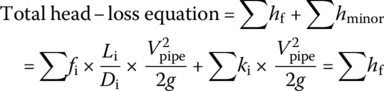
where
- hf is friction headloss (m)
- hminor is the component headloss (m)
Pump power can be calculated as follows to quantify energy footprint of a pump:
where
- P is power (W)
- γ is specific weight of water (N/m3)
- Q is flow rate (m3/s)
- hL is total headloss (m)
8.6.2 Pump Station
In pump station design, the net positive suction head available (NPSHavailable) must be greater than the net positive suction head required (NPSHrequired) to prevent cavitation of the pump. Otherwise the pressure will create implosions in the pump and decrease pump efficiency. The optimal guideline is to have at minimal 5–10% NPSHavailable greater than NPSHrequired. The basic equation to satisfy to prevent cavitation of pump is as follows:
where
- Ps/γ = suction head of the system
- Pv/γ = vapor pressure head of the pump
The best way to avoid cavitation would be to increase source pressure, raise the elevation of the source reservoir, and lower the elevation of the pump inlet. Otherwise, different pumps have to be selected to prevent cavitation of the pump.
For the pump and system to operate under steady conditions, pump total delivery head TDHtot will have to equal the headloss in the system, as characterized by the system curve. That equality is satisfied under the conditions where the TDHtot curve intersects the system curve. The value of Q at the operating point indicates the flow rate through both pumps and the piping. The head added by the original pump is the value of TDHorig at that Q, and the head added by the pump which would have the value of TDHboost at that Q.
8.7 Solar Energy
Solar energy is the only natural force that can reverse the entropy from disorder to order through photosynthesis. For this reason, green infrastructure (GI) plays a critical role in designing and building sustainable communities in regenerative way through harvest of solar energy using photosynthesis. Fundamentally, GI could increase production of primary biomass critical in the ecological system. It prevents pollution, adsorbs wastes, assimilates nutrients, and produces primary biomass by solar energy (Figure 8.22).

Figure 8.22 Simplified representation of energy and material flows across the biosphere and the economic system.
8.7.1 Calculation Solar Energy
In designing zero energy residential houses, solar energy and biogas are two major sources. Therefore, how much energy is needed and how much solar energy could be harvested are the critical design problems that are illustrated by the following examples as provided in Solar Photovoltaic Systems Technical Training Manual developed by the UNESCO (Wade, 2003).
8.7.2 Solar‐powered WWTP
100% natural treatment of wastewater at a treatment plant by John Todd at Ecological Design known as the Eco‐Machine. The OCSL building is powered by solar and geothermal power. Unlike other WWTPs, the OCSL does not use chemicals to treat the water, but a combination of microorganisms, algae, plants, and gravel and sand filtration to clean sewage water and return clean drinkable water back to the aquifer. Environmental sustainability, green energy, and regenerative design are the key. All the wastewater from toilets, sinks, and showers on the Omega campus feeds into storage tanks that collect human waste. The wastewater is then sent to the Eco‐Machine and is fed to “microscopic algae, fungi, bacteria, plants, and snails.” The first stage is two 5000‐gal anoxic tanks located underground and microbial organisms use the wastewater digest carbon, ammonia, phosphorus, nitrogen, potassium, and many other substances in the water. Water then flows to four man‐made wetlands behind the OCSL building. The wetlands use microorganisms and native plants such as cocktails and bulrushes to reduce biochemical oxygen demand, odorous gases, and nutrients such as ammonia and phosphorus. As the wastewater flows through the wetlands, the microorganisms and plants are fed. After that, there is a 75% increase in water’s clarity and a 90% reduction in its odor. The aerated lagoons are divided into four cells, each 10 feet deep. Without soil, beautiful tropical plants thrive here. The plants live on metal racks and their roots extend up to 5 ft into the water. The roots of the plants act as a habitat for the organisms in the lagoon and are sustained by them. After the lagoons, the water moves back outdoors to a sand filter; after which it reaches the standards for treated water. The treated water irrigates Omega’s parking lot where it infiltrates into the groundwater table. As it trickles down to the aquifer that sits 250–300 ft below, campus water is further purified as it is withdrawn from deep wells that tap the aquifer; the water is used in sinks, toilets, and showers. Naturally the used water is reclaimed with the Eco‐Machine at OCSL, and the purified water is released back to the aquifer, where the process can begin again. This full‐circle process makes the Eco‐Machine incredible and is an inspiration to interconnectedness utilizing processes to meet human’s needs.
8.8 Exercise
8.8.1 Questions
- In a typical WWTP, how is high‐grade energy such as electricity degraded to mechanical, chemical, and biological energy? Please quantify these energy in kWh/m3.
- What is embodied energy? Why there is an optimality between the embodied energy and operation energy consumption?
- How do thermodynamic laws dictate energy recovery in WRRF? Please analyze how energy could be recovered from chemical and biological to electrical energy. What is the unit energy production rate in kWh/m3 during each major process?
- In a typical WRRF, how much energy could be recovered in terms of theoretical energy contained in a typical wastewater sample of COD 500 mg/l and BOD 350 mg/l?
- Where is the optimal point for operation cost versus equipment size?
- What is the 10‐percentile unit energy benchmark for each process in WWTP?
- How large is the roof area needed for a typical house in Miami, Florida, to achieve net zero energy design by using 40‐W solar panels?
8.8.2 Calculation
- For three Miami‐Dade WWTPs of 300 MGD average flow rate, how much energy contained in average concentration of 330 mg/l COD and 223 mg/l BOD energy in theory if CO2 is reduced to CH4 or H2, respectively? If only biological fraction is able to be reduced to CH4, what are the maximal amount of energy that could be recovered in theory? If a typical theoretical value of energy content is about 1.75 kWh/m3, how is your estimate compared with this value?
- If all the WWTPs are to recover energy BOD from anaerobic digestion and the biogas produced is to generate electricity with 25% efficiency through combustion engine or to generate electricity through fuel cell with 40% efficiency, what are the percentages of self‐sustaining electricity if the plant needs 0.39 kw/m3 to operate? Please list any assumptions that you would in terms of conversion efficiency.
- If electricity costs $ 0.1/kWh, what would be the annual electricity bill for the operation of three WWTPs with the above energy recovery systems?
8.8.3 Project
8.8.3.1 Xiongan Project
- Xiongan has very ambitious plan to use 100% renewable energy. One of the unique energy in Xiongan is geothermal energy. Please collect necessary data, and estimate how many billion watts of energy could be extracted annually from geothermal energy with commercially available technologies.
- Energy efficiency is critical for energy‐positive plants. For 1, 2, and 5 million populations in 5, 10, and 20 years, respectively, please develop the most energy‐efficient WWTP process alternatives.
- Please estimate the total energy saving in billion watts if all the WWTPs in Xiongan is at minimal energy neutral.
8.8.3.2 Community Project
Please contact the plant manager of WWTP of your local city, and request energy consumption for each process of the plant and actual flow rate associated with energy consumption:
- Please conduct energy auditing at the WWTP: The energy consumption of each unit process should be divided by the actual flow rate.
- Please compare the unit energy consumption rate in MJ/MGD with the benchmark data provided in this chapter.
- Rank the performance of each unit process by percentage.
- Identify the biggest potential in energy efficiency improvement.
- Recommend different retrofitting methods to improve unit process energy efficiency.
References
- Ayres, R.U. and Kneese, A.V. (1969). Production, consumption and externalities. The American Economic Review 59: 282–297.
- Gans, N., Mobini, S., and Zhang, X. (2007). Mass and energy balances at the Gaobeidian wastewater treatment plant in Beijing, China. http://www.chemeng.lth.se/exjobb/E458.pdf (accessed 16 January 2018).
- Georgescu‐Roegen, N. (1971). The Entropy Law and the Economic Process. Cambridge, MA: Harvard University Press.
- Hammond, G.P. and Winnett, A.B. (2009). The influence of thermodynamic ideas on ecological economics: an interdisciplinary critique. Sustainability 1: 1195–1225.
- Howe, K.J., Hand, D.W., Crittenden, J.C. et al. (2012). Principles of Water Treatment. New York: Wiley Blackwell.
- Jonasson, M. (2007). Energy benchmark for wastewater treatment processes – a comparison between Sweden and Austria. Master thesis, Lund University.
- Krysiak, F. (2006). Entropy, limits to growth, and the prospects for weak sustainability. Ecological Economics 58: 182–191.
- Mizuta, K. and Shimada, M. (2010). Benchmarking energy consumption in municipal WWTPs in Japan. Water Science and Technology 62 (10): 2256–2262.
- Nouri, J., Jafarinia, M., Naddafi, K. et al. (2006). Energy recovery from wastewater treatment plant. Pakistan Journal of Biological Science 9 (1): 3–6.
- Pearce, D.W. and Turner, R.K. (1990). Economics of Natural Resources and the Environment. Baltimore, MD: Johns Hopkins University Press.
- Perrings, C. (1986). Conservation of mass and instability in a dynamic economy‐environment system. Journal of Environmental Economics and Management 13(3): 199–211.
- Stasinopoulos, P., Smith, M., Hargroves, K. and Desha, C. (2008). Whole System Design: An Integrated Approach to Sustainable Engineering. Earthscan: The Natural Edge Project.
- Tarallo, S., Shaw, A., Kohl, P., and Eschborn, R. (2015). A Guide to Net‐Zero Energy Solutions for Water Resource Recovery Facilities. Alexandria: Water Environment Research Foundation.
- Van Gool, W. (1992). Exergy analysis of industrial processes. Energy 17: 791–803.
- Wade, H.A. (2003). Solar Photovoltaic Systems Technical Training Manual, the UNESCO the United Nations Educational. Bangalore: Scientific and Cultural Organization.