11
Separation
Dispersion of wastes is ignorant of their value.
11.1 Principle 8
Separation may serve different purposes for reuse, recycle, and treatment. For solid waste, food waste (FW) should be separated from other waste because energy could be recovered from the FW. Papers and plastic separated from the solid waste stream could be reused or recycled. For zero water design, it is critical to separate blue (surface and groundwater), green (rainwater), gray (bath and laundry), and black (toilet water). Black water can be further separated into brown (urine) and black (feces). In developing countries, separated urine and feces toilets are promoted by many United Nations programs. N and P could be recovered from the concentrated urine, while anaerobic digestion of feces could generate methane and good organic fertilizer. In developed countries, waterless urinals could save significant amounts of tap water and reduce discharge to the sewer system. As a result, the design criteria of flow rate could be reduced due to water saving by waterless urinals. Separation also holds the key to sludge dewatering and disposal. Water as the final product in WWTP should be separated from any waste produced during the processes such as physicochemical treatment (coagulation) or biological treatment (activated sludge). The former needs to avoid adding chemicals, and the latter needs to separate organic content from water at the front end of a treatment systems. Enhanced separation of organic from wastewater (WW) using a cloth microsieving before WW enters the aeration tank prevents free water from being fixed as cellular water as part of activated sludge. The cloth microsieved solids could be directly diverted to the anaerobic digester to generate more methane to achieve energy‐positive WWTP. As a result, organic loading to the aeration tank would be reduced, and major secondary waste such as activated sludge would also be reduced significantly.
Separation plays important role in reuse, recycling, or treatment. For example, cardboard separated from domestic solid waste (DSW) stream could be used for cardboard reproduction. Fat–oil–grease (FOG) separated from kitchen waste could be codigested with sludge to generate more methane as shown in Table 11.1.
Table 11.1 Separation for different media and purposes.
| Media | Problems | For reuse | For recycle | For treatment |
| Air | Hazardous waste incineration | CO2 sequestration | Hazardous waste such as acid and base recycle | Catalyst |
| Water | Leachate combined with WW | Dripping irrigation | Nutrients | BMR, MF, NF, RO |
| Land | Food wastes | Kitchen oil for biodiesel | Fat, oil, and grease (FOG) codigestion with sludge | Compositing |
| Ecological | Invasive plants and aquatic species | Isolate and destroy the invasive plants and aquatic species |
As a treatment strategy, separation technologies are largely dependent on particle size. The particle size is an important factor in the process of water and wastewater treatment (WWT) in the past. Figure 11.1 shows the approximate range of particle size for each specific separation technology.
Figure 11.1 Particle size versus treatment technologies.
Figure 11.1 lists sizes for typical particulates in water: viruses, humic acids, clay/silt, bacteria, algae, and sand. Nutrients can be considered to be in the molecules category, with 10−10 m of atomic size. Reverse osmosis can essentially treat all different elements in the figure by allowing water filter through its membrane. One of the major design faults is that tank processes were specifically designed for specific range of particles, coagulation of colloidal particles, and sedimentation for flocculated matters. In WWT, however, different sizes of organic matters ranging from 10−3 to 1 mm could be separated in one unit process such as cloth microsieving. Depending upon the opening of the microsieves, 40–60% of organic pollutants could be diverted to anaerobic digester to produce biogas instead of producing sludge. The process would reduce aeration and sludge as secondary waste, and produces more methane for energy‐positive design.
11.2 Challenges and Opportunities
Domestic wastewater (DWW) constitutes 70% of WW in China. With an annual WW volume of 750 million m3, cumulative pollution contributed 225 million tons of COD to Chinese water bodies from 1992 to 2007 (Yu et al., 2015). In rural China, the major pollution sources are DWW and agricultural runoff. From 2001 to 2010, annual discharge of TN was 0.446 and 2.2 million tons and TP 80 000 and 230 000 tons from DWW and the agriculture in China, respectively (Guan et al., 2014). The major challenges faced by rural WWTP are a long construction period, high operation and maintenance (O&M) cost, low technical reliability of a complicated process, high O&M costs, low recycling rates of plants, and geological conditions requiring different designs. More importantly, there are no sustainability design guidelines for rural WWTP and sludge disposal for increasing WW flow rate due to rapid urbanization and population growth.
To solve these urgent WWT challenges, separation is one of the most effective ways to remediate the deterioration of water quality in rural China. There are many opportunities for separation in China. WWT in rural areas of China could be the last big market where only 22% of WW has been treated. China has about 280 000 villages within 1 805 counties, but the WWT rate in rural China is only 13%. In Northern China, groundwater is the major drinking water resource. If WW is not properly treated, contamination of groundwater will spread widely. The 13th Five‐Year Environmental Plan for rural China requires one‐third of villages to have WWT facilities. Currently, 160 million farmers do not have WWT. If $1400 of capital cost for WWT was required for each rural resident, the market capital to build WWT facilities alone would be $240 billion. Indeed, the WWT capital market for rural China could increase exponentially to 3.5, 12, and 20 billion USD in 2016, 2020, and 2025, respectively. In the next decade, the market for WW treatment and the sewer pipe network in China is estimated at 300 billion USD. Separation of gray water from black water would decrease WW at minimal by half. The separated gray water could be used for irrigation of green infrastructures such as wetlands. Separation of urine from feces may offer a way to recover N and P. For example, Ishii and Boyer (2015) used the following unit values in their calculation of urine separation project for a dormitory at the University of Florida (Table 11.2).
Table 11.2 Unit values for urine separation design.
| Unit values for urine separation design | |||
| Human consumption | Air | 28 | m3/day |
| Water | 1.5 | kg/day | |
| Food | 1.5 | kg/day | |
| Calories | 2000 | cal/day | |
| Flash | Urine | 0.05 | l/day |
| Feces | 6 | l/day | |
| Total volume | Urine | 0.2 | l/day |
| Feces | 0.5 | kg/day | |
| Cost | Water from groundwater | 0.917 | $/m3 |
| WW treatment by central WWTP of 20 000 PE | 1.336 | kWh/m3 | |
| Electricity | 0.1 | $/m3 | |
| Energy composition in the United States | Coal | 50 | % |
| Natural gas | 20 | % | |
| Nuclear | 20 | % | |
| Renewable | 10 | % | |
| Nutrient removal efficiency | N | 84 | % |
| P | 49.8 | % | |
| Waterless urine toilet | 700 | $ | |
| Regular urine toilet | 200 | $ | |
According to the assumptions of Table 11.2, for 8 823 population equivalent (PE) annually, the total N and P that can be recovered from 1 920 m3 of urine is 13 200 and 1 020 kg, respectively.
In the past, China designed and built conventional systems such as activated sludge as the major process for towns of more than 1000 people. However, high energy consumption and large amounts of sludge prevent the normal operation of the WWTPs built in recent decades. Two likely extremes exist in rural markets: the technologies were either too low tech and resulted in not enough protection of water resources or too high tech, such as membrane biological reactor (MBR). Unfortunately, a major difficulty also arises due to high capital cost and the intensive energy required to run. As a result, the unit operating cost might be as high as one USD per cubic meter of WW treated. With limited resources of rural WWTP, many of these plants will most likely run into financial difficulty. For these reasons, decentralized and energy positive WWTPs are critical to ensure sustainable WW management in rural China.
In urban China, activated sludge processes have been utilized in more than 95% of the WWTPs in the past four decades. However, most of the WWTPs do not have sludge treatment facility due to the cost of intensive energy. In 2015, cities and counties had a total of 3717 WWTPs with a treatment capacity of about 157 million cubic meters/day. The total treatment capacity of sewage is 48.06 billion cubic meters per year, with 84.1% operating load rate. However, sludge treatment and disposal facilities were only 43.4% at the end of 2013, because sludge treatment and disposal was not mandatory for WWTPs by law. The 12th Five‐Year Plan (FYP) requires the disposal rate of sludge treatment to be 80% by the municipalities directly under the central government, the provincial capitals, and the cities to reach 70% while 30% is required for cities at county or township levels. With consideration of energy footprints and the energy‐positive unit process in WWTP, only 60 of 3717 WWTPs in China have anaerobic digestion facilities of sludge, which is barely 1.7% of the total WWTPs in China. Therefore, it is estimated that sludge treatment and disposal market could be as high as 50 billion USD in the next 10 years. The major sludge disposal problem is the optimization of sludge digestion technology. For example, various composting technologies need to be improved. Sludge heat drying and incineration technology and equipment should be integrated. Land application of treated sludge needs to be monitored. Although incineration, carbon char, and landfill are different options, the land application of anaerobic digested sludge should be the future direction due to the energy production as biogas and pathogen‐free organic fertilizer sludge. According to the US experience, treatment strategy depends upon the PE. To effectively and economically meet discharge standards, three scales are residential, community, and city as shown in Table 11.3, which lists the most suitable treatment technologies and the operation parameters and performance levels required in the United States.
Table 11.3 Operating parameters and key performance metrics in the United States.
| Parameter | Household | Community | City |
| Wastewater treatment standard | Secondary biological treatment for subsurface drip irrigation reuse | Advanced treatment with nitrogen removal for surface water discharge and reuse | Advanced biological treatment for reuse and deep well injection |
| BOD5 in treated effluent(mg/l) | 30 (20–40)a | 1.8 (0.8–3.5) | 2.1 (1.2–2.4) |
| Percentage of water reclaimed (%) | 100 | 77 | 56 |
| Effluent TN to soil from reclaimed water (mg/l) | 16 (2–31) | 0.23 (0.03–6.8) | 2.3 (1.3–3.1) |
| Effluent TP to soil from reclaimed water (mg/l) | 0.16 (0.12–0.20) | 0.005 (0.004–0.04) | 0.01 (0.004–0.03) |
| Total biosolids production (kg/year) | 9.8a | 60 000 | 2 894 136 |
Note: Numeric values presented are average values, where values in parentheses are minimum and maximum values.
Separation technologies are considered as phase transfer methods and do not destroy organic pollutants. Nevertheless, precipitation, coagulation, flocculation, and sedimentation are still very important unit processes in treating toxic wastewater containing metals. For water reuse, micro-filtration, nano-filtration, and reverse osmosis are critical to ensure the effluent water quality to meet the water reuse standards.
11.3 Precipitation
Chemical precipitation of metal‐contaminated water has long been used in treating WW from industrial applications, such as metal finishing and plating. Effective precipitation is usually accompanied by coagulation, flocculation, and clarification and/or filtration to separate the solid and liquid phases of the waste stream by raising the pH of the solution to lower the metal solubility. Alkali‐precipitating agents such as caustic soda (NaOH), hydrated lime (Ca(OH)2), and magnesium hydroxide (Mg(OH)2) are common precipitating agents. The solubility of metal hydroxide precipitates decreases with increasing pH to a minimum value called the isoelectric point. Chemical precipitation depends on several variables:
- Maintenance of a proper pH range throughout the precipitation reaction and subsequent settling time.
- Addition of a sufficient excess of treatment ions (precipitating agent) to drive the precipitation reaction to completion.
- Effective removal of precipitated solids.
Figure 11.2 is a typical schema of a metals treatment system.
Figure 11.2 Continuous metal precipitation, coagulation, and flocculation (P/C/F) system.
After precipitation, coagulation and flocculation are required to destabilize colloidal particle and to grow the particle so that they can settle from WW.
11.4 Coagulation and Flocculation
Coagulation destabilizes colloidal particles, while flocculation refers to growth of destabilized colloidal particles. The stability of colloidal particles is defined by the size, area, and charge of the surface. Colloidal particles attract one another through van der Waals forces and have repulsion forces going against one another due to the zeta potential. When suspended in water, the charge on organic and inorganic colloids is typically negative. Flocculation is the process of bringing together the destabilized or “coagulated” particles to form a larger agglomeration of floc by physical mixing or addition of chemical coagulant aids or both. Electric double layer (EDL) refers to a fixed and a diffusing layer. The potential voltage from the shear of a plane is called the zeta potential. Destabilization reduces the zeta potential. Commonly used coagulants include AlCl3 (alum), which might cause Alzheimer’s disease due to residual alum. FeCl3 and FeSO4 (ferric ion) are a better choice than alum. The rate of flocculation depends upon several factors: (i) the nature of the particle surface, (ii) the presence of charges, (iii) the shape of the particles, and (iv) the density of the particles. Jar tests are used to determine the dose of coagulants through experiment (Figure 11.3).
Figure 11.3 Mechanisms of coagulation and flocculation.
Mixing provides greater uniformity of the WW feed and disperses precipitating agents, coagulants, and coagulant aids throughout reactor to ensure the most rapid precipitation reactions and subsequent settling of the precipitates. To quantify the degree of mixing, the following factors must be considered: (i) the amount of energy supplied, (ii) the mixing residence time, and (iii) the related turbulence effects of the specific size and shape of the tank. For mechanically stirred mixing basins, G can be calculated as follows:
where
- P = power applied to stirring, W (ft‐lbf/s = HP × 550)
- V = reactor volume m3 (ft3)
- μ = dynamic viscosity N‐s/m2 (lbf‐s/ft2)
Power requirements are determined from
where
- P = power applied to stirring, W (ft‐lbf/s)
- CD = coefficient of drag
- A = paddle area, m2 (ft2)
- ρ = fluid density, kg/m3 (slugs/ft3)
For water at 20°C,
where v is the relative velocity of paddles in fluid (m/s [fps]), typically about 0.6–0.75 of paddle tip speed.
11.4.1 Camp–Stein Equation
Velocity gradient provided by the mixer can be estimated by the Camp‐Stein equation:
where
 = power dissipation (mixer power transferred to bulk fluid)
- V = volume of reactor
- μ = dynamic viscosity
After coagulation of the rapid mixing stage, flocculation is based on slow‐to‐enhance contact between particles to promote the growth of destabilized floc. Under the hydraulic force, G, the orthokinetic flocculation colloid number rate decreases according to the following equation:
In‐line static mixers are a type of pipe reactors used for rapid mixing that can be done for any type of flow (laminar, transitional, and turbulent). When comparing both the static and tank mixed reactors, more energy is required in the tank than in the static mixer.
11.4.2 Static and Plug‐flow Reactor Mixers
Figure 11.4 shows the hydraulic characters of PFR, Batch, and CSTR reactors.

Figure 11.4 Concentration profile for different reactors.
11.4.3 Power, Pressure, and Pump in Reactors
Hydraulic power formula is used to calculate the power of each reactor:
where
- γ = specific gravity
- Q = flow rate
- hL = headloss
Tank reactors form dead zones and short‐circuiting, whereas plug‐flow conditions minimize short‐circuiting and completely avoid dead zones. The US EPA Design Manual (2004) provided good design examples of separation technologies.
Figure 11.5 Titration curve for pacification of chromium waste. Figure 11.6 Titration curve for neutralization of waste following chromium reduction. Figure 11.7 Column testing results. Figure 11.8 Solubility of metal hydroxides and sulfides as a function of pH (US EPA, 1980).

After precipitation, sludge handling is an energy‐intensive process. Typically, sludge from water treatment plants is pressure filtrated since it is often difficult to dewater, particularly alum sludge and softening precipitates containing magnesium hydroxide. Gravity‐thickened alum waste is conditioned by the addition of lime slurry. The conditioned sludge is then fed continuously to the pressure filter until filtrate ceases, and the cake is consolidated under high pressure. Filtrate is measured through a weir tank and recycled to the inlet of the water treatment plant. The cake is transported by truck to a disposal site. Alum sludge is conditioned using lime and/or fly ash. Lime dosage is in the range 10–15% of the sludge solids. Ash from an incinerator, or fly ash from a power plant, is applied at a much higher dosage, approximately 100% of dry sludge solids. Polyelectrolytes may also be added to aid coagulation. Fly ash and diatomaceous earth are used for precoating; the latter requires about 50.2 kg/m2 of filter area. Under normal operation, cake density is 40–50% solids and has a dense, dry, textured appearance. Alum sludge from surface water treatment is amenable to centrifuge dewatering to about 20% solids. The removal efficiency in a scroll centrifuge ranges from 50 to 95% based on operating conditions and polymer dosage. Alum sludge from surface water coagulation settles to a density in the range of 2–6% solids. Coagulation‐softening mixtures from the treatment of turbid river waters gravity‐thicken approximately as follows: alum–lime sludge, 4–10%; iron–lime settlings, 10–20%; alum–lime wash water, about 4%; and iron–lime backwash, up to 8%. The density achieved in gravity thickening relates to 8%. Lime‐softening precipitates compact more readily than alum floc in a scroll centrifuge. A settled sludge input with 15–25% solids can be dewatered to a solidified cake of 65%. Suspended solids recovery is often 85–90% with polyelectrolyte flocculation. The performance of thickener handling water treatment plant waste varies with the character of the water being treated and the chemicals applied. Calcium carbonate residue from groundwater softening consolidates to 15–25% solids. Solids content and sludge volume are intrinsically linked as in Table 11.4 and Figures 11.9 and 11.10.
Table 11.4 Density and volume of sludge.
| Sludge solids content (%) | kg sludge/kg dry solids | m3 sludge/ton dry solids |
| 1 | 100 | 100 |
| 2 | 50 | 50 |
| 5 | 20 | 20 |
| 10 | 10 | 9.7 |
| 15 | 6.7 | 6.4 |
| 20 | 5.0 | 4.7 |
| 30 | 3.3 | 3.0 |
| 40 | 2.5 | 2.2 |
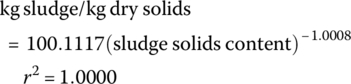
Figure 11.9 kg sludge/kg dry solids versus sludge solids content (%).

Figure 11.10 m3 sludge/ton dry solids versus sludge solids content (%).
The regression equation between the log(kg sludge/kg dry solids) and the log(sludge solids content) is
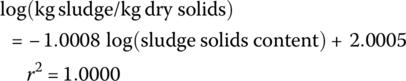
or
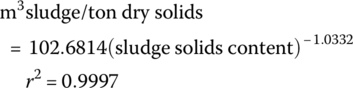
The regression equation of log(m3 sludge/ton dry solids) and log(sludge solids content) is
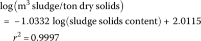
or
11.5 Membrane Filtration Systems
Water membrane filtration systems can be classified as (i) microfiltration, (ii) ultrafiltration, (iii) nanofiltration, (iv) reverse osmosis, and (v) biomembrane reactors. All of these separation technologies are designed to filter a specific range size particle with the corresponding pore size. For example, microfiltration focuses on the largest particle as shown in Figure 11.1. Reverse osmosis is to remove the smallest particles such as ion in the size ranging from several angstrom due to the small membrane pore sizes. It removes cations, acids, and salts at angstroms to nanometers. The filtration systems usually remove the large size particles first. Therefore, microfiltration and ultra‐filtration are typically used for pre‐treatment for nanofiltration or reverse osmosis to prevent fouling.
For water treatment or reclaiming treated wastewater, high pressure is required to force water passing through membrane as permeate and leave concentrate as waste by‐product. Pressure through the pump to aim for permeate performance using hollow fibers is
This is the formula to determine the pressure of the flow.
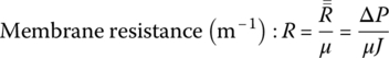
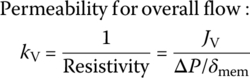
where: ΔP = transmembrane differential pressure, psi or kPa
dynes/cm2
J = flux, gfd or Lmh
kv = Permeability for overall flow
μ = viscosity constant of water
δmem = thickness of the membrane, ft or m
The Long Term 2 Enhanced Surface Water Treatment Rule (LT2ESWTR) requires state to report integrity test of membrane filtration system to earn credit for virus removal (US EPA 2005). The procedure is described in the Membrane Filtration Guidance Manual (US EPA, 2005). Example 11.2 illustrates how to calculate the required technical values to comply with the EPA’s requirements for membrane filtration to earn 3 log virus removal credit. The system is a submerged vacuum-driven hollow-fiber membrane. The upper control limit (UCL) refers to the maximal pressure before the membrane is breached. Log removal value is defined as the log Ceffluent – log Cinfluent.
11.6 Activated Carbon Adsorption
Activated carbon has large adsorption surface area and is easy to design and operate. Therefore, it has been widely used in industrial wastewater treatment. The design is based upon column test results as shown in Example 11.3.
Table 11.5 Design data. Figure 11.11 RDX concentration versus bed volumes. Table 11.6 Pilot plant data. Table 11.7
CalgonCarbon® manufacturer’s data of Model 12‐40. Figure 11.12 Air stripper system. Table 11.8 Freundlich isotherm table for this specific carbon with given K and 1/n values at 77°F.
Design data
Flow rate
50
l/s
Contaminant concentration influent
69
µg
Contaminant concentration effluent
4
µg

Pilot plant data
Carbon sample
XYZ
Carbon company
Column inside diameter
108
mm
Column area
9150
mm2
Bed volume
5.56
l
Flow rate
2.84
l/min
Hydraulic loading
310
lpm/m2
Bed depth
0.61
m
EBCT (each column)
2
min
RDX influent concentration
69
µg/l
Weight of GAC per column
2.32
kg
Weight of RDX per column
14.2
g
Run time
150
days
CalgonCarbon® manufacturers
Model 12‐40
Diameter
3.66
m
Depth
3.35
m
Carbon per adsorbent
18180
kg
GAC density
420
kg/m3
Contaminant
K
C (lb/in2)
1/n
x/m
PCE
1.4
0.0001905
0.156
0.367952
TCE
1.4
0.0001778
0.23
0.192138
Benzene
1.1
0.0001143
0.131
0.334963
Toluene
0.7
0.0000635
0.111
0.239445
11.7 Anaerobic Membrane Biological Reactor
Bioreactor eliminates BOD and nutrients through either aerobic or anaerobic processes. Anaerobic digestion is a key technology in recovering biogas from sludge. The primary treatment is to remove the suspended solids, the secondary treatment is to degrade BOD, and the tertiary treatment is to remove nutrients. MBR combines the secondary and tertiary treatment together. It could remove both BOD and significant portion of nutrients due to longer solid retention time of large biomass in the MBR. Table 11.9 lists the advantages of membrane bioreactors.
Table 11.9 Advantages and disadvantages of membrane bioreactors.
| Advantages | Disadvantages |
| Small footprint | Aeration limitation |
| Complete solid removal | Membrane fouling |
| Effluent disinfection | Membrane costs |
| Removal of organic, nutrient, and solid | High operating costs |
| High loading rate capability | |
| Low/zero sludge production | |
| Rapid start‐up | |
| Sludge bulking not a problem | |
| Modular/retrofit |
A typical layout of MF within a treatment plant is as follows (Figure 11.13).
Figure 11.13 Aerobic biological treatment with membrane separation.
Figure 11.14 Submerged membrane bioreactor.
According to the different arrangement of membrane bioreactors, they can be classified as submerged MBR (Figure 11.14) versus MBR sidestream (Figure 11.15).
Figure 11.15 External membrane bioreactor.
Within the MBR, one of the most popular membranes is the hollow‐fiber MBR (Figure 11.16).
Figure 11.16 Hollow‐fiber membrane bioreactor.
According to loading rate to anaerobic reactors, low and high rates of AD are classified as follows (Table 11.10).
Table 11.10 Low‐ and high‐rate anaerobic digesters.
| Low‐rate anaerobic reactors | High‐rate anaerobic reactors | |
| Type | Anaerobic pond Septic tank Imhoff tank Standard rate anaerobic digester |
Anaerobic contact process Anaerobic filter (AF) Upflow anaerobic sludge blanket (UASB) Fluidized bed reactor Hybrid reactor: UASB/AF Anaerobic sequencing batch reactor (ASBR) |
| Characteristics | Slurry‐type bioreactor, temperature, mixing, SRT, or other environmental conditions are not regulated. Loading of 1–2 kg cod/m3‐day | Able to retain very high concentration of active biomass in the reactor Thus extremely high SRT could be maintained irrespective of HRT. Load 5–20 kg cod/m3‐day Cod removal efficiency: 80–90% |
Using the volumetric organic loading rate, which is in kg COD/m3‐day, the volumetric organic loading rate can be calculated as follows:
where
- VOLR = volumetric organic loading rate (kg COD/m3/day)
- So = wastewater biodegradable COD (mg/l)
- Q = wastewater flow rate (m3/day)
- V = bioreactor volume (m3)
where
H= reactor height (m)
θa = allowable hydraulic retention time (h)
Q = wastewater flow rate (m3/h)
A = surface area of the reactor (m2)
For dilute WW with COD < 1000 mg/l,
The Long Term 2 Enhanced Surface Water Treatment Rule (LT2ESWTR) requires state to report integrate test to earn credit for virus removal (US EPA 2005). The procedure is described in the Membrane Filtration Guidance Manual (US EPA, 2005). Example 11.5 illustrate the calculation on how to calculate the required technical values to earn the 3 log virus removal credit for a submerged vacuum-driven hollow-fiber membrane.
11.8 Air Stripping
Air stripping is a common process used to remove VOCs from water. This is achieved by enabling contact between the liquid (in this case water) and gas (air). Gas is treated to remove the VOCs before it is released into the atmosphere. Air stripping involves the mass transfer of VOCs dissolved in water from the contaminated water to the air phase. This principle is known as Henry’s law:
where, at equilibrium, Pa is the partial pressure of a gas above a liquid and is proportional to the mole fraction of the gas dissolved in the liquid, Xa. Ha is the known Henry’s constant for the gas.
Thermal oxidation and activated carbon are typically used to treat off‐gas that exceeds regulation limits. Thermal oxidation eliminates the contaminant but is a costly, complex process. Low‐profile air strippers can remove 99% of most VOC contaminants. The efficiency of the stripper can be improved, and additional stripping incorporated by increasing the number of trays. Efficiency can also be increased by increasing the airflow. Sieve tray air strippers operate in a similar way to packed‐column air strippers. The difference is that the liquid (water) flows across trays that are perforated with small holes over a weir and through a downcomer to the next lower tray until the treated water flows from the bottom of the stripper. Gas (air) is bubbled through the holes in the trays, stopping the liquid from dripping through them. The VOCs are transferred from the liquid to the gas phase as the air is bubbled through the water on the trays. Figures 11.17 and 11.18 show a simplified diagram of a packed‐column and a low‐profile sieve air stripper.
Figure 11.17 Simplified diagram of a packed‐column air stripper.
Figure 11.18 Simplified diagram of a low‐profile sieve tray air stripper.
The theoretical number of trays required is estimated using the following relationship:
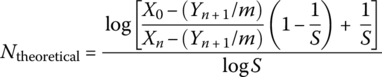
where
- X0 = concentration of contaminant (TCE) in the inlet water phase: 10 mg/l
- Xn = concentration of contaminant (TCE) in the treated water phase: 0.1 mg/l
- N = number of theoretical plates (assumes that the liquid on each plate is completely mixed and where that the vapor leaving the plates is in equilibrium with the liquid)
- H = Henry’s constant (kPa)
- m = slope of equilibrium curve (H/Pt)
- G = kg‐moles air/min
- L = kg‐moles of water/min
- Pt = ambient pressure (kPa)
- S = stripping factor
- Yn+1 = concentration of volatiles in the air entering the air
For air stripping Yn+1 = 0 (the concentration of TCE in the air entering the air stripper is zero), and the equation becomes

A packed‐column air stripper consists of a cylindrical column that contains an open‐structured packing material. Water containing the VOCs enters the top of the column and flows down through packing material. At the same time, air flows up through the column (countercurrent flow). As the water and air pass each other, the VOCs are transferred from the water phase to the air phase. The water phase leaves the bottom of the column with most of the VOCs removed. The VOCs that are in the air phase exit from the top of the column. For the packed‐column air stripper, the mass balance equation for VOCs in the liquid versus gas phases is as follows:
where
- L = molar liquid (water) flow per unit of stripper cross‐sectional area

- G = molar gas (air) flow per unit of stripper cross‐sectional area

- xai = mole fraction of contaminant in liquid (water) influent
- xae = mole fraction of contaminant in liquid (water) effluent

- yai = mole fraction of contaminant in gas (air) influent
- yae = mole fraction of contaminant in gas (air) effluent

If influent air is not contaminated by VOC, the molar ratio of gas (air) to liquid (water) is
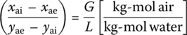
where
- xai and L = field measurements and xae imposed by ARAR
- pTe = total pressure of gas (air) effluent (atm)
- Pae = partial pressure of contaminant a in gas (air) effluent (atm)
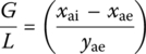
From Dalton’s law of partial pressures,

At equilibrium from Henry’s law,
Figure 11.19 Cross‐sectional area of perforated plate section. Figure 11.20 Random “dumped” packed tower. Table 11.11 Contaminants. a The [gram] molecular weight of the contaminant. b Ha at 20°C (296.13 K). Table 11.12 Background inorganic concentrations. Note: a GEqW is the [gram] equivalent weight of the inorganic ion. Table 11.13 Removal requirements. Table 11.14 Critical contaminants. Table 11.15 Water at 20°C (293.16 K). Table 11.16 Air at 20°C (293.16 K) and 1 atm. Table 11.17 Air stripping cost.

Contaminant
Formula
GMWa (g/g‐mol)
CAS number
Hab (atm/mol/mol)
Benzene
C6H6
78.11
71‐43‐2
309.2
Toluene
C6H5CH3
92.14
108‐88‐3
353.1
Trichloroethylene (TCE)
C2HCl3
131.50
79‐01‐6
506.1
Ion
mgl
GMW
Valence
GEqWa
meq/l
mg/l as CaCO3
CO2
0
44
−2
22
0.00
0.00
Anions
SO4
60
96
−2
48
1.25
62.46
Cl
54
35
−1
35
1.52
76.15
HCO3
30
61
−1
61
0.49
24.58
Total
163.19
Cations
Na
10
23
1
23
0.43
21.75
Ca
40
40
2
20
2.00
99.80
Fe
0.3
56
2
28
0.01
0.54
Mg
10
24
2
12
0.82
41.12
Mn
0.05
55
2
27
0.00
0.09
Total
163.29
Contaminant
Concentration (µg/l)
Mole fraction (mol/mol)
Influent, Cai
Standard, Cae
Removal requirement
Xai
Xae
Total VOCs
2500
NA
NA
NA
NA
Benzene
750
10
98.7%
0.17330
0.00231
Toluene
1000
100
90.0%
0.19588
0.01959
Trichloroethylene (TCE)
750
100
86.7%
0.10294
0.01373
For Pte = 1 atm and 20°C (296.13 K)
![]()
Contaminant
![]()
![]()
![]()
Benzene
0.9867
0.2320
4.253 m3/m3
Toluene
0.9000
0.2649
3.397 m3/m3
Trichloroethylene (TCE)
0.8667
0.3797
2.283 m3/m3
Critical contaminant (benzene)
![]()
The properties of the liquid (water) at 20°C
![]()
Liquid surface tension
![]()
Liquid viscosity
![]()
Liquid density
![]()
Nominal diameter
![]()
Total surface area
![]()
Critical surface tension for polyethylene packing
![]()
Packing factor
The properties of the gas (air) at 20°C (293.16 K) and 1 atm
![]()
Gas viscosity
![]()
Gas density
Flow rates (m3/s)
Flow rates (Mgal/year)
Low estimate cost (M)
High estimate cost (M)
0.01
83.32
3.3
14.2
0.1
833.183
33.3
141.6
1
8 331.836
333.3
1 416.4
11.9 LCA Tools for WWTPs
The core criteria in SEE design are the footprints of EEIS on energy and materials such as water, carbon, and nutrients according to its life cycle of the EEIS. To assess these footprints, many LCA tools have developed as shown in Table 11.18 (Figure 11.21).
Table 11.18 Life cycle assessment tools for WWTPs.
| Type | Description of methodology | Estimation tool | Tool format | Available | Applicable | Source |
| Process LCA‐based tools | Use process‐based inventory over life cyclea | SimaPro | Software | Commercial | Varies, any product or process | www.pre.nl |
| GaBi | Software | Commercial | www.gabi‐software.com | |||
| SiSOSTAQUA | Software | Commercial | www.simpple.com | |||
| Hybrid LCA‐based tools | Use both process‐based and input–output‐based inventory over life cycleb | WEST | MS‐Excel | Upon request | Water, water reuse, desalination | Dr. Jennifer Stokes at [email protected] |
| WWEST | MS‐Excel | Upon request | Wastewater | Dr. Jennifer Stokes at [email protected] | ||
| WESTWeb | Web based | Public | Water, water reuse, desalination wastewater | west.berkeley.edu | ||
| Specific tools | Uses input parameters specific to utility over O&M | Tampa Bay Waterc | MS‐Excel | Upon request | Water and desalination | www.tampabaywater.org |
| Johnston Toold | MS‐Excel | Upon request | Water | Dr. Tanju Karafil at [email protected] | ||
| Other related tools | Not specifically used to estimate emissions from water reuse or desalination facilities but contain aspects that are applicable | CHEApete | Web based | Public | Wastewater | cheapet.werf.org |
| UK Environment Agency toolf | MS‐Excel | Upon request | Water supply, water reuse, desalination | Environment Agency at [email protected] | ||
| Bridle and BSM2G toolg | Software | Public | Wastewater | Author Lluis Corominas at [email protected] | ||
| System dynamicsh | Software | Commercial | Varies | www.iseesystems.com | ||
| GPS‐Xi | Software | Commercial | Wastewater | www.hydromantis.com/GPS‐X.html | ||
| Carbon Accounting Workbook, 5th Versionj |
MS‐Excel | Commercial | Water | www.ukwir.org | ||
| mCO2k | Software | Commercial | Wastewater | www.mwhglobal.com | ||
| BioWin 4.0l | Software | Commercial | Wastewater | www.envirosim.com |
Sources:
Figure 11.21 Comparison of carbon footprint estimate using Tampa Bay Water and WESTWeb tools.
(Source: Cornejo et al. (2016). Reproduced with permission of American Chemical Society.)
Databases that could be used for LCA of WWTP include:
- E‐PRTR: 28 000 industry pollutants by EU Pollutant Release and Transfer (Yoshida, Water Research, 56, 292–303, 2014).
- International Reference Life Cycle Data System (ILCD) v2.2 USLCI (Eco‐invent Center, 2007; NREL, 2012).
- TRACI (Tool for Reduction and Assessment of Chemical and Other Environmental Impacts) (US EPA, 2014).
- IMPACT World+.
Separation strategy could be effective on different spatial scales because treated WW should be disposed approximate to the reuse. From a sustainability point of view, the energy footprint of WW treatment per cubic meter of WW on different spatial scales such as household (250 GPD), community (0.31 MGD), and city (10.3 MGD) decreases as shown in Figure 11.22 due to economy of scale.
Figure 11.22 Embodied energy of wastewater systems with collection, treatment, water reuse, and resource recovery offsets on different scales.
(Source: Cornejo et al. (2016). Reproduced with permission of American Chemical Society.)
For all the treatment strategies, water reuse is the major positive offset of energy footprint regardless of scale. In conventional AS process, electricity is the major factor contributing to energy consumption. Table 11.19 illustrates the contribution of construction and O&M phases to energy footprint on different scales.
Table 11.19 Percentage contribution from sewer collection, treatment, and water reuse to the total embodied energy of wastewater systems and resource recovery offsets on different scales.
Source: Cornejo et al. (2016). Reproduced with permission of American Chemical Society.
| Phase | Stage | Description | Household (250 GPD) | Community (0.31 MGD) | City (10.3 MGD) |
| Construction | Collection | Piping | — | 2.5% | 9.2% |
| Treatment | Tanks | 14.6% | 2.3% | 3.1% | |
| Reuse | Piping | 7.2% | 0.4% | 12.5% | |
| O&M | Collection | Electricity | — | 1.5% | 5.5% |
| Treatment | Sludge removal | 0.02% | 0.02% | 0.04% | |
| Chemicals | — | 6.3% | 17.5% | ||
| Electricity | 34.3% | 62.8% | 22.5% | ||
| Diesel | — | 2.4% | 5.5% | ||
| Reuse | Electricity | 43.8% | 17.9% | 15.4% | |
| Diesel | — | 3.9% | 8.9% | ||
| Resource recovery offsets | Potable water offsets | −17.9% | −15.4% | −25.2% | |
| Fertilizer offsets | −3.3% | −0.5% | −5.1% | ||
| Energy offsets | — | — | −18.5% |
To achieve sustainable design in rural areas, solar energy is the best way to reduce energy footprint by using constructed wetland. A decentralized WWT system utilizing constructed wetlands will be the major technology due to the relatively large residential area for the photo‐remediation or treatment of WW. Solar energy would significantly reduce electricity consumption and treat WW efficiently and economically.
11.10 Capital and O&M Costs of Membrane Filtration
There are three major cost categories: (i) Capital cost includes cost of the system and process reactors. (ii) Operation includes cost of operating the system. (iii) Maintenance covers the cost of fixing and keeping the system up to date. Operation and maintenance costs are generally referred as O&M cost in terms of percentage of capital cost.
Table 11.20 Capital cost and operation and maintenance cost of microfiltration at different flow rates. Table 11.21 Unit capital cost and unit operation and maintenance cost of microfiltration at different flow rates. Table 11.22 Unit cost ratio of microfiltration at different flow ratios. Figure 11.23 Unit capital cost/unit capital cost0 versus Q/Q0 for microfiltration, unit capital cost0 = 1145.77$/kgal, Q0 = 1 MGD. Figure 11.24 Unit capital cost/unit capital cost0 versus Q/Q0 for microfiltration, unit capital cost0 = 1145.77$/kgal, Q0 = 1 MGD. Figure 11.25 Unit O&M cost/unit O&M cost0 versus Q/Q0 for microfiltration, while unit O&M cost0 = 0.7963 $/kgal, Q0 = 1 MGD. Figure 11.26 Unit O&M cost/unit O&M cost0 versus Q/Q0 for microfiltration, unit O&M cost0 = 0.7963$/kgal, Q0 = 1 MGD. Table 11.23 Capital cost and operation and maintenance cost of reverse osmosis and nanofiltration at different flow rates. Table 11.24 Unit capital cost and unit operation and maintenance cost of reverse osmosis and nanofiltration at different flow rates. Table 11.25 Unit cost ratio of reverse osmosis and nanofiltration at different flow ratios. Figure 11.27 Unit capital cost/unit capital cost0 versus Q/Q0 for reverse osmosis and nanofiltration, unit capital cost0 = 2630.21$/kgal, Q0 = 1 MGD. Figure 11.28 Unit O&M cost/unit O&M cost0 versus Q/Q0 for reverse osmosis and nanofiltration, unit O&M cost0 = 7.4172$/kgal, Q0 = 1 MGD.
Q (MGD)
2006 capital cost ($)
2006 operation and maintenance costs ($/year)
1
1 145 772.56
290 645.63
2
1 751 658.86
315 291.25
4
2 967 431.47
361 582.50
6
4 181 204.09
410 873.75
8
5 395 976.70
457 165.00
10
6 611 749.31
503 456.25
20
12 685 612.37
742 912.50
40
25 372 224.74
1 230 825.00
60
37 520 950.86
1 706 737.51
80
50 208 563.23
2 194 650.01
100
62 356 289.35
2 670 562.51
Q (MGD)
Unit capital cost ($/kgal)
Unit O&M costs ($/kgal)
1
1145.77
0.7963
2
875.83
0.4319
4
741.86
0.2477
6
696.87
0.1876
8
674.50
0.1566
10
661.17
0.1379
20
634.28
0.1018
40
634.31
0.0843
60
625.35
0.0779
80
627.61
0.0752
100
623.56
0.0732
Q/Q0
Unit capital cost/ unit capital cost0
Unit O&M costs/unit O&M costs0
1
1.0000
1.0000
2
0.7644
0.5424
4
0.6475
0.3110
6
0.6082
0.2356
8
0.5887
0.1966
10
0.5771
0.1732
20
0.5536
0.1278
40
0.5536
0.1059
60
0.5458
0.0979
80
0.5478
0.0944
100
0.5442
0.0919

Q (MGD)
2006 capital cost ($)
2006 operation and maintenance costs ($/year)
1
2 630 207.84
2 707 281.79
2
3 958 402.454
2 851 711.803
4
6 527 627.349
3 146 977.202
6
8 979 523.093
3 440 332.766
8
11 383 885.71
3 734 517.654
10
13 735 967.79
4 027 219.037
20
25 229 374.62
5 496 830.50
40
47 430 550.07
8 430 904.35
60
69 181 992.93
11 362 030.64
80
90 719 913.20
14 291 757.49
100
112 104 198.19
17 216 045.49
Q (MGD)
Unit capital cost ($/kgal)
Unit O&M costs ($/kgal)
1
2630.21
7.4172
2
1979.20
3.9065
4
1631.91
2.1555
6
1496.59
1.5709
8
1422.99
1.2789
10
1373.60
1.103
20
1261.47
0.7530
40
1185.76
0.5775
60
1153.03
0.5188
80
1134.00
0.4894
100
1121.04
0.4717
Q/Q0
Unit capital cost/unit capital cost0
Unit O&M costs/unit O&M costs0
1
1.0000
1.0000
2
0.7525
0.5267
4
0.6204
0.2906
6
0.5690
0.2118
8
0.5410
0.1724
10
0.5222
0.1488
20
0.4796
0.1015
40
0.4508
0.0779
60
0.4384
0.0699
80
0.4311
0.0660
100
0.4262
0.0636

11.11 Exercise
11.11.1 Questions
- In designing a coagulation reactor, should additional jar tests be conducted to confirm the theoretical results?
- Why is precipitation not an environmentally sustainable way to treat wastewater containing metals?
- Why is a static mixer better than a coagulation tank?
- List five reasons why activated sludge has fundamental faults in system design according to the SEE principles.
- Rank new WW treatment technologies according to energy required while achieving treatment and discharge standards.
- Rank three common sustainable separation technologies in wastewater and solid waste management.
- How important is separation in energy recovery and reuse for biosolids in terms of nutrients, energy, and carbon (NEW) footprints?
- Who are the stakeholders in your home county critical to leading the transition from traditional WWTP to energy‐positive operation?
- Formulate your strategies to convince WWTP managers to move toward an energy‐neutral goal using separation as an example.
11.11.2 Calculation
- If all the Cr of 75 mg/l and Zn of 35 mg/l in Example 11.1 are required to precipitate, the sludge production would be 2249.89 kg/day. What would be the total precipitation sludge of Cr for a treatment process of 0.5 MGD? What would be the volume of sludge produced daily? What are the treatment alternatives that could be used to remove Cr with less sludge?
- In Example 11.6, the VOCs such as benzene, toluene, and trichloroethylene have concentration of 750, 1000, and 750 µg/l. If the required discharge standard concentrations of these pollutants are 10, 100, and 100 µg/l, then advanced oxidation processes such as UV/TiO2, UV/O3, UV/H2O2, or Fe2+/H2O2 could be applied to destroy the VOCs rather than barely phase transfer such as air stripping. Answer the following:
- Rank the capital costs of commercial available products to achieve the requirements.
- Rank the AOPs in terms of OM costs.
- What would be the overall costs during the life cycle of 50 years for each AOP?
- In life cycle assessment, what would be the major environmental benefits of AOP over air stripping?
- Develop a Matlab program to convert COD into energy when the end products are CH4, H2, and electricity, respectively. The COD changes from 30 to 3000 m/l.
11.11.3 Projects
11.11.3.1 Xiongan Project
- Separation is critical to achieve zero water design. Use unit BOD, COD, N, and P data listed in this chapter to assess the separation strategies for Xiongan district in integrated wastewater management. The color‐coded design of blue, green, gray, brown, and black should be applied to design water resource recovery facilities in the district.
- Estimate the cost saving of color‐coded design versus traditional fit for all WWTP design. Separation strategies should include:
- Separation of gray water for irrigation.
- Separation of brown from black water with or without nutrient recovery.
- Separation of food wastes including FOG from DSW for anaerobic digestion in WRRF.
- Diversion of organic matter from wastewater in primary settler to anaerobic digester.
11.11.3.2 Community Projects
- Choose a WWTP in your hometown city, contact its operations department, and get the WWTP process design. Calculate the following:
- Theoretical total maximum energy content in the average WW flow rate.
- The energy shortage of the current operating process for energy‐neutral operation.
- Use unit values compiled by Ishii and Boyer (2015) to estimate the following:
- How much struvite could be produced for the city that you have chosen?
- What would be the FP on C, N, P, water, and energy of your design?
- Using knowledge and unit process data, propose two design alternatives to retrofit the current WWTP. Develop a process diagram and show the percentage of reduction of C, N, and P by your calculation of the two alternatives. Two design alternatives are with or without C, N, and P recovery. Use LCA methodology and assumptions made by them to calculate nine environmental impacts by using TRACI v2.1.
- Carry out cost and benefit analysis to show how many years it will take for the retrofitted WWTP to recover the capital cost invested in your design alternatives.
- Make an appointment with the local water authority, present the findings of your proposed design alternatives, and request the input of their chief engineers in charge of WWTP design.
- Attend a local commissioner’s meeting and work with your local water authority to obtain permission to introduce your design alternatives at the meeting. Work with the water authority engineering department to secure funding from the county budget to retrofit the WWTP.
References
- Asano, T., Burton, F.L., Leverenz, H.L. et al. (2007). Water reuse issues, technologies, and applications. New York: McGraw‐Hill.
- Avallone, E.A. and Baumeister III, T. (1987). Marks Standard Handbook for Mechanical Engineerse, 9e. New York: McGraw‐Hill.
- Cornejo, P.K., Zhang, Q., and Mihelcic, J.R. (2016). How does scale of implementation impact the environmental sustainability of wastewater treatment integrated with resource recovery?. Environmental Science and Technologies 50 (13): 6680–6689.
- Corominas, L., Flores‐Alsina, X., Snip, L., and Vanrolleghem, P.A. (2012). Comparison of different modeling approaches to better evaluate greenhouse gas emissions from whole wastewater treatment plants. Biotechnology and Bioengineering 109: 2854–2863.
- Crawford, G., Johnson, T.D., Johnson, B.R. et al. (2011). CHEApet User’s Manual. Alexandria, VA: Water Environment Federation.
- Eco‐invent (2007). Ecoinvent 2.0. Dübendorf: Swiss Centre for Life Cycle Inventories.
- EnviroSim Associates Ltd (2014). New development in BioWin 4.0. Retrieved 10 February 2014 from http://envirosim.com/files/downloads/WhatsNew40.pdf (accessed 21 December 2017).
- Goel, R., Blackbourn, A., Khalil, Z. et al. (2012). Implementation of carbon footprint model in a dynamic process simulator. Proceedings of the Water Environment Federation’s Annual Technical Exhibition and Conference, New Orleans, LA.
- Guan, D.B., Hubacek, K., Tillotson, M. et al. (2014). Lifting China’s Water Spell. Environmental Science and Technologies 48: 11048−11056.
- Ishii, S.K.L. and Boyer, T.H. (2015). Life cycle comparison of centralized wastewater treatment and urine source separation with struvite precipitation: Focus on urine nutrient management. Water Research 79: 88–103.
- ISO (2006). ISO 14040: 2006 Environmental Management: Life Cycle Assessment Principles and Framework, 2e. Geneva: International Organization for Standardization.
- Johnston, A. (2011). Developing a greenhouse gas emission calculation tool for water utilities. MS thesis. Clemson University.
- McCabe, W.L., Smith, J.C., and Harriott, P. (1993). Unit Operations of Chemical Engineering, pp. 501–736. New York: McGraw‐Hill.
- MWH (2012). MWH Launches MCO2™ Greenhouse Gas Calculation Tool. Retrieved 3 April 2012, from http://www.mwhglobal.com/blog/mwh‐launches‐mco2‐greenhousegascalculation‐tool/ (accessed 21 December 2017).
- NREL (2012). Simulating the value of concentrating solar power with thermal energy storage in a production cost model. Golden, CO: National Renewable Energy Laboratory.
- Perry, J.H. (1984). Chemical Engineers Handbook, 6e. New York: McGraw‐Hill.
- Reffold, E.L., Choudhury, F., and Rayner, P.S. (2008). Using Science to Create a Better Place: Greenhouse Gas Emissions of Water Supply and Demand Management Options. Bristol: UK Environment Agency.
- Shrestha, E., Ahmad, S., Johnson, W. et al. (2011). Carbon footprint of water conveyance versus desalination as alternatives to expand water supply. Desalination 280: 33–43.
- Stokes, J.R. and Horvath, A. (2006). LCA methodology and case study life cycle energy assessment of alternative water supply systems. International Journal of Life Cycle Assessment 11: 335–343.
- Stokes, J.R. and Horvath, A. (2011a). Wastewater‐Energy Sustainability Tool User’s Manual. Berkeley, CA: Department of Civil & Engineering, University of California Berkeley.
- Stokes, J.R. and Horvath, A (2011b). Water‐Energy Sustainability Tool User's Manual. Berkeley, CA: Department of Civil & Environmental Engineering, University of California.
- Tampa Bay Water (2012). Energy water nexus – from greenhouse gases to utility energy optimization programs. Presentation for 2012 Energy Efficiency Global Forum, Water Research Foundation, Orlando, FL. Retrieved 3 October 2013, from http://collab.waterrf.org/Workshops/FLwater/Florida%20WaterEnergy%20Coalition%2Documents/Florida%20Water%20Energy%20Workshop%20Presentations/Dave%20Braciano%20Meribel%20Medina.pdf (accessed 21 December 2017).
- Treybal, R. (1980). Mass‐Transfer Operations, 3e, 275–313. New York: McGraw‐Hill.
- UKWIR (2008). Carbon Accounting. https://www.ukwir.org/eng/Search‐UK‐Water‐Industry‐Research‐reports (accessed 23 January 2018).
- US EPA (1980). Summary report: Control and treatment technology for the metal finishing industry; sulfide precipitation, technology transfer division. EPA 625/8‐80‐003. Washington, DC: US EPA.
- US EPA (2014). US EPA Office of Research and Development. EPA/600/R‐12/554. Washington, DC.
- US EPA Design Manual (2004). United States Environmental Protection Agency design manual. Washington, DC: US EPA.
- US EPA, Membrane Filtration Guidance Manual (2005). Office of Water (4601), EPA 815-R-06-009. November 2005.
- Yoshida, H. (2014). Influence of data collection schemes on the Life Cycle Assessment of a municipal wastewater treatment plant. Water Research 56: 292–303.
- Yu, X.M., Geng, Y., Heck, P., and Xue, B. (2015). A review of China’s Rural Water Management. Sustainability 7: 5773–5792.