9
Prevention
One ounce prevention is better than a pound of medicine.
9.1 Principle 6
Pollution prevention requires SEE designers to reuse, reduce, and recycle materials and energy to protect the natural environment. The aim of the Pollution Prevention Act of 1990 in the US Environmental Protection Agency (EPA) is to reduce the amount of pollution through cost‐effective changes in production, operation, and use of raw materials in industrial and domestic sectors.
Source reduction is more desirable than waste management or pollution control. Reducing waste at the source minimizes the cost of treatment and the transfer of pollution. It increases economic competitiveness due to the efficient use of raw materials. For example, one gallon of gasoline is not much fuel but would cost thousands of dollars to clean up if it leaked into groundwater. Volume reduction can be used to reduce treatment cost and to reduce handling and disposal costs for residues after treatment. Volume reduction can be accomplished using a variety of methods:
- Reuse of treated wastewater and wastes.
- Treatment modifications to reduce solid residues.
- Segregated treatments to reduce hazardous waste mixtures.
- Incineration to reduce waste volume and to render a hazardous waste nonhazardous.
Waste requires capital, energy, and resources to be sustainably managed. Prevention is the best strategy to reduce waste production in the first place. Therefore, on every design scale such as molecule, process, product, and system, opportunities exist to prevent waste rather than treat it after it is generated. Among all the wastes, hazardous wastes should be considered as the most important wastes to be recycled, reused, or reduced before treatment or disposal. To avoid toxic chemicals, green chemistry (GC) provided many successful solutions in terms of renewable biofeedstock and nontoxic solvent. To design plants efficiently and economically, green engineering (GE) developed 12 principles for chemical engineering (Table 9.1).
Table 9.1 Green engineering and chemistry principles related to pollution prevention.
| Green chemistry | Green engineering |
| Preventing the production of waste is better than cleaning or treating the waste | Ensure designs are as efficient and nonhazardous as possible |
| Maximize incorporation of raw materials in to product | Preventing the production of waste is better than cleaning or treating the waste |
| Use less hazardous chemicals | Any process should be designed to its maximum efficiency in terms of mass, energy, space, and time |
| Design safer chemicals | |
| Use safer solvents and auxiliaries |
9.2 Challenges and Opportunities
Human population growth, loss of biodiversity, fragility of nutrient cycles, air and water pollution, waste disposal, dwindling energy resources, and other environmental and sustainability problems demand prevention. According to the US EPA, urban pollutants are the most important contributors to the contamination of the nation waters (NRC and NAP, 2008) because urban development typically involves converting undeveloped areas to impervious, often paved surfaces, thereby transforming surfaces. In a natural landscape, less than 10% of the rainfall volume converts to runoff. When a land is developed, the water cycle and water quality of the area will deteriorate during the construction phases. Stormwater runoff has a significant impact on natural water bodies. During storm events, impervious surfaces cause runoff to rapidly flow toward receiving pipes or water bodies, picking up pollutants along its path. These nonpoint pollutants include sediment, metals, bacteria, nutrients, pesticides, trash, and polycyclic aromatic hydrocarbons. They either infiltrate into the ground, potentially degrading the groundwater, or flow into surface waters, depositing pollutants, sediments, and debris, while also eroding stream channels, altering sediment loads, and affecting stream temperature (Paul and Meyer, 2001; Roy et al., 2008). Furthermore, impervious surfaces, especially roads and parking lots, increase the risk of flooding for downstream regions by increasing water volume and decreasing travel time, resulting in rapid flood peaks (NRC, 2008; Jacob and Lopez, 2009). In urban landscapes, roads, parking lots, rooftops, and compacted soils cover 45–90% of land, preventing the infiltration of rainwater and altering the hydrology. Urban cement surface results in no room for woodland, grassland, lakes, and wetlands for naturally detained water. Since rainwater can only be discharged as wastewater instead of being reused, there is a direct relationship between land cover and downstream water quality. In addition, the cumulative impacts of urbanization on hydrology, water quality, and habitats should be addressed (NRC, 2008). When agriculture is fertilized at a constant rate, the nutrients will run into nearby water bodies, causing nonpoint pollution. Urban stormwater runoff is an important contributor to water pollution; it both contaminates and physically harms aquatic environments. When an urban drainage system is not designed properly, frequent flooding could take place, which disrupts social economic activities and damage natural environments.
To prevent flooding, integrated urban water management (IUWM) for smart cities have been given different names. For example, the United States refers to low impact development (US EPA, 1999), the United Kingdom promotes sustainable drainage systems (Lehmann, 2010), and Australia and New Zealand emphasize on water‐sensitive urban design (Sharma et al., 2016). The key concept is to manage whole water cycles of stormwater, wastewater, irrigation, and water supply naturally by retaining 70–90% of average annual precipitation on‐site through green infrastructure (GI). As a result, urban runoff could be cleaned and stored to reduce flooding and alleviate the impacts on natural ecosystems and urban heat island (China General Office of the State Council (CGOSC), 2017). Taking China as example, Chinese urban population expanded from 20% in 1980 to 58% in 2018, which implies that more than 400 million people had migrated to a city from the countryside in the past four decades. The increasing population causes lots of problems on the Chinese cities. Urban flooding is one of the most frequent disasters and causes enormous impacts on the economy. Direct economic losses from 2011 to 2014 are estimated up to $100 billion (NBSA, 2015) because more than 62% of Chinese cities experienced urban flooding. The Chinese State Council initiated sponge city to reuse at least 70% of rainwater in 80% of urban areas by 2020. Sponge city is defined as a city of an infrastructure that collects excess rainfall and integrates flood control in urban planning to alleviate flooding impact on runoff quantity and quality. A sponge city aims for sustainable urban development including flood control, water conservation, water quality improvement, and ecosystem protection. As a result, a city water management system would operate like a sponge to absorb, store, infiltrate, and purify runoff and release it for reuse when needed. However, Li et al. (2017) surveyed 30 pilot sponge cities in China and identified challenges from technical, physical, regulatory, financial, and institutional perspectives. Technically, one standard definition could not cover all the functions of a sponge city. Currently, no GI industry exists to monitor, operate, and maintain the GI. In addition, physical limitations such as land scarcity, differences in climate, and soil properties exist. Uncertainty of life cycle costs and benefits prevents public–private partnership (PPP) and poses major financial challenges. Lastly local ordinances; design code of building, plumbing, and health and drainage may impose restrictions on the use of reclaimed stormwater.
Despite the aforementioned challenges, the sponge city program is creating investment opportunities in infrastructure upgrading, engineering products, and GI technologies. Opportunities are open to PPP for safer, greener, more holistic urban environments by leveraging the governmental investments. For example, 60 pilot cities received 400 and 600 million Chinese yuan (CNY) each year for three consecutive years since 2016.
To prevent water contamination, GI is critical to sustainable communities because it filters, purifies, and stores stormwater and reduces runoff and contamination. GI could significantly increase the resiliency of city by sustaining water needs for both humans and ecosystems. One of the objectives of GI is to delay peak flow and remove nutrients by absorbing nutrients. In designing GI system, stormwater quantity is usually estimated as follows:
where
- Q = flow rate
- C = runoff coefficient
- I = rainfall rate in inches
- A = surface area
Sediment control is important during land developing so that the impact on the water quality is minimized. Runoff is filtered through a natural means to maintain ambient nitrogen concentration of 1 mg/l and phosphorus of 0.1 mg/l. To reduce water footprint on the natural water body, most WWTPs need a tertiary wastewater treatment process to achieve this discharge standards of nitrogen and phosphorus.
9.3 Green Infrastructure
9.3.1 Integrated Urban Water Management Paradigm
GI is one of the key technologies for IUWM. When water is managed as a whole, precipitation, runoff, evaporation, infiltration, purification, and storage are considered together on community, city, and regional scales. The aim of IUWM is to reduce water footprint so that the economy, society, and environment could be in harmony. The IUWM emphasizes the paradigm shifts as shown in Table 9.2.
Table 9.2 Paradigm shifts.
| High tech | Smart | Low tech | Natural |
| Large scale | Centralized | Small scale | Decentralized |
| Linear | Separate | Cyclical | Networked |
| Wastewater | Pollution | Resource water | Recovery |
| Potable water | Highest quality | Uniform | Fit for purpose |
| Robust | Capacity | Resilient | Flexible |
| Customers | Bill payers | Partners | Stakeholders |
In terms of prevention, GI provides green spaces to other physical features in a terrain such as coastal and marine areas. It increases the permeable area for groundwater recharge, attenuates peak runoff flows to reduce flooding, improves runoff water quality to protect ecosystem, and reduces operational energy consumption and greenhouse gas (GHG) emissions. In addition, GI reduces costs; improves local air quality, biodiversity, habitat, and connectivity; benefits human health; and provides potential amenity and recreation benefits. Therefore, GI should be a strategically planned network of natural and seminatural areas with other environmental features designed and managed to deliver a wide range of ecosystem services. The design principle is to prevent contamination or shortage of water supply through color‐coded design such as blue, green, gray, brown, and black water to reduce blue or gray water footprints. Green water footprint refers to the amount of precipitation volume required. Blue water is defined as freshwater volume such as surface water and groundwater required. Gray water footprint, however, is defined as the freshwater volume required to assimilate pollutants at background level (Hoekstra et al., 2011). To prevent water contamination, two of the most effective ways are using rainwater and gray water to irrigate gardens and laws. Typically, water demands for irrigation, shower, laundry, kitchen, and toilet for a residential house are 40, 20, 16, 11, and 11%, respectively.
Since water footprints are measured by the amount of water to restore the original water quality due to the discharge of gray or black water, strict requirements for water efficiency have been established by the Leadership in Energy and Environmental Design (LEED). LEED is a rating system devised by the US Green Building Council (USGBC) to evaluate the environmental performance of a building and encourage market transformation toward sustainable design. For a new construction and renovation of commercial and institutional projects, performance is evaluated in five environmental categories, one of which is water efficiency. LEED is a point‐based system with points awarded for meeting the specific requirements of credits within each category. Five of the 69 possible points in LEED are directly associated with water efficiency. These five points are among three LEED water efficiency credits as follows:
- Credit 1 – Water‐efficient landscaping, two points.
- Credit 2 – Innovative wastewater technologies, one point.
- Credit 3 – Water use reduction, two points.
The design strategies for meeting those requirements and the planning process are very important to successfully develop, incorporate, and optimize water efficiency on LEED projects. For example, water‐efficient landscaping credit is to “limit or eliminate the use of potable water, or other natural surface or subsurface water resources available on or near the project site, for landscape irrigation.” One point is awarded for a 50% reduction in water consumption for irrigation from a calculated midsummer baseline case, and a total of two points is awarded for a 100% reduction. High‐efficiency drip and micro‐ and subsurface systems can reduce the amount of water required to irrigate a given landscape. The USGBC reports that drip systems alone can reduce water use by 30–50%. Climate‐based controls, such as moisture sensors with rain shutoffs and weather‐based evapotranspiration controllers, can further reduce demands by allowing naturally occurring rainfall to meet a portion of irrigation needs.
Since rainwater runoff volume management is directly linked to infiltration/inflow of sewer system, stream erosion and water quality, rainwater harvest is the most important key technology in using water efficiently. Rainwater collection involves collecting and holding on‐site rainfall in cisterns, underground tanks, or ponds during rainfall and can be used for the irrigation systems. Rainwater collection and wastewater treatment systems span multiple conventional project disciplines; an experienced team including the architect, landscape architect, civil and plumbing engineers, and rainwater system designer should be assembled to achieve the targeted goals efficiently and effectively.
9.3.2 Green Infrastructure Design Tools
GI tools can be used to assess the potential economic and monetary value of multiple benefits, including reduced water treatment needs, increased groundwater recharge, and improved neighborhood aesthetics. The Center for Neighborhood Technology (CNT, 2010) developed a National Green ValuesTM calculator to quickly estimate the performance, costs, and benefits of GI compared with conventional stormwater management practices. Other resources for estimating the costs and benefits of alternative approaches to stormwater management are available at the EPA’s GI website (EPA, 2014).
9.3.3 Green Infrastructure Modeling Tools
Modeling tools support planning and design decisions on a range of scales from setting a GI target for an entire watershed to designing a GI practice for a particular site. Outputs that are particularly helpful include runoff volume, runoff rate, pollutant loading, and cost. Some models can predict the water quality and water quantity impacts of GI. Models can be used to present or simulate a site or watershed and apply various environmental data to quantify the possible impacts. In addition, they can be used to predict the environmental outcomes of different design and management approaches.
Models can guide site designers in meeting mandatory or voluntary performance standards. For example, a site’s land cover and stormwater controls can be linked to the volume of stormwater discharged by the site and the pollutant loads exported by the discharges. Models could compare the water quantity and quality outcomes associated with different design scenarios. Many sites offer design tools, for example, USGBC’s LEED program and Sustainable Sites Initiative (USGBC, 2018). Land cover and stormwater controls can be implemented throughout a watershed to achieve specific targets of hydrological, chemical, and ecological outcomes in receiving waters. All activities occurring in a watershed and the pattern of precipitation in a given year impact receiving waters, making models particularly valuable at the watershed scale. The receiving water impacts associated with stormwater management approaches can be compared with the environmental outcomes of alternative management scenario.
However, no model can accurately predict all environmental outcomes on all scales, but a limited range of environmental outcomes within a limited range of scales. Environmental parameters such as water quality, streamflow rates, and groundwater recharge rates should be identified. A watershed scale such as a site, headwater stream, or lake should be defined. For each model, the amount of data and the spatial and temporal resolution should be determined. The level of accuracy required to meet your objective could be used to efficiently allocate staff and budget resources by weighing a simple model’s level of accuracy and cost. Table 9.3 and 9.4 list initial and operation cost of GI.
Table 9.3 Potential operating costs.
| Materials | Regulatory compliance |
| Direct product materials | Monitoring |
| Catalysts and solvents | Manifesting |
| Wasted raw materials | Reporting |
| Transport | Notification |
| Storage | Recordkeeping |
| Training (right to know, safety, etc.) | |
| Waste management (materials and labor) | Training materials |
| Pretreatment | Inspections |
| On‐site handling | Protective equipment |
| Storage | Labeling |
| Hauling | Penalties/fines |
| Insurance | Lab fees |
| Disposal | Insurance |
| R&D to comply with regulations | |
| Utilities | Handling (raw materials and waste) |
| Electricity | Closure and post‐closure care |
| Steam | |
| Cooling and process water | Revenues |
| Refrigeration | Sale of product |
| Fuel (gas or oil) | Marketable by‐product |
| Plant air and inert gas | Manufacturing throughput change |
| Sewerage | Change in sales from |
| Increased market share | |
| Direct labor | Improved corporate image |
| Operating labor and supervision | |
| Manufacturing clerical labor | Future liability |
| Inspection (QA and QC) | Fines and penalties |
| Worker productivity changes | Personal injury |
| Indirect labor | |
| Maintenance (materials and labor) | |
| Miscellaneous (housekeeping) | |
| Medical surveillance |
Table 9.4 Potential initial costs.
| Purchased equipment | Materials |
| Equipment | Piping |
| Sales tax | Electrical |
| Price for initial spare parts | Instruments |
| Process equipment | Structural |
| Monitoring equipment | Insulation |
| Preparedness/protective equipment | Building construction materials |
| Safety equipment | Painting materials |
| Storage and material handling equipment | Ducting materials |
| Laboratory/analytical equipment | |
| Freight, insurance | |
| Utility connections and new systems | Site preparation |
| Electricity | Demolition, clearing, etc. |
| Steam | Disposal of old equipment, rubbish |
| Cooling and process water | Walkways, roads, and fencing |
| Refrigeration | Grading, landscaping |
| Fuel (gas or oil) | |
| Plant air | Engineering/contractor (in‐house and ext) |
| Inert gas | Planning |
| General plumbing | Engineering |
| Sewerage | Procurement |
| Consultants | |
| Installation | Design |
| Vendor | Drafting |
| Contractor | Accounting |
| In‐house staff | Supervision |
| Construction/installation | |
| Labor and supervision | Contingency |
| Taxes and insurance | |
| Equipment rental | Permitting – fees and in‐house staff |
| Start‐up and training | Initial charge for catalysts and chemicals |
| Vendor/contractor | |
| In‐house | Working capital (funds for raw materials, inventory, materials/supplies) |
| Trials/manufacturing variances | Salvage value of replaced equipment |
9.4 Design Tools of Rain Harvest
Rain harvest is the most effective way to reduce runoff, prevent soil erosion, nutrient runoff, and delay peak flow for flooding. To illustrate the design process, the design tools for a rain harvest system are illustrated through five examples. The tools were developed to meet the water demand for a public bathroom in the ecocorridor of the Indian Creek in the South Miami Beach as a case study by using Matlab. However, the design tools should be applicable to design rain harvest system for all the public spaces. Figure 9.1 presents a design flowchart that shows the relationship between source water, wastewater, and water user.

Figure 9.1 Design flowchart.
For the public bathroom in Indian Creek, the rainwater demand is for handwashing and the toilet flush. To calculate the water demand for the public bathroom, Figure 9.2 shows the design flowchart of estimating water demand.

Figure 9.2 Flowchart for water demand.
9.4.1 Determine the Water Demand of a Public Bathroom
Table 9.5 Uses and flow rate of bathroom. Source: http://www.allianceforwaterefficiency.org/commercial_restroom_audit.aspx Table 9.6 Day of month. Table 9.7 Input data. Table 9.8 Calculated results. Note: Lav is lavatories. Table 9.9 Monthly water demand for handwashing or rainwater demand. Note: 1–12 refers to months from January to December. Table 9.10 Monthly water demand. Note: 1–12 refers to months from January to December.
Uses (flush/day/people)
Flow rate (gal/flush)
Toilets
Urinals
Lavatories
Toilets
Urinals
Lavatories
Men
0.25
1.75
2
1.28
0.5
0.25
Women
2
2
1.28
0.5
0.25
Month
1
2
3
4
5
6
7
8
9
10
11
12
Day
31
28
31
30
31
30
31
31
30
31
30
31
Ratio of men to women
Total number of people
1
500
Number of people
Uses (flush/day/people)
Flow rate (gal/flush)
Water demand (gal/day)
Total water demand (gal/day)
Toilets
Urinals
Lav
Toilets
Urinals
Lav
Toilets
Urinals
Lav
Men
250
0.25
1.75
2
1.28
0.5
0.25
80
218.75
125
423.75
Women
250
2
2
1.28
0.25
640
0
125
765
Total
500
720
218.75
250
1188.75
Month
1
2
3
4
5
6
Day
31
28
31
30
31
30
Monthly water demand (gal)
7750
7000
7750
7500
7750
7500
Month
7
8
9
10
11
12
Day
31
31
30
31
30
31
Monthly water demand (gal)
7750
7750
7500
7750
7500
7750
Month
1
2
3
4
5
6
Day
31
28
31
30
31
30
Monthly water demand (gal)
36 851.25
33 285
36 851.3
35 662.5
36 851
35 662.5
Month
7
8
9
10
11
12
Day
31
31
30
31
30
31
Monthly water demand (gal)
36 851.25
36 851
35 662.5
36 851.25
35 662.5
36 851.25
9.4.2 Determine the Roof Area and the Tank Size
Table 9.11 Precipitation (inch). Source: http://www.intellicast.com/Local/History.aspx?unit=F&month=6&location=USFL9856 Table 9.12 Water balance calculations (tank size not limited). Table 9.13 Water balance calculations (tank size = 49 943.84 gal).
Month
1
2
3
4
5
6
Precipitation
2.34
2.22
3.2
3.9
6.08
10.24
Month
7
8
9
10
11
12
Precipitation
7
9.2
8.88
6.56
3.83
2.59
A
B
C
D
E
Month
Rainwater demand (gal)
Precipitation (inch)
Rainwater collected (gal)
Cumulative end‐of‐month water storage (gal)
Water supplement (gal)
Jan
7750
2.34
4 665.024
0
3084.976
Feb
7000
2.22
4 425.792
0
2574.208
Mar
7750
3.2
6 379.520
0
1370.48
Apr
7500
3.9
7 775.040
275.04
0
May
7750
6.08
12 121.088
4646.128
0
Jun
7500
10.2
20 334.720
17 480.848
0
July
7750
7
13 955.200
23 686.048
0
Aug
7750
9.2
18 341.120
34 277.168
0
Sep
7500
8.88
17 703.168
44 480.336
0
Oct
7750
6.56
13 078.016
49 808.352
0
Nov
7500
3.83
7 635.488
49 943.84
0
Dec
7750
2.59
5 163.424
47 357.264
0
A
B
C
D
E
Month
Rainwater demand (gal)
Precipitation (inch)
Rainwater collected (gal)
Cumulative end‐of‐month water storage (gal)
Water supplement (gal)
Jan
7750
2.34
4 665.024
0
3084.976
Feb
7000
2.22
4 425.792
0
2574.208
Mar
7750
3.2
6 379.520
0
1370.48
Apr
7500
3.9
7 775.040
275.04
0
May
7750
6.08
12 121.088
4 646.128
0
Jun
7500
10.2
20 334.720
17 480.848
0
July
7750
7
13 955.200
23 686.048
0
Aug
7750
9.2
18 341.120
34 277.168
0
Sep
7500
8.88
17 703.168
44 480.336
0
Oct
7750
6.56
13 078.016
49 808.352
0
Nov
7500
3.83
7 635.488
49 943.84
0
Dec
7750
2.59
5 163.424
47 357.264
0
Jan
7750
2.34
4 665.024
44 272.288
0
Feb
7000
2.22
4 425.792
41 698.08
0
Mar
7750
3.2
6 379.520
40 327.6
0
Apr
7500
3.9
7 775.040
40 602.64
0
May
7750
6.08
12 121.088
44 973.728
0
Jun
7500
10.2
20 334.720
49 943.84
0
July
7750
7
13 955.200
49 943.84
0
Aug
7750
9.2
18 341.120
49 943.84
0
Sep
7500
8.88
17 703.168
49 943.84
0
Oct
7750
6.56
13 078.016
49 943.84
0
Nov
7500
3.83
7 635.488
49 943.84
0
Dec
7750
2.59
5 163.424
47 357.264
0
9.4.3 Design Rainwater System by Cumulative Plot Method
Table 9.14 Water balance calculations by method 2. Figure 9.3 Mass curve for calculation of required tank size.
A
B
C
D
Month
Rainwater demand (gal)
Rainwater collected (gal)
Cumulative rainwater demand (gal)
Cumulative rainwater collected (gal)
EDifference between cumulative rainwater collected and cumulative rainwater demand (gal)
Jan
7750
4 665.024
7 750
4 665.024
−3084.98
Feb
7000
4 425.792
14 750
9 090.816
−5 659.18
Mar
7750
6 379.520
22 500
15 470.336
−7 029.66
Apr
7500
7 775.040
30 000
23 245.376
−6 754.62
May
7750
12 121.088
37 750
35 366.464
−2 383.54
Jun
7500
20 334.720
45 250
55 701.184
10 451.18
July
7750
13 955.200
53 000
69 656.384
16 656.38
Aug
7750
18 341.120
60 750
87 997.504
27 247.5
Sep
7500
17 703.168
68 250
105 700.672
37 450.67
Oct
7750
13 078.016
76 000
118 778.688
42 778.69
Nov
7500
7 635.488
83 500
126 414.176
42 914.18
Dec
7750
5 163.424
91 250
131 577.6
40 327.6
Max
42 914.18
Min
−7 029.66

9.4.4 Design Rainwater System Design to Achieve the Smallest Roof Area
9.4.4.1 Flowchart for Rainwater System (Figure 9.4)
Figure 9.4 Flowchart for rainwater system.
Table 9.15 Water balance calculations (tank size = 20 245 gal and roof area = 2 775 ft2).
A
B
C
D
E
Month
Rainwater demand (gal)
Precipitation (in)
Rainwater collected (gal)
Cumulative end‐of‐month water storage (gal)
Water supplement (gal)
Jan
7750
2.34
3 236.360
0
4513.6396
Feb
7000
2.22
3 070.393
0
3929.6068
Mar
7750
3.2
4 425.792
0
3324.208
Apr
7500
3.9
5 393.934
0
2106.066
May
7750
6.08
8 409.005
659.004
0
Jun
7500
10.2
14 107.212
7 266.216
0
July
7750
7
9 681.420
9 197.636
0
Aug
7750
9.2
12 724.152
14 171.788
0
Sep
7500
8.88
12 281.573
18 953.361
0
Oct
7750
6.56
9 072.874
20 245
0
Nov
7500
3.83
5 297.120
18 042.119
0
Dec
7750
2.59
3 582.125
13 874.245
0
Jan
7750
2.34
3 236.3604
9 360.605
0
Feb
7000
2.22
3 070.3932
5 430.998
0
Mar
7750
3.2
4 425.792
2 106.790
0
Apr
7500
3.9
5 393.934
0.7248
0
May
7750
6.08
8 409.0048
659.729
0
Jun
7500
10.2
14 107.212
7 266.9416
0
July
7750
7
9 681.42
9 198.3616
0
Aug
7750
9.2
12 724.152
14 172.5136
0
Sep
7500
8.88
12 281.5728
18 954.0864
0
Oct
7750
6.56
9 072.8736
20 245
0
Nov
7500
3.83
5 297.1198
18 042.1198
0
Dec
7750
2.59
3 582.1254
13 874.2452
0
9.4.5 Determine Roof Area for a Rainwater Harvest Tank Without Adding City Water in the First Year
Table 9.16 Water balance calculations (tank size = 0 gal and roof area = 6646 ft2).
A
B
C
D
E
Month
Rainwater demand (gal)
Precipitation (in)
Rainwater collected (gal)
Cumulative end‐of‐month water storage (gal)
Water supplement (gal)
Jan
7750
2.34
7 750.937
0
0
Feb
7000
2.22
7 353.453
0
0
Mar
7750
3.2
10 599.572
0
0
Apr
7500
3.9
12 918.228
0
0
May
7750
6.08
20 139.187
0
0
Jun
7500
10.2
33 786.137
0
0
July
7750
7
23 186.564
0
0
Aug
7750
9.2
30 473.770
0
0
Sep
7500
8.88
29 413.813
0
0
Oct
7750
6.56
21 729.123
0
0
Nov
7500
3.83
12 686.363
0
0
Dec
7750
2.59
8 579.028
0
0
9.4.6 Design Rainwater Harvest Tank for Specific Roof Areas
Figure 9.5 Tank size vs. roof area (smallest tank size is 0). Figure 9.6 Tank size vs. roof area (smallest tank size is 7750 gal).

9.4.7 Design a Rainwater Harvest Tank of the Optimized Size
Table 9.17 Roof area and tank size. Table 9.18 Water balance calculations (tank size = 9617 gal). Figure 9.7 Total cost vs. roof area. Figure 9.8 Flowchart for wastewater treatment system.
Roof area (ft2)
Tank size (gal)
2775
20 245
2800
20 019
2900
19 118
3000
18 217
3100
17 316
3200
16 415
3300
15 514
3400
14 613
3500
13 712
3600
12 811
3700
11 910
3800
11 008
3900
10 188
4000
9 617
4100
9 101
4200
8 585
4300
8 069
4400
7 750
4500
7 750
4600
7 750
4700
7 750
4800
7 750
4900
7 750
5000
7 750
5100
7 750
5200
7 750
5300
7 750
5400
7 750
5500
7 750
5600
7 750
5700
7 750
5800
7 750
5900
7 750
6000
7 750
6100
7 750
6200
7 750
6300
7 750
6400
7 750
6500
7 750
6600
7 750
6646
7 750
A
B
C
D
E
Month
Rainwater demand (gal)
Precipitation (in)
Rainwater collected (gal)
Cumulative end‐of‐month water storage (gal)
Water supplement (gal)
Jan
7750
2.34
4 665.024
0
3084.976
Feb
7000
2.22
4 425.792
0
2574.208
Mar
7750
3.2
6 379.520
0
1370.48
Apr
7500
3.9
7 775.040
275.04
0
May
7750
6.08
12 121.088
4646.128
0
Jun
7500
10.2
20 334.720
9617
0
July
7750
7
13 955.200
9617
0
Aug
7750
9.2
18 341.120
9617
0
Sep
7500
8.88
17 703.168
9617
0
Oct
7750
6.56
13 078.016
9617
0
Nov
7500
3.83
7 635.488
9617
0
Dec
7750
2.59
5 163.424
7030.424
0
Jan
7750
2.34
4 665.024
3945.448
0
Feb
7000
2.22
4 425.792
1371.24
0
Mar
7750
3.2
6 379.520
0.76
0
Apr
7500
3.9
7 775.040
275.8
0
May
7750
6.08
12 121.088
4646.888
0
Jun
7500
10.2
20 334.720
9617
0
July
7750
7
13 955.200
9617
0
Aug
7750
9.2
18 341.120
9617
0
Sep
7500
8.88
17 703.168
9617
0
Oct
7750
6.56
13 078.016
9617
0
Nov
7500
3.83
7 635.488
9617
0
Dec
7750
2.59
5 163.424
7030.424
0

9.5 Design Anaerobic Digester Reactor
To design a septic tank to treat black water, Figure 9.8 presents the flow chart of the design process. The procedure is applied in Example 9.8.
Table 9.19 Flow rate. Table 9.20 Wastewater characteristics. Table 9.21 Output data for wastewater treatment.
Flow rate (gal/day)
Flow rate (m3/day)
1188.75
4.5
Wastewater characteristics
BOD
300
mg/l
COD
450
mg/l
TSS
400
mg/l
VSS
270
mg/l
pH
7.7
SO4
85
mg/l
Output data for wastewater treatment
Volume
1.8
m3
Amount of biogas
0.2682
m3/day
Electricity
0.37548
kWh
9.6 Green Roof Design
Green roof (GR) design is to determine the size of storage vaults/tanks, gravel beds, perforated pipes, stormwater chambers, blue roofs, and GRs. Rooftop systems include blue roofs and GRs, while subsurface systems include storage vaults/tanks, gravel beds, perforated pipes, and stormwater chamber, an impermeable membrane between the roof outer surface and the water, which protects the roof itself and also provides insulation. The slope should be less than 2% with 0% being optimal (DEPNY, 2015). Three inches of ponding depth is assumed for storage volume calculations. A pre‐treatment section should be designed at the inlet of the system to sift out any sediment, hydrocarbons, and debris that may clog the system and an overflow to reduce the risk of damaging the system during large rainfall events (DEPNY, 2015). In designing the green roof, the available rooftop storage volume must be greater than or equal to the required storage volume. Another requirement is for the volume of the subsurface stormwater to be less than the volume required for rooftop storage volume, e.g. VA ROOF should be greater than VR ROOF, while VR SUB should be less than VR ROOF. Specialized software, such as HYDROCAD and AUTOCAD, can then be used to fine‐tune the design using a variety of stormwater chamber products and pipe modeling. A GR design should be site specific and based on the user needs. The following design example is for detached houses in Florida:
- Step 1: Calculate the precondition annual runoff volume.A curve number of 82 with no directly connected impervious area results in a mean annual runoff coefficient (C) of 0.13.
- Step 2: Calculate the required annual volume retention efficiency. The retention efficiency necessary to achieve the precondition annual runoff volume and nutrient load is expressed in the following equation. Efficiency (%) = (1 – precondition runoff volume) × 100 efficiency (%) = (1 – 0.13) × 100 = 87%. Therefore, the GR and cistern system must retain 87% of the annual rainfall volume. An alternative to considering the square footage of the landscape is to estimate the number of plants that can be irrigated with 1120 gallons of gray water per week. A standard look‐up chart can be used to determine approximately how much water an individual tree or shrub will need for 1 week in July.
- Step 3: Determine the necessary cistern volume to attain water with the 87% retention efficiency of the system. To achieve 85% removal, approximately 4.6 in of cistern volume over the GR area must be used.
- Step 4: Convert the retention in inches to cubic feet and gallons. Cistern volume = 4.6 in/12 in/ft × 10 000 ft2 = 3 833 ft3, or 28 675 gal is required to accompany the GR system. This can be provided by a number of cisterns located at different sites near the roof drainage or by one central location.
- Step 5: Determine classification of GR surface. There are two types of GRs. An extensive GR is one where the root zone (pollution control layer and growth media layer) is less than 6 in in depth, whereas intensive GRs have root zones greater than or equal to 6 in and are typically intended for public or private access. There are two distinct functions for GRs; one is passive and the other is active. Passive GRs are intended only for maintenance access and typically require less maintenance, while an active roof is used for public and private access. GRs can be built on any type of roof deck with a minimum slope of 1 in/ft:

 where
where
- VSM = volume of the soil media (ft3)
- VDL = volume of the drainage layer (ft3)
- AGR = GR surface area (ft2)
- DSM = depth of the soil media (0.25–0.5 ft for extensive; 0.5–2.0 ft for intensive)
- DDL = depth of the drainage layer (ft)
- DP = depth of ponding above surface (ft)
- nSM = porosity of the soil media (~20%)
- nDL = porosity of the drainage layer (~25%)
- WQv = water quality volume cubic (ft3)
- Step 6: Calculate the drainage layer and soil media storage volume:


- Determine implications of roof slope:
Reinforcement is needed to protect GRs from sliding on slopes steeper than 2 : 12. Even with reinforcement, slopes should be limited. The United States recommend that GRs should not be installed on slopes steeper than 40° (Figure 9.9).
Note: EPA Comparison of roof slope is expressed as roof pitch vs. roof slope in degrees. Pitch and degrees on the same line express the same roof slope. For example, a 1 : 12 slope is a 4‐degree roof slope.
-
Determining what areas of roof can be vegetated and what areas need to remain vegetation‐free. GRs may include vegetation‐free zones designed to:
- Resist wind uplift and scour.
- Reduce fire risk associated with air intakes or proximity to flammable materials and equipment.
- Provide access for roof maintenance‐related issues.
- Provide enhanced flow path toward drains and scuppers for runoff sheeting off walls and parapets.
- In areas where exhausts onto the roof surface or the presence of condensate releases would negatively affect plant growth.
- Determine GR size needed to meet stormwater:
- Calculate the stormwater runoff volume reduction performance goal for a site:where

- Dr is the annual runoff depth in inches
- A is the total watershed area in acres
- 3630 is a conversion factor to convert the final result to cubic feet
- Calculate annual stormwater runoff volumes and pollutant loads (total suspended sediment, dissolved phosphorus, and particulate phosphorus) from a site:where

- P is the total annual rainfall depth in inches
- Pj is the fraction of annual rainfall events that product runoff
- RV is the runoff coefficient, which is dimensionless
- Provide a method to add stormwater best management practices (BMPs), input BMP‐specific parameters, and route overflow stormwater and pollutants to downstream practices (Table 9.22).
- Calculate stormwater runoff volume reduction achieved toward the performance goal and annual stormwater volume and pollutant load reductions for each individual BMP and the entire site:where

- R is the annual runoff volume (ft3)
- C is an average annual pollutant concentration (mg/l)
- 6.243 × 10⁻⁵ is a conversion factor to convert the final result to pounds
- Stormwater runoff volume could reduce annual pollutant load reductions for TSS, dissolved phosphorus, and particulate phosphorus:
- If an overland path is used, a stabilized channel must be provided for erosive velocities (3.5–5.0 fps) for a 1‐year storm event.
- The GR system must safely convey runoff from a 100‐year storm away from the building and into a downstream drainage system.
- Calculate the stormwater runoff volume reduction performance goal for a site:
- Determine implications of roof slope:
- Step 7: Determine required treatment: To account for the runoff reduction from GRs in hydraulic and hydrologic models, designers may use a reduced CN. Intensive GRs should use the runoff CNs for wood, brush, or grass, depending on the specific plant communities used (Table 9.23).
Green Roof Cost/Benefit
GR capital costs vary widely. Examples of important factors that influence GR capital costs include:
Roof size: All other factors being equal (location, ease of access, etc.), per square foot cost, would typically decrease by a factor of at least 3 as size increases from a 1 000‐ft2 roof to a 20 000 ft2‐roof. Based on local projects, extensive GRs typically range from $10 to $30 per square foot for the components above the waterproofing assembly and a simple irrigation system (Table 9.24).
Figure 9.9 Roof pitch vs. roof slope. Table 9.22 Runoff coefficients by land use and soil type. Table 9.23 Effective curve numbers for extensive green roof. Table 9.24 Benefit/cost analysis. The economic input–output life cycle assessment (EIO‐LCA) model can be used for the material extraction, material processing, and manufacturing phases for each material or component such as copper and plastic pipes (PVC). The model creates LCA per $1 million expenditure for the copper and PVC materials. The tables from 9.25 to 9.28 contain the results of the LCA. The tables represent the impacts on other sectors caused by a $1 million of PVC production such as plastic pipe and pipe fitting manufacturing). Table 9.25 Economic activity. Table 9.28 Transportation. GRs can help prevent water resource adversely impacted by climate change by reducing electricity usage, improving air quality, and shrinking carbon footprint and can also greatly reduce the volume of stormwater runoff from rainfall events, helping to keep coastal and inland waters clean. In addition, GRs can save energy, reduce neighborhood temperatures, and protect human health. They have a strong regulating effect on the temperature of underlying roof surfaces and building interiors, reducing the energy needed for building cooling and the urban heat island effect. GRs can also protect our waters from pollution. They have substantial capacity to both absorb and delay rainfall runoff, reducing the volume of rainfall runoff and pollutants that flow to rivers, lakes, and beaches. A GR with a 3–4‐in soil layer can generally absorb 1–1½ in of rainfall from a given storm event. Even when saturated, GRs can substantially delay runoff, reducing flooding and erosion. Table 9.29 provides a list of types of energy contributed by GRs. Table 9.29 Energy.
Rv coefficients
A soils
B soils
C soils
D soils
Forest/open space
0.02
0.03
0.04
0.05
Managed turf (disturbed soils)
0.15
0.20
0.22
0.25
Impervious cover
0.95
0.95
0.95
0.95
Growing media thickness (in)
2
3
4
6
8
Effective CN
94
92
88
85
77
First cost
$1000
Project life
50
Annual saving
$170.33
Annual O&M costs
$20
Salvage value
$0
MARR
3%
B/C
3.86
9.6.1 Life Cycle Assessment
Sector
Total economic ($mill)
Total value added ($mill)
Employee comp VA ($mill)
Net tax VA ($mill)
Profits VA ($mill)
Direct economic ($mill)
Direct economic (%)
Total for all sectors
1.720
1.000
0.446
0.035
0.521
1.380
80.200
111400
Greenhouse and nursery production
1.110
0.690
0.290
0.010
0.390
1.100
99.000
324110
Petroleum refineries
0.051
0.004
0.001
0.000
0.002
0.036
72.400
420000
Wholesale trade
0.049
0.034
0.018
0.008
0.008
0.031
64.400
211000
Oil and gas extraction
0.047
0.024
0.003
0.004
0.017
0.003
6.010
115000
Agriculture and forestry support activities
0.043
0.025
0.022
0.001
0.001
0.038
88.700
531000
Real estate
0.040
0.032
0.003
0.004
0.025
0.027
66.700
52A000
Monetary authorities and depository credit intermediation
0.032
0.022
0.009
0.000
0.013
0.021
65.600
221100
Power generation and supply
0.021
0.014
0.004
0.002
0.007
0.013
63.100
221200
Natural gas distribution
0.017
0.006
0.001
0.001
0.003
0.011
66.700
550000
Management of companies and enterprises
0.017
0.010
0.009
0.000
0.001
0.000
0.000
Sector
CO (t)
NH3 (t)
NOx (t)
PM 10 (t)
PM 2.5 (t)
SO2 (t)
VOC (t)
Total for all sectors
8.430
3.300
2.780
31.400
5.470
1.410
1.490
111400
Greenhouse and nursery production
6.360
3.060
1.740
31.000
5.320
0.320
1.030
115000
Agriculture and forestry support activities
0.784
0.000
0.011
0.002
0.002
0.000
0.064
221200
Natural gas distribution
0.190
0.000
0.008
0.000
0.000
0.003
0.009
211000
Oil and gas extraction
0.189
0.000
0.137
0.001
0.001
0.009
0.192
532400
Commercial and industrial machinery and equipment rental and leasing
0.125
0.000
0.002
0.000
0.000
0.000
0.010
1111B0
Grain farming
0.116
0.055
0.012
0.097
0.025
0.004
0.013
484000
Truck transportation
0.106
0.000
0.112
0.032
0.006
0.002
0.012
221100
Power generation and supply
0.047
0.002
0.340
0.047
0.038
0.756
0.003
324110
Petroleum refineries
0.035
0.002
0.048
0.007
0.006
0.083
0.035
113A00
Forest nurseries, forest products, and timber tracts
0.033
0.000
0.031
0.004
0.003
0.003
0.005
Sector
Total t CO2e
CO2 fossil t CO2e
CO2 process t CO2e
CH4 t CO2e
N2O t CO2e
HFC/PFCs t CO2e
Total for all sectors
971.000
649.000
45.100
75.000
199.000
3.100
111400
Greenhouse and nursery production
453.000
307.000
0.000
0.000
146.000
0.000
221100
Power generation and supply
183.000
180.000
0.000
0.495
1.120
1.160
325310
Fertilizer manufacturing
76.800
19.000
25.700
0.000
32.000
0.000
211000
Oil and gas extraction
74.300
20.900
13.600
39.700
0.000
0.000
324110
Petroleum refineries
51.700
51.500
0.000
0.160
0.000
0.000
1121A0
Cattle ranching and farming
14.800
0.972
0.000
8.440
5.430
0.000
484000
Truck transportation
12.800
12.800
0.000
0.000
0.000
0.000
486000
Pipeline transportation
12.600
5.780
0.016
6.850
0.000
0.000
1111B0
Grain farming
9.400
1.390
0.000
0.768
7.250
0.000
221200
Natural gas distribution
6.340
0.573
0.000
5.770
0.000
0.000
Sector
Air (ton‐km)
Oil pipe (ton‐km)
Gas pipe (ton‐km)
Rail (ton‐km)
Truck (ton‐km)
Water (ton‐km)
Intl air (ton‐km)
Intl water (ton‐km)
Total (ton‐km)
Total for all sectors
1790
248 000
103 000
242 000
717 000
252 000
44 600
2 410 000
4 020 000
111400
Greenhouse and nursery production
1420
0
0
30 000
601 000
161 000
44 000
49 900
887 000
325190
Other basic organic chemical manufacturing
68
0
0
5 390
1 700
1 370
22.6
11 700
20 200
325320
Pesticide and other agricultural chemical manufacturing
67.6
0
0
983
3 370
1 630
9.91
833
6 900
316900
Other leather and allied product manufacturing
29.5
0
0
0.884
37
0
11.3
343
422
1111B0
Grain farming
16.7
0
0
25 100
3 910
18 300
2.65
1 010
48 300
316100
Leather and hide tanning and finishing
13.1
0
0
0.217
26.7
0
3.55
4.5
48.1
32619A
Other plastic product manufacturing
12.7
0
0
532
4 050
9.69
64.5
4 410
9 080
3259A0
All other chemical product and preparation manufacturing
12.2
0
0
181
381
32.4
7.62
263
877
325181
Alkali and chlorine manufacturing
10.2
0
0
1 030
127
77.3
0.556
233
1 480
335911
Storage battery manufacturing
8.4
0
0
4.84
1 150
18.8
24
582
1 790
9.6.2 Footprint
Sector
Total energy (TJ)
Coal (TJ)
NatGas (TJ)
Petrol (TJ)
Bio/waste (TJ)
NonFossElec (TJ)
Total of all sectors
11.600
1.720
4.270
4.010
0.159
1.470
111400
Greenhouse and nursery production
6.140
0.000
2.390
2.710
0.000
1.040
221100
Power generation and supply
2.230
1.620
0.475
0.079
0.000
0.052
324110
Petroleum refineries
0.866
0.000
0.231
0.561
0.043
0.031
211000
Oil and gas extraction
0.445
0.000
0.363
0.038
0.000
0.044
325310
Fertilizer manufacturing
0.407
0.002
0.364
0.009
0.005
0.027
484000
Truck transportation
0.174
0.000
0.000
0.172
0.000
0.002
486000
Pipeline transportation
0.151
0.000
0.115
0.000
0.000
0.036
325190
Other basic organic chemical manufacturing
0.144
0.018
0.055
0.020
0.043
0.008
331110
Iron and steel mills
0.062
0.037
0.017
0.000
0.000
0.007
325211
Plastic material and resin manufacturing
0.057
0.002
0.030
0.012
0.006
0.006
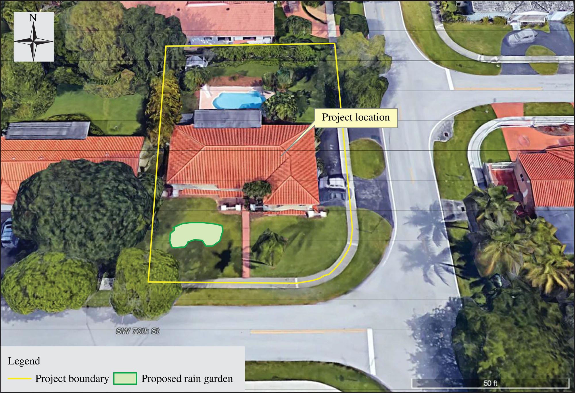
9.7 Rain Garden Design
Similar to GRs, rain gardens provide the similar beneficial effects such as reducing peak flow to sewer system, retaining and degrading nutrients. Example 9.9 presents a design procedure of rain gardens.
Table 9.30 Rain garden depth. Figure 9.10 Project location. Table 9.31 Size factor area. Stormwater treatment technologies managing runoff during rain events are primarily designed to reduce flood risks, settle suspended solids, and concurrently immobilize metals and nutrients. The US EPA TRACI 2.0 (Bare, 2011) can be used to conduct the LCA of the designed rain garden to evaluate the environmental, economic, and social performance of GI stormwater control measures (SCMs). The LCA modeling quantified the environmental impacts associated with the materials, construction, transport, operation, and maintenance of different stormwater management systems. For example, the US EPA TRACI 2.1 lists the eutrophication potential of air and water pollutants (Table 9.32). Table 9.32 The eutrophication potential of air and water pollutants listed by the US EPA TRACI 2.1. The metrics to evaluate benefits and impacts include carbon footprint (global warming potential) in terms of GHG emission, energy utilization, and water withdrawal during the production of the material or systems. The results of this rain garden show that the construction phase is the main contributing life cycle phase for all adverse environmental impacts with total life cycle cost and labor impacts. An EIO‐LCA can be used for the material refining, extraction, production, processing, manufacturing, and transportation phases for the aluminum downspout and gardening plants. The model assesses the impacts of $1 million expenditure on material. As the EIO‐LCA model is linear, the results obtained from the simulation can be scaled to the cost of the materials of the rain gardening system and used to evaluate the impact. The impact of the aluminum downspout used in the project was accessed for the sectors of the economy via EIO‐LCA modeling, and the results of the EIO‐LCA modeling for the GHG emission, energy utilization, and water withdrawal sectors are shown in Tables 9.33, 9.34, 9.35, 9.36, and 9.37, respectively. Although the absolute values could be an good estimate, the relative change of the impacts under different design alternatives could be very important for sustainable EEIS design. Table 9.33 Water withdrawals. Table 9.34 Energy. Table 9.35 Greenhouse gases. Table 9.36 Greenhouse gases. Table 9.37 Energy from all sectors. Rain gardens reduce the overall quantity of runoff by temporarily storing rainwater in a landscaped area before letting it infiltrate the ground. Plants and soils filter out pollutants from the water before returning them to the ground, where they restore groundwater supplies. Rain gardens often result in cost savings by reducing the size of sewer infrastructure. The use of rain gardens may also reduce irrigation costs. Unlike grass or nonnative plants, the native plants used in rain gardens require little water after they are established. Therefore, rain gardens can be designed to meet the necessary runoff volume reduction goal in a cost‐effective way.
Water pollution could be quantified as blue, green, and gray water footprint. The blue water footprint refers to the consumption of blue water resources, such as surface and groundwater, along with the supply chain of a product. Loss of water from the available ground–surface water body in a catchment area is consumed when water evaporates, returns to another catchment area or the sea, or is incorporated into a product. The green water footprint denotes the consumption of green water resources such as rainwater, which is not wasted as runoff. The gray water footprint refers to the volume of freshwater to dilute pollutant concentration to its natural background (Hoekstra et al., 2011). In terms of reducing water footprint rain harvest is the most effective way to reduce green water footprint while gray water reuse is the most effective way to reduce gray water footprint. One of the most widespread, costly, and challenging environmental problems in America is nutrient pollution. Nutrient pollution is caused by excess nitrogen and phosphorus in the air and water. Immense quantities of pollution enter almost all streams without ever flowing through pipes, sewers, treatment plants, or stormwater outfall structures. Such wastewater sources have been characterized as nonpoint source pollution. Nonpoint sources include agricultural areas, abandoned and active mine sites, urban areas and highway facilities, suburban
lawns, and natural areas. It occurs when precipitation falls on the urban environment and picks up pollutants and deposits them into surface waters or introduces them into groundwater. Nitrates and phosphates are nutrients that plants need to grow. In small amounts they are beneficial to many ecosystems. In excessive amounts, however, nutrients cause eutrophication. Eutrophication is the enrichment of an aquatic ecosystem with nutrients that accelerate biological productivity, such as growth of algae and weeds, and an undesirable accumulation of algal biomass. This explosive growth of algae reduces the oxygen in surface water during massive algae die‐off. As a result, estuarine waters could have poor oxygen (hypoxia) or could be completely without oxygen (anoxia). Therefore, prevention using GI such as green roof, rain harvest, rain garden, bioswales, and constructed wetlands is the BMP to combat nonpoint pollution of natural water body and ecosystem.
Slope (%)
Rain garden depth (in)
4
3–5
5–7
6–7
8–12
8
Soil type
3–5 in deep
6–7 in deep
8 in deep
Sandy
0.19
0.15
0.08
Silty
0.34
0.25
0.16
Clayey
0.43
0.32
0.20
9.7.1 Life Cycle Assessment
Substance name
Eutrophication air (kg N eq/kg substance)
Eutrophication water (kg N eq/kg substance)
Phosphorus
1.120
7.290
Phosphorus pentoxide
0.490
3.190
Phosphate
0.366
2.380
Phosphoric acid
0.355
2.310
Nitrogen
0.150
0.986
Ammonium
0.119
0.779
Ammonia
0.119
0.779
Nitric oxide
0.069
0.451
Nitrogen dioxide
0.044
0.291
Nitrogen oxides
0.044
0.291
Nitrate
0.036
0.237
Nitric acid
0.034
0.227
Biological oxygen demand
0.000
0.050
Chemical oxygen demand
0.000
0.050
9.7.2 Environmental Impacts of Aluminum
Sector
Water withdrawals (kgal)
Total of all sectors
19 200.0
221100
Power generation and supply
16 000.0
331314
Secondary smelting and alloying of aluminum
1 410.0
1111B0
Grain farming
356.0
2122A0
Gold, silver, and other metal ore mining
220.0
322130
Paperboard mills
173.0
325510
Paint and coating manufacturing
168.0
33131B
Aluminum product manufacturing from purchased aluminum
142.0
212230
Copper, nickel, lead, and zinc mining
71.0
325190
Other basic organic chemical manufacturing
58.1
325188
All other basic inorganic chemical manufacturing
54.5
Sector
Total energy (TJ)
Coal (TJ)
NatGas (TJ)
Petrol (TJ)
Bio/waste (TJ)
NonFossElec (TJ)
Total of all sectors
24.300
5.390
9.330
1.840
1.700
6.020
33131A
Alumina refining and primary aluminum production
7.210
0.000
1.920
0.061
0.180
5.050
221100
Power generation and supply
6.860
5.000
1.460
0.243
0.000
0.160
33131B
Aluminum product manufacturing from purchased aluminum
5.250
0.000
4.090
0.123
1.040
0.000
331314
Secondary smelting and alloying of aluminum
0.885
0.000
0.586
0.018
0.118
0.163
484000
Truck transportation
0.419
0.000
0.000
0.415
0.000
0.004
331110
Iron and steel mills
0.415
0.246
0.113
0.004
0.002
0.050
322130
Paperboard mills
0.220
0.020
0.015
0.009
0.130
0.015
211000
Oil and gas extraction
0.211
0.000
0.172
0.018
0.000
0.021
324110
Petroleum refineries
0.204
0.000
0.054
0.132
0.010
0.007
325190
Other basic organic chemical manufacturing
0.193
0.024
0.073
0.027
0.058
0.010
Sector
Total t CO2e
CO2 fossil t CO2e
CO2 process t CO2e
CH4 t CO2e
N2O t CO2e
HFC/PFCs t CO2e
Total for all sectors
1560.000
1080.000
195.000
69.700
7.040
206.000
221100
Power generation and supply
563.000
554.000
0.000
1.520
3.440
3.570
33131A
Alumina refining and primary aluminum production
448.000
102.000
159.000
0.000
0.000
187.000
33131B
Aluminum product manufacturing from purchased aluminum
215.000
315.000
0.000
0.000
0.000
0.000
331110
Iron and steel mills
35.800
13.500
22.000
0.218
0.000
0.000
211000
Oil and gas extraction
35.200
9.920
6.450
18.800
0.000
0.000
331314
Secondary smelting and alloying of aluminum
30.900
30.900
0.000
0.000
0.000
0.000
484000
Truck transportation
30.900
30.900
0.000
0.000
0.000
0.000
212100
Coal mining
29.000
3.270
0.000
25.700
0.000
0.000
486000
Pipeline transportation
14.100
6.460
0.018
7.640
0.000
0.000
482000
Rail transportation
13.000
13.000
0.000
0.000
0.000
0.000
Sector
Total t CO2e
CO2 fossil t CO2e
CO2 process t CO2e
CH4 t CO2e
N2O t CO2e
HFC/PFCs t CO2e
Total for all sectors
971.000
649.000
45.100
75.000
199.000
3.100
111400
Greenhouse and nursery production
453.000
307.000
0.000
0.000
146.000
0.000
221100
Power generation and supply
183.000
180.000
0.000
0.495
1.120
1.160
325310
Fertilizer manufacturing
76.800
19.000
25.700
0.000
32.000
0.000
211000
Oil and gas extraction
74.300
20.900
13.600
39.700
0.000
0.000
324110
Petroleum refineries
51.700
51.500
0.000
0.160
0.000
0.000
1121A0
Cattle ranching and farming
14.800
0.972
0.000
8.440
5.430
0.000
484000
Truck transportation
12.800
12.800
0.000
0.000
0.000
0.000
486000
Pipeline transportation
12.600
5.780
0.016
6.850
0.000
0.000
1111B0
Grain farming
9.400
1.390
0.000
0.768
7.250
0.000
221200
Natural gas distribution
6.340
0.573
0.000
5.770
0.000
0.000
Sector
Total energy (TJ)
Coal (TJ)
NatGas (TJ)
Petrol (TJ)
Bio/waste (TJ)
NonFossElec (TJ)
Total of all sectors
11.600
1.720
4.270
4.010
0.159
1.470
111400
Greenhouse and nursery production
6.140
0.000
2.390
2.710
0.000
1.040
221100
Power generation and supply
2.230
1.620
0.475
0.079
0.000
0.052
324110
Petroleum refineries
0.866
0.000
0.231
0.561
0.043
0.031
211000
Oil and gas extraction
0.445
0.000
0.363
0.038
0.000
0.044
325310
Fertilizer manufacturing
0.407
0.002
0.364
0.009
0.005
0.027
484000
Truck transportation
0.174
0.000
0.000
0.172
0.000
0.002
486000
Pipeline transportation
0.151
0.000
0.115
0.000
0.000
0.036
325190
Other basic organic chemical manufacturing
0.144
0.018
0.055
0.020
0.043
0.008
331110
Iron and steel mills
0.062
0.037
0.017
0.000
0.000
0.007
325211
Plastic material and resin manufacturing
0.057
0.002
0.030
0.012
0.006
0.006
9.7.3 Cost and Benefit Analysis of Rain Garden
9.7.4 Water Footprint
9.7.5 Nitrogen and Phosphorus Footprint
9.8 Exercise
9.8.1 Questions
- What are the major design rules in prevention?
- What are the benefits of GI?
- What are the major elements of GI?
- Why is rain harvest so important for a sustainable community?
- What are the different methods in sizing rain harvest tank size?
- In your opinion, what is the order of GI in terms of benefit/cost ratio?
9.8.2 Calculations
- In Miami‐Dade, the annual average precipitation is 60 in. If 80% of the rain can be harvested, answer the following:
- How much water can be harvested for 1 in of rain over a 2000‐ft2 roof?
- What size of the rain harvest tank should be used using three different design methods?
- How much annual saving could be recognized if the irrigation area is 5000 ft2?
- What would be the annual improvement of gray water footprint if the average runoff has 2‐mg/l N and 0.26‐mg/l P due to the rain harvest system for a single‐family house with a 2000‐ft2 roof in Miami‐Dade County if the N and P natural standards are 0.2 and 0.01 mg/l, respectively? What would be the total annual gray water footprint saved if all the single‐family houses of 200 000 installed such rain harvest system in Miami‐Dade County?
9.8.3 Projects
9.8.3.1 Xiongan Project
- Xiongan special economic zone plans to apply GI to maintain clean stormwater discharge to its receiving water body. It has ambitious target to maintain 70% green space and to achieve zero water design. One of the ambitious plans is to require vertical forest house where each apartment should have sufficient large area for trees and grass to combat the smog and water pollution. Collect literature data, and estimate the area required for an apartment of five people to maintain zero water through using gray water for irrigation and rainwater for cooking, shower, and laundry purposes.
- For vertical forest high‐rise building, the challenges are to maximize precipitation areas for rain harvest. However, the high density of the apartment requires different layers of balcony with different arrangement so that each apartment could receive sufficient water for water demand by trees and grass of the balcony. For these reasons, it is critical to team with architectural, structural, and urban planning engineers to achieve zero water design. Form a team with these experts to design a 40‐floor modern residential condo of 800 residences with 4 units on each floor and four people in one apartment.
- From a related website, collect monthly precipitation data in Xiongan, and design the following GI for a sustainable Xiongan:
- Rain harvest system for individual houses.
- GR for high‐rise buildings taller than 40 floors.
- Constructed wetlands throughout the city.
- Use the US EPA software package TRACI 2.0 to conduct the LCA of your design alternatives.
- Compare the corresponding impacts for each alternative, and select the best alternative with supporting quantitative impacts of different categories.
- State your reasons for your selected alternative.
9.8.3.2 Community Proposal Project
- Work with a department of public works or community development, and get an inventory of stormwater management infrastructure in your city.
- Conduct a review, and develop a summary of current literature related to the stormwater benefits of different GIs.
- Identify opportunities to design and build different GIs such as rain harvest, rain gardens, GR, wetland, and on‐site WWT for wherever is appropriate.
- Develop design alternatives of your GI for stormwater management.
- Develop guidelines for the use of rainwater harvesting for stormwater management.
- Conduct cost and benefit analysis of your design alternatives.
- Use the US EPA software package TRACI 2.0 to conduct the LCA of your design alternatives.
- Compare the corresponding impacts for each alternative, and select the best alternative with supporting quantitative impacts of different categories.
- State your reason for your selected alternative.
- Plan and execute the comprehensive GI plan for the community to reduce infiltration/inflow to sewer system by 50%.
References
- Bare, J.C. (2011). TRACI 2.0 – The Tool for the Reduction and Assessment of Chemical and other environmental Impacts. Clean Technologies and Environmental Policies 13 (5): 687–696.
- Center for Neighborhood Technology and American Rivers (2010). The value of green infrastructure: a guide to recognizing its economic, environmental and social benefits. https://www.americanrivers.org/conservation‐resource/value‐green‐infrastructure/ (accessed 22 January, 2018).
- China General Office of the State Council (CGOSC) (2017). Guideline to promote building sponge cities. http://www.gov.cn/zhengce/content/2015‐10/16/content_10228.htm (accessed 16 September 2017).
- Department of Environmental Protection of New York State (DEPNY) (2015). Guidelines for the design and construction of stormwater management systems. Albany: Department of Environmental Conservation.
- EPA (2014). Green infrastructure cost‐benefit resources. http://water.epa.gov/infrastructure/greeninfrastructure/gi_costbenefits.cfm (accessed 12 January 2018).
- Hoekstra, A.Y., Chapagain, A., Martinez‐Aldaya, M., and Mekonnen, M. (2011). The Water Footprint Assessment Manual: Setting the Global Standard. London: Earthscan.
- Jacob, J.S. and Lopez, R. (2009). Is denser greener? An evaluation of higher density development as an urban stormwater‐quality best management practice. Journal of the American Water Resources Association 45 (3): 687–701.
- Lehmann, S. (2010). The Principles of Green Urbanism. UNESCO Chair in Sustainable Urban Development. London: Earthscan.
- Li, H., Ding, L.Q., Ren, M.L. et al. (2017). Sponge City Construction in China: a survey of the challenges and opportunities. Water 9: 594.
- National Bureau of Statistics of China (NBSA) (2015). China Statistical Yearbook 2015. Beijing: China Statistics Press.
- NRC (National Research Council) and NAP (National Academies Press) (2008). Urban Stormwater Management in the United States. Washington, DC: National Academies Press.
- National Research Council (2008). Minerals, Critical Minerals, and the U.S. Economy. Washington, DC: The National Academies Press. https:/doi.org/10.17226/12034 (accessed 19 December 2017).
- Paul, M.J. and Meyer, J.L. (2001). Streams in the urban landscape. Annual Review of Ecology and Systematics 32: 333–365.
- Roy, A., Wenger, S., Fletcher, T. et al. (2008). Impediments and solutions to sustainable, watershed‐scale urban stormwater management: lessons from Australia and the United States. Environmental Management 42 (2): 344–359.
- Sharma, A.K., Pezzaniti, D., Myers, B. et al. (2016). Water Sensitive Urban Design: an investigation of current systems, implementation drivers, community perceptions and potential to supplement urban water services. Water 8: 272.
- United States Environmental Protection Agency (US EPA) (1999). Low‐impact development design strategies: an integrated design approach. EPA 841‐B‐00003. Washington, DC: US EPA.
- The U.S. Green Building Council (USGBC) (2018). Leadership in Energy and Environmental Design (LEED). https://www.usgbc.org/education‐at‐usgbc (accessed January 2018).